Abstract

We analyze a two dimensional SU(3) gauge model of Wilson lines as a dimensionally reduced model of high temperature $QCD_{3}$. In contrast to perturbative dimensional reduction it has an explicit global $Z_{3}$ symmetry in the action. The phase diagram of the model is studied in the space of two free parameters used to describe the self interaction of the Wilson lines. In addition to the confinement-deconfinement transition, the model also exhibits a new $Z_{3}$-breaking phase. These findings are obtained by numerical simulations, and supported by a perturbative calculation to one loop. A screening mass from Polyakov loop correlations is calculated numerically. It matches the known $QCD_{3}$ mass in a domain of parameters belonging to the normal deconfined phase.

^apbialas@th.if.uj.edu.pl
^bmorel@spht.saclay.cea.fr
^cbengt@physik.uni-bielefeld.de

1 Introduction

It would be of considerable interest to understand the long distance properties in the quark gluon plasma quantitatively. Direct simulations of QCD are still too costly to be continued to the continuum limit, at least as far as these properties are concerned. Dimensional reduction has been shown to be a reliable approximation, if the temperature is high enough. In this approach, the non static modes of the fields are integrated out perturbatively, in practice usually to one or two loop order. The resulting effective theory of the static mode is a bosonic field theory in one dimension less [1]–[5]. This becomes a very powerful technique, when the long distance properties are calculated non perturbatively on the lattice in the much simpler reduced theory [6]–[16]. In general one finds that if the temperature is larger than about twice $T_{c}$, the agreement with the full theory in pure gauge theories, where it can be checked, is good. A review of the situation can be found in [17].

In a series of articles [16, 18, 19] we have investigated the dimensional reduction of SU(3) gauge theory in three dimensions to a two dimensional Higgs-gauge-model. In this case one can also easily simulate the full theory and compare the results in detail. We found that using the one loop approximation in the perturbative integration of the non static modes, the reduced model describes very well the correlations between Polyakov loops as well as spacelike Wilson loops down to about $1.5$ times the critical temperature. It should be emphazised that no free parameters are involved, because the lowest order terms of the self-interaction (potential) of the Higgs field are determined by the perturbative calculation.

However, this reduced model does not have the $Z_{3}$ symmetry of the full model. It therefore does not have the confinement-deconfinement phase transition. As we pointed out in [20] one may construct a model, which has the perturbatively reduced model as the high temperature limit, but which does not break the $Z_{3}$ symmetry. Similar models have been discussed in [21, 22].

In this paper we investigate a model where the basic degrees of freedom are the spatial components of the gauge field and the Wilson lines of the three dimensional pure gauge theory. The traces of the latter are the Polyakov loops, order parameters for the preserved $Z_{3}$-symmetry. The Polyakov loop potential is left undetermined and we parametrize it by the first two terms of a small loop expansion. We study the phase diagram of this model in the corresponding parameter plane and show that in addition to the expected confined and deconfined phases, another $Z_{3}$-breaking phase, distinct from the normal deconfined phase, appears.

The Polyakov loops correlation length is also calculated at high temperature along the line corresponding to a purely quadratic potential. It matches that of the original 3D gauge theory at a point which lies inside the normal deconfined phase, not the new one. In this region of parameters, it is thus consistent to view the model as a dimensionally reduced model for $QCD_{3}$, although an effective gain in computing cost requires an a priori knowledge of the Polyakov loops potential, not calculated in this paper.

These calculations are performed via Monte Carlo simulations. First accounts of the numerical results have been presented in [23, 24]. Furthermore we show analytically that the one loop approximation gives a qualitative description of the phase diagram. Although our numerical simulations are restricted to the two dimensional reduced model, the one loop approximation can also be directly applied to the three dimensional case, which is the reduced model of the physical four dimensional QCD. We see in this approximation the same qualitative behaviour of the reduced model, as in the two dimensional case, including the existence of the new phase.

In section 2 we define the reduced model, in section 3 we describe the numerical simulations, and in section 4 we give the corresponding results. In section 5 we derive the effective action of the reduced model in the one loop approximation, and compare with the results of the simulations. We also present the analytic result in the corresponding three dimensional reduced model. Finally section 6 contains a summary of our results.

2 The Model and its Relationship to Finite Temperature $QCD_{3}$

In this section, we first write down the action of the 2D-model under study and then discuss under which conditions it can be viewed as a dimensionally reduced action for the Polyakov loops of pure QCD in 3 dimensions.

The model is defined by its partition function on a square $L^{2}$ lattice with sites ${{\bf x}}$, spanned by unit vectors $\widehat{i}$, i=1,2. The spacing $a$ will be usually set to 1, unless necessary when dimensionful quantities are defined. All dynamical variables belongs to the SU(3) group, gauge fields $U({{\bf x}},i)$ sitting on the links, and matter fields $V({{\bf x}})$, localized on the sites. The variables $V({{\bf x}})$ will be later identified with the Wilson lines of $QCD_{3}$, whose normalized traces are the Polyakov loops. The partition function is written

$$Z = \int{\cal D}U\,{\cal D}V\;\exp{(-S_{U}-S_{U,V}-S_{V})},$$ (1)

$$S_{U} = \beta_{2}\sum_{{{\bf x}}}\,\biggl{(}1-\frac{1}{3}\Re\,\operatorname{Tr}[U({{\bf x}};1)U({{\bf x}}+\widehat{1};2)U^{\dagger}({{\bf x}}+\widehat{2};1)U^{\dagger}({{\bf x}};2)]\biggr{)},$$ (2)

$$S_{U,V} = t\,\sum_{{{\bf x}}}\sum_{i=1,2}\biggl{(}1-\frac{1}{3}\Re\,\operatorname{Tr}[U({{\bf x}};i)V({{\bf x}}+\widehat{i})U^{\dagger}({{\bf x}};i)V^{\dagger}({{\bf x}})]\biggr{)}.$$ (3)

The measure ${\cal D}U\,{\cal D}V$ represents the products of the Haar measures associated with the $U$ and $V$ variables, $S_{U}$ is the 2D Wilson action and $S_{U,V}$ a gauge invariant kinetic term for the matter fields, defining lattice couplings $\beta_{2}$ and $t$. The self-interaction $S_{V}$ is assumed to be a real and locally gauge invariant function of $V$, to be specified later.

Actions of the above type have already been considered in [20, 21, 22] as representative of what an effective action for the Wilson lines of $QCD_{3}$ might look like. A first account of some of our results has been presented in [23, 24].

The connection of the partition function (1) to $QCD_{3}$ may be thought of as follows. Adding a third dimension (a time direction 0), of length $a\,L_{0}$, to the previous lattice, $QCD_{3}$ at temperature $T=1/(a\,L_{0})$ is defined by the 3-dimensional Wilson action on this new lattice and a coupling $\beta_{3}$:

$$S_{QCD_{3}} = \beta_{3}\sum_{x_{0}=1}^{L_{0}}\,\sum_{{{\bf x}}}\,\sum_{\mu<\nu=0}^{2}$$ (4)

$$\biggl{(}1-\frac{1}{3}\Re\,\operatorname{Tr}\,U(x;\mu)\,U(x+\widehat{\mu};\nu)\,U(x+\widehat{\nu};\mu)^{\dagger}\,U(x;\nu)^{\dagger}\biggr{)}.$$

The continuum limit is the limit $a\to 0$ when

$$g_{3}^{2}=\frac{6}{a\,\beta_{3}},$$ (5)

which sets the energy scale, is kept fixed. So we define a dimensionless temperature by

$$\frac{T}{g_{3}^{2}}=\frac{\beta_{3}}{6\,L_{0}},$$ (6)

and fixing the temperature amounts to letting $\beta_{3}$ and $L_{0}$ go to $\infty$ in a fixed ratio. Of course at the same time, the spatial lattice size $a\,L$ is supposed to be large compared to any correlation length. Dimensional reduction [1, 2] provides a way to extract properties of $QCD$ in the large $T/g_{3}^{2}$ regime. The application of the general procedure [3, 4, 5] to $QCD_{3}$ is described in details in [16].

Here we only recall the main steps of the process. In the Wilson action (4), the dynamical field variables $U(x;\mu)\in SU(3)$ are related to the gauge fields by

$$U(x;\mu)\equiv\exp[i\,A_{\mu}(x)].$$ (7)

To make the reduction, we choose a static gauge

$$A_{0}(x_{0},{{\bf x}})=A_{0}({{\bf x}}),$$ (8)

which means

$$U(x_{0},{{\bf x}};0)=U({{\bf x}};0)$$ (9)

for all $x_{0}$. The variables $V({{\bf x}})$, which we call Wilson lines, are defined in this gauge by

$$V({{\bf x}})=U^{L_{0}}({{\bf x}};0)=\exp[i\,L_{0}\,A_{0}({{\bf x}})],\\$$ (10)

and are static operators. Their normalized traces are the gauge invariant Polyakov loops, denoted $v({{\bf x}})$:

$$v({{\bf x}})=\frac{1}{3}\operatorname{Tr}\,V({{\bf x}}).$$ (11)

The spacelike fields $A_{i}(x_{0},{{\bf x}})$, $i=1,2\,,$ can be split into static and non-static components in this gauge,

$$A_{i}^{s}({{\bf x}}) \equiv \frac{1}{L_{0}}\sum_{x_{0}}A_{i}(x_{0},{{\bf x}}),$$ (12)

$$A_{i}^{ns}(x_{0},{{\bf x}}) \equiv A_{i}(x_{0},{{\bf x}})-A_{i}^{s}({{\bf x}}).$$ (13)

The last step of standard dimensional reduction consists in integrating perturbatively over the $A_{i}^{ns}$ fields. For this purpose, the lattice action (4) is expanded to an appropriate order in powers of $A_{0}$ and $A_{i}$, and full gauge fixing is achieved [25, 26] by setting the condition

$$\frac{1}{L_{0}}\,\sum_{x_{0}}\sum_{i=1,2}\,\biggl{(}A_{i}(x_{0},{{\bf x}})-A_{i}(x_{0},{{\bf x}}-\widehat{i})\biggr{)}=0.$$ (14)

Together with Eqs. (12,13), it implies

$$\sum_{i=1,2}\,\biggl{(}A_{i}^{s}({{\bf x}})-A_{i}^{s}({{\bf x}}-\widehat{i})\biggr{)}=0,$$ (15)

which is a lattice Landau gauge for the 2D gauge fields $A_{i}^{s}({{\bf x}})$. By integrating perturbatively over the gauge fields $A_{i}^{ns}(x_{0},{{\bf x}})$ up to one loop order, one gets a two dimensional effective gauge theory of the static modes, where $A_{i}^{s}({{\bf x}})$, $i=1,2\,,$ are the gauge fields and $A_{0}({{\bf x}})$ acts like a Higgs field in the adjoint representation. There are no infrared divergences in this perturbative calculation, and one obtains at a given order in $g_{3}^{2}/T$ only a finite number of interaction terms. The effective two dimensional model has, however, severe infrared divergences in perturbation theory and thus has to be treated non perturbatively. The lattice version of the reduced action is

$$S_{2L}=S_{U}+S_{U,A_{0}}+S_{A_{0}},$$ (16)

$$S_{U}=\beta_{3}L_{0}\sum_{{\bf x}}\biggl{(}1-\frac{1}{3}\Re\,\operatorname{Tr}U({{\bf x}};1)U({{\bf x}}+\widehat{1};2)U^{\dagger}({{\bf x}}+\widehat{2};1)U^{\dagger}({{\bf x}};2)\biggr{)},$$

$$S_{U,A_{0}}=\frac{\beta_{3}L_{0}}{6}\sum_{{{\bf x}}}\sum_{i=1}^{2}\operatorname{Tr}\biggl{(}D_{i}(U)A_{0}({{\bf x}})\biggr{)}^{2},$$ (17)

$$D_{i}(U)A_{0}({{\bf x}})=U({{\bf x}};i)A_{0}({{\bf x}}+\widehat{i})U^{\dagger}({{\bf x}};i)-A_{0}({{\bf x}}),$$

$$S_{A_{0}}=\sum_{{{\bf x}}}k_{2}\,\operatorname{Tr}A_{0}^{2}({{\bf x}})+k_{4}\left(\operatorname{Tr}A_{0}^{2}({{\bf x}})\right)^{2}.$$ (18)

In the above formulae, $S_{U}$ is the pure gauge term in 2D, $S_{U,A_{0}}$ the gauge invariant kinetic term for the scalar Higgs field and $S_{A_{0}}$ the scalar potential, whose self couplings $k_{2}$ and $k_{4}$ result from the one loop integration over the non-static components of the gauge fields [16]. All terms have a global $R_{\tau}$ symmetry $A_{0}({{\bf x}})\,\to\,-A_{0}({{\bf x}})$, while the $Z_{3}$ symmetry of the original 2+1 dimensional SU(3) is broken by the perturbative reduction procedure.

As shown in [16], the 2D model defined by the lattice action (16) successfully accounts for non-perturbative properties of $QCD_{3}$, at $T>1.5\,T_{c}$ and large distances, a conclusion reached from the behaviour of Polyakov loops correlators.

We now examine under which conditions the model of Eq.(1) may also be related to this perturbatively reduced model. First the pure gauge piece $S_{U}$ of Eq.(2) coincides with that of $S_{2L}$ if

$$\beta_{2}=L_{0}\,\beta_{3}.$$ (19)

Next consider the content of $S_{U,V}$, Eq.(3), for $V$ given by (10) and $A_{0}$ small, the situation in which dimensional reduction is known to be justified. To second order in $A_{0}$, Eq.(3) generates the lattice invariant kinetic term

$$\frac{t\,L_{0}^{2}}{6}\,\sum_{{{\bf x}}}\sum_{i=1,2}\operatorname{Tr}\biggl{[}A_{0}^{2}({{\bf x}})+A_{0}^{2}({{\bf x}}+\widehat{i})-2\,U({{\bf x}};i)A_{0}({{\bf x}}+\widehat{i})U^{\dagger}({{\bf x}};i)A_{0}({{\bf x}})\biggr{]},$$ (20)

which coincides with that given by Eq. (17) provided one chooses

$$t=\beta_{3}/L_{0}.$$ (21)

In other words, the coupling $t$ of the model is proportional to the dimensionless temperature defined by Eq. (6).

We finally come to the last term $S_{V}$ in (1), unspecified yet. Of course one would like to be able to compute it from $QCD_{3}$, as it is the case for the self interaction $S_{A_{0}}$, whose lowest order terms (18) were computed perturbatively in the high $T$ and large distances situation [16]. In the absence of a known scheme to do so, we choose the simple form

$$S_{V}=\sum_{{\bf x}}\,\biggl{(}\lambda_{2}\,|v({{\bf x}})|^{2}+\lambda_{3}\,\Re v^{3}({{\bf x}})\biggr{)},$$ (22)

which fulfills the following requirements. It is real and locally gauge invariant. It is also invariant under the global $Z_{3}$ transformation

$$V({{\bf x}})\, \to z_{n}\,V({{\bf x}}),$$ (23)

$$z_{n} = \exp(2\,i\,\pi\,n/3)\,;\quad n=0,1,2\;mod(3).$$

This in fact true for the full action of our model, and distinguishes it from perturbative dimensional reduction. Being an SU(3) matrix, $V({{\bf x}})$ possesses two (invariant) degrees of freedom only, for example two of its three eigenvalues

$$V_{\alpha}({{\bf x}})\equiv\exp\biggl{[}i\,\theta_{\alpha}({{\bf x}})\biggr{]},$$ (24)

$$\prod_{\alpha=1}^{3}\,V_{\alpha}({{\bf x}})=1,$$ (25)

or equivalently the real and imaginary parts of its normalized trace $v({{\bf x}})$, an order parameter for the $Z_{3}$ symmetry. A self-interaction like (22) opens the possibility of a transition from a symmetric phase, where $\langle v({{\bf x}})\rangle$ vanishes, to a broken phase where it has a finite modulus. From this point of view, we consider (22) as the first terms of an expansion of $S_{V}$ near the phase transition. The attempt made in [20] was to fix $\lambda_{2}$ and $\lambda_{3}$ in such a way that, for $A_{0}$ small, $S_{V}$ matches the two lowest order terms of the expansion (18) of $S_{A_{0}}$.

The use of free parameters in $S_{V}$ makes the model less predictive than perturbative reduction at high temperature. In turn, a parametrization like (22) allows to investigate which non-perturbative effects might be associated with lower temperatures. This is why, in what follows, we focuss on the structure of the phase diagram, which we study numerically in the $\{\lambda_{2},\beta_{3}\}$ plane at $\lambda_{3}=0$, the effect of a third order term in $v$ being discussed at a perturbative level only (section 5).

3 Numerical simulations

The model (1) was studied using conventional lattice QCD Monte-Carlo techniques. Lattices of sizes ranging from $L^{2}=16^{2}$ to $72^{2}$ were studied and the parameter $L_{0}$ (the inverse temperature of the $2+1$ model in lattice units) was always set to $4$. The multi hit metropolis algorithm (with 8 hits) was used for updating both the gauge fields $U({{\bf x}},i)$ and the Wilson lines $V({{\bf x}})$. The dynamics of the two sectors were quite different: While the integrated autocorrelation time for the plaquette operator was negligible (of the order of 10 sweeps), for the Wilson lines it could rise up to 25000 sweeps near the phase transition on a $32^{2}$ lattice. One sweep consisted of one update of all the $U$ fields followed by one update of all the $V$ fields. Typically, runs with 2-4 $10^{6}$ sweeps were performed for the system on a $32^{2}$ lattice around the phase transitions.

The quantities measured concerned the Polyakov loops $v({{\bf x}})$ defined in Eq. (11): their lattice averages

$$\mathcal{L}=\frac{1}{L^{2}}\sum_{\bf x}v({\bf x}),$$ (26)

their two–point on axis correlators

$$P(r)=\frac{1}{L^{2}}\langle\sum_{x_{1}}\sum_{x_{2}}v(x_{1},x_{2})v^{*}(x_{1}+r,x_{2})\rangle$$ (27)

and projected correlators :

$$P_{prj}(r)=\frac{1}{L^{2}}\langle\sum_{x_{1}}\sum_{x_{2}}v(x_{1},x_{2})\sum_{x^{\prime}_{2}}v^{*}(x_{1}+r,x^{\prime}_{2})\rangle.$$ (28)

The traces $\mathcal{L}$ were measured and stored on a per configuration basis, so that their distribution $P(\mathcal{L})$ and the susceptibility

$$\chi=\langle|\mathcal{L}|^{2}\rangle-\langle|\mathcal{L}|\rangle^{2}$$ (29)

could be obtained.

The correlators were fitted with the appropriate formulas (see section 4.2) using correlated fit procedures in order to extract screening masses [27].

All the errors were calculated using a blocked bootstrap method. The data were divided into blocks, the size of which was adjusted so as to make them independent from each other, but at least ten blocks were used. Then a bootstrap sample was drawn from those blocks and the measurements performed on this sample. The procedure was repeated 200 times and the standard deviation of the resulting distribution of measured values taken as an estimate of the error on their average.

4 Results from Numerical Simulations

The numerical simulations gave us evidence for the phase diagram in Fig. 1, as we explain below in 4.1. Further in 4.2, we discuss the behaviour of the correlation length measured in the various phases.

4.1 Phase structure

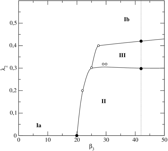
Figure 1: A tentative phase diagram. Open points denote the location of peaks in susceptibility observed on $16^{2}$ lattices. Black points denote the position of phase transitions established on $32^{2}$ lattices with large statistics. The lines are hand drawn sketches of where transitions take place.

We started with simulations of the so-called ‘naive’ model, i.e. with no self-interaction of the Polyakov loops: $S_{V}=0$ in Eq.(1), that is $\lambda_{2}=\lambda_{3}=0$ with the parametrization (22). There the model may also be viewed as standard 2+1 QCD on a lattice with one time slice only. Exploring a range of $\beta_{3}$ values we observed a clear signal for the phase transition expected between a low temperature (low $\beta_{3}$) confined $Z(3)$ symmetric phase (region Ia in Fig. 1) and a broken symmetry high temperature phase (region II).The corresponding peak in the susceptibility occurs at $\beta_{3}$ very close to 20 as shown in Fig. 2, where the average of $|{\cal L}|$ is also shown.

Still keeping $\lambda_{3}=0$, we then performed series of scans in the $\beta_{3}$–$\lambda_{2}$ plane on $16^{2}$ lattices, looking for peaks in the susceptibility (29) as signals for phase transitions and characterizing different phases by the corresponding distributions of $\mathcal{L}$. Although it also includes informations from larger lattices, the tentative phase diagram of Fig. 1 results from this exploration.

\psfrag{L}[.75][0]{$\langle|\mathcal{L}|\rangle$}\includegraphics[width=312.9803pt]{xi.b.eps}

Figure 2: Polyakov loop susceptibility (circles) and average modulus (diamonds) versus $\beta_{3}$ for $\lambda_{2}=\lambda_{3}=0$ on $32^{2}$ lattices. The continuous lines result from Ferrenberg–Swendsen reweighting.

More precise scans in $\lambda_{2}$ along the line $\beta_{3}=42$ ($T\sim 2\,T_{c}$) give for the susceptibility the results plotted in Fig. 3.

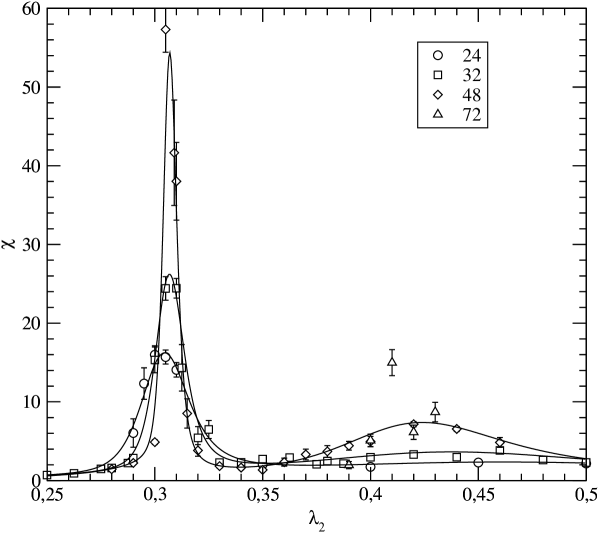
Figure 3: Polyakov loop susceptibility versus $\lambda_{2}$ for $\beta_{3}=42$ and $\lambda_{3}=0$ on lattices of various sizes. The continuous lines result from Ferrenberg–Swendsen reweightings for the three smallest lattices.

A strong transition signal shows up just above $\lambda_{2}=0.3$. There, the time history of $|\mathcal{L}|^{2}$ and the corresponding histogram (Fig. 4) clearly favour a first order phase transition. The height of the peak is furthermore compatible with a $L^{2}$ size dependence in the range $L=24$–$48$, which is the finite size scaling expected for a first order transition.

Figure 4: Time history and histogram for the quantity $|\mathcal{L}|^{2}$, on a $32^{2}$ lattice for $\beta_{3}=42$, $\lambda_{2}=0.305$ and $\lambda_{3}=0$. One clearly sees jumps between two distinct values, and the corresponding double peak structure of the histogram.

The evidence, from similar considerations, for a second phase transition around $\lambda_{2}=0.4$ is considerably weaker. A peak is hardly visible on the same lattices and we had to go to $72^{2}$ lattices (with correspondingly poorer statistics) to ensure that the bump detected does grow with the size. As we will immediately see however, the combination of the above observation with properties of the Polyakov loop distributions confirms the existence of a second transition. Furthermore, the theoretical analysis developed in the next section supports the same conclusion.

In order to identify the nature of the various phases expected from the diagram of Fig. 1, we looked at the corresponding distributions of Polyakov loops. The phases labelled Ia and II are easily identified with standard symmetric and broken $Z(3)$ phases respectively. In Fig. 5, these distributions are shown in the complex plane of $\mathcal{L}$, and they exhibit the expected patterns: The values of $\mathcal{L}$ cluster around 0 in phase Ia, and have a finite modulus and an argument of the form $2\,i\,\pi\,n/3$ in phase II.

As we increase $\lambda_{2}$ from 0 at $\beta_{3}=42$ and move from region II to region III, another symmetry breaking pattern appears. $Z_{3}$ symmetry breaking is again manifested by clusters around non-zero values of $\mathcal{L}$, but now arguments of the form $2\,i\,\pi\,(n+1/2)/3$ are favoured. This is illustrated on Fig. 6 (left). In this example, the lattice is not large enough to prevent the system from tunneling between different phases. Also the run is too short to allow for full equilibration. But accumulations of values of $\mathcal{L}$ close to the boundary with arguments around $\pi$ and $-\pi/3$ are clearly observed. Increasing further $\lambda_{2}$, we move into a region Ib where $Z_{3}$-symmetry is recovered, as shown in Fig. 6 (right). We conjecture that this phase is the same as the low temperature confined phase (Ia).

\psfrag{reL}[.7][0]{$\operatorname{Re}\mathcal{L}$}\psfrag{imL}[.7][0]{$\operatorname{Im}\mathcal{L}$}\includegraphics[width=412.56496pt]{h-I-II-col.eps}

Figure 5: Typical distributions of $\mathcal{L}$ at $\lambda_{2}=\lambda_{3}=0$ for phases Ia ($\beta_{3}=18.0$, left) and II ($\beta_{3}=24$, right).

\psfrag{reL}[.7][0]{$\operatorname{Re}\mathcal{L}$}\psfrag{imL}[.7][0]{$\operatorname{Im}\mathcal{L}$}\includegraphics[width=412.56496pt]{h-III-I-col.eps}

Figure 6: Typical distributions of $\mathcal{L}$ at $\beta_{3}=42$ and $\lambda_{3}=0$ for phases III ($\lambda_{2}=0.32$, left) and Ib ($\lambda_{2}=0.48$, right).

4.2 Screening masses

The inverse of the correlation length between Polyakov loops in the present model corresponds to a screening mass in 2+1 QCD. This screening mass was obtained from the two point Polyakov loop correlators (27) by fitting $m_{S}$ in

$$P(r)\approx a\biggl{(}\frac{e^{-m_{S}r}}{\sqrt{r}}+\frac{e^{-m_{S}(L-r)}}{\sqrt{L-r}}\biggr{)}+c.$$ (30)

The constant $c$ accounts for the fact that we measured unconnected correlators. Fig. 7 provides a comparison of $m_{S}$, as obtained in the present model for $\lambda_{2}=\lambda_{3}=0$ (circles), with previous results (black squares) obtained in the naive perturbative reduction scheme ([16], no Higgs potential). The data are plotted versus the quantity $T/T_{c}\equiv\beta_{3}/\beta_{3c}$, where $\beta_{3c}$ is the critical value of $\beta_{3}$ for $L_{0}=4$, respectively equal to 20 ( this model, see Fig. 1) and to 14.7 in 2+1 QCD [28]. The two sets of points tend to join each other at high temperature. It is the expected result since if $V$ becomes equivalent to an element of $Z_{3}$, it can be rotated to the form (10) with $A_{0}$ small, and the action in (1) can thus be expanded in powers of $A_{0}$. In this situation, if there is no loop potential $S_{V}$ to generate a local Higgs potential, one ends up with the naively reduced model. Near the transition, the two models have very different behaviours. In the perturbative reduction there is no $Z_{3}$ symmetry in the action, correspondingly no phase transition, and the mass does not decrease near the $\beta_{3\,c}$ of the full theory. In the present model, there is a phase transition and the mass decrease from above the transition is consistent with a second order transition. This in accord with the behaviour of $QCD_{3}$.

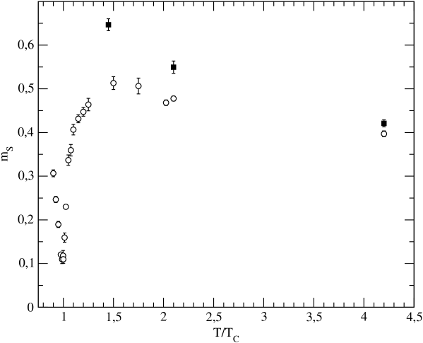
Figure 7: Screening masses in lattice units for the model (1) with $S_{V}=0$ (circles). At large $T$, they approach those obtained in naive dimensional reduction of $QCD_{3}$ (black squares, 2D adjoint Higgs model with no potential [16]).

We also measured the screening masses as a function of $\lambda_{2}$ from our data at $\beta_{3}=42$ and $\lambda_{3}=0$. In this case, we used the projected (0–momentum) correlators (28) and extract the masses by fitting $m_{S}$ in

$$P_{prj}(r)\approx a\bigl{(}e^{-m_{S}r}+e^{-m_{S}(L-r)}\bigr{)}+c.$$ (31)

Our results are summarized in Fig. 8, for three lattice sizes. Important size effects are observed in the region of the ($III\to Ib$) transition just above $\lambda_{2}=0.4$. It is not so near the transition at $\lambda_{2}=0.3$, which is consistent with evidences mentioned earlier which favour a first order transition. It is important to notice that the screening mass at $\beta_{3}$=42 (corresponding to $T/T_{c}\simeq 2$) coincides with the screening mass of $QCD_{3}$ at $\lambda_{2}=0.18$, that is well inside phase II. The situation is different from that in the perturbatively reduced model, where we found the reduction point to be in a metastable $Z_{2}$ symmetric region of parameter space, beyond the transition to the Higgs phase [16, 17].

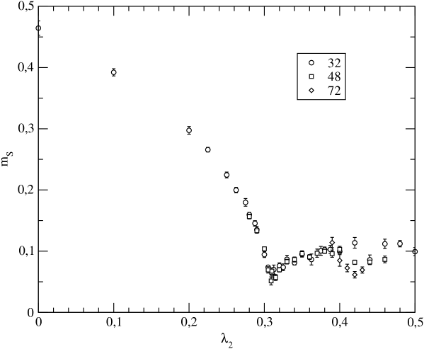
Figure 8: The screening masses $m_{S}$ in lattice units, fitted with Eq. (28) at $\beta_{3}=42$ and $\lambda_{3}=0$, as a function of $\lambda_{2}$ for various lattice sizes.

5 Perturbative Approach to the Polyakov Loops Potential

In order to get further insight into the phase structure of the model, we have performed a perturbative calculation of the effective potential of the Polyakov loops. We assume that in a phase where $Z_{3}$ is spontaneously broken, i.e. where $\langle v({{\bf x}})\rangle$ is not zero, the Wilson line $V({{\bf x}})$ is, up to a local gauge transformation $\Gamma({{\bf x}})$, a constant matrix which we denote $V$. So any local fluctuation of $V({{\bf x}})$ which cannot be gauged away is ignored, and the Polyakov loop $v({{\bf x}})$ is a constant number $v$ on the lattice:

$$V({{\bf x}}) = \Gamma({{\bf x}})\,V\,\Gamma^{\dagger}({{\bf x}}),$$ (32)

$$v({{\bf x}}) = \frac{1}{3}\operatorname{Tr}V({{\bf x}})=\frac{1}{3}\operatorname{Tr}V=v.$$ (33)

Due to gauge invariance of both the action and the measure, $\Gamma({{\bf x}})$ can then be absorbed in a redefinition of the group variables $U$. According to Eqs. (16, 22), the Polyakov loops potential $W_{P}(v)$ defined by

$$\exp\bigl{[}-L^{2}W_{P}(v)\bigr{]}=\int\text{D}[U]\exp\bigl{(}-S\bigr{)},$$

is

$$W_{P}(v)=\lambda_{2}|v|^{2}+\lambda_{3}\Re v^{3}+W(v),$$ (34)

where $W(v)$ is the contribution resulting from the coupling of $V$ to the gauge fields. In order to compute it to one loop order, we first expand $S_{U}+S_{U,V}$ to second order in the SU(3) algebra using

$$U({{\bf x}};i) = \exp[i\,g\,A_{i}({{\bf x}})],$$ (35)

$$A_{i}({{\bf x}}) = \sum_{a=1}^{8}\,T^{a}\,A^{a}_{i}({{\bf x}}),$$

$$\operatorname{Tr}[T^{a}\,T^{b}] = \frac{1}{2}\delta_{ab}.$$

Note that with respect to previous definitions, $A_{i}({{\bf x}})$ has been rescaled by the gauge coupling $g$, where $g^{2}=6/\beta_{2}$. Including the quadratic part of the jacobian from the $U\to\,A$ change of variables, we get

$$S^{(2)}_{A}=\frac{1}{2}\sum_{{{\bf x}}}\Biggl{[}\,\sum_{a=1}^{8}\Biggl{(}A^{a}_{1}({{\bf x}})-A^{a}_{1}({{\bf x}}+\widehat{2})-A^{a}_{2}({{\bf x}})+A^{a}_{2}({{\bf x}}+\widehat{1})\Biggr{)}^{2}$$

$$+\sum_{i=1}^{2}\Biggl{(}\frac{g^{2}\,t}{6}\sum_{a,b=1}^{8}A_{i}^{a}({{\bf x}})A_{i}^{b}({{\bf x}})\biggl{(}2\delta_{ab}-M_{ab}-M_{ba}\biggr{)}+\frac{g^{2}}{4}\sum_{a=1}^{8}\,(A_{i}^{a}({{\bf x}}))^{2}\Biggr{)}\Biggr{]}.$$ (36)

The $8\times 8$ constant matrix $M$ is defined by

$$M_{ab}=2\,\operatorname{Tr}\,[T^{a}\,V\,T^{b}\,V^{\dagger}],$$ (37)

and its properties are derived in the appendix. Since integration over the $A_{i}$’s requires gauge fixing, we then add up to $S^{(2)}_{A}$ the $\xi$-gauge fixing term

$$S_{\xi}=\frac{1}{\xi}\,\sum_{x}\,\sum_{a}\,\biggl{(}A_{1}^{a}({{\bf x}})-A_{1}^{a}({{\bf x}}-\widehat{1})+A_{2}^{a}({{\bf x}})-A_{2}^{a}({{\bf x}}-\widehat{2})\biggr{)}^{2}.$$ (38)

Note that the limit $\xi\to\,0$ reproduces the Landau gauge (15) in which the perturbative reduction was performed. There is no contribution from the ghost terms to the one loop potential. For the rest of the calculation, whose details are given in the appendix, we go to Fourier space, using lattice momentum variables

$$k_{i}=\frac{2\pi n_{i}}{L},\quad\widehat{k}_{i}=2\sin k_{i}/2,\quad\widehat{k}^{2}=\widehat{k}_{1}^{2}+\widehat{k}_{2}^{2}.$$ (39)

The quadratic form in $A_{i}$, diagonal in $k$-space, is a matrix $Q(k)$ in the coordinate$\,\bigotimes\,$colour space so that

$$W(v)=\frac{1}{2\,L^{2}}\,\sum_{k_{1}k_{2}}\log\det Q(k)=\frac{1}{2\,L^{2}}\,\sum_{k_{1}k_{2}}\operatorname{Tr}\log Q(k).$$ (40)

Here, $\operatorname{Tr}$ denotes the trace over both the coordinate and color indices. We obtain

$$Q_{ij}^{ab}=K_{ij}\delta_{ab}-\gamma^{2}\,M_{S,\,ab}\,\delta_{ij},$$ (41)

where

$$\gamma^{2} = \frac{1}{3}\,g^{2}\,t,$$ (42)

$$K_{ij} = (\widehat{k}^{2}+\gamma^{2}+\frac{g^{2}}{4})\,\delta_{ij}-(1-\frac{1}{\xi})\,\widehat{k}_{i}\,\widehat{k}_{j}\,\exp(i\frac{k_{i}-k_{j}}{2}),$$ (43)

$$M_{S} = \frac{1}{2}\,(M+M^{T}).$$ (44)

The diagonalization of $K$ is trivial. That of $M_{S}$ is made in the appendix, where in terms of the eigenvalues (24) of $V$, its eigenvalues $m_{a}$ are shown to be

$$1,\,\,\cos(\theta_{1}-\theta_{2}),\,\,\cos(\theta_{2}-\theta_{3}),\,\,\cos(\theta_{3}-\theta_{1}),$$ (45)

each of them being doubly degenerate. Up to an additive constant in $v$, the one loop contribution to the Polyakov loops effective potential then reads

$$W(v)=\frac{1}{L^{2}}\sum_{k_{1}k_{2}}\,\,\sum_{\alpha<\beta=1}^{3}\,\log\,\biggl{[}\frac{1}{\xi}\,\biggl{(}\widehat{k}^{2}+\frac{g^{2}}{4}+2\,\gamma^{2}\,\sin^{2}\,\frac{\theta_{\alpha}-\theta_{\beta}}{2}\biggr{)}\,\times$$

$$\biggl{(}\widehat{k}^{2}+\xi\,(\frac{g^{2}}{4}+2\,\gamma^{2}\,\sin^{2}\,\frac{\theta_{\alpha}-\theta_{\beta}}{2})\biggr{)}\biggr{]}.$$ (46)

Because the eigenvalues $\exp(i\,\theta_{\alpha})$ of $V$ are not independent, it is more convenient to express $W$ explicitly as a function of the Polyakov loop $v$, which is furthermore an order parameter for the $Z_{3}$ symmetry. This again is performed in the appendix. Specializing to the Landau gauge by taking the limit $\xi\rightarrow 0$ and dropping terms not depending on $v$, we obtain

$$W_{P}(v) = \lambda_{2}|v|^{2}+\lambda_{3}\Re v^{3}+\frac{1}{L^{2}}\sum_{k_{1}k_{2}}\log\,\Biggl{[}\biggl{(}\widehat{k}^{2}+\frac{g^{2}}{4}+\frac{3\gamma^{2}}{2}\biggr{)}^{3}$$ (47)

$$- \frac{9\gamma^{2}}{2}\biggl{(}\widehat{k}^{2}+\frac{g^{2}}{4}+\frac{3\gamma^{2}}{2}\biggr{)}\biggl{(}\widehat{k}^{2}+\frac{g^{2}}{4}+3\,\gamma^{2}\biggr{)}|v|^{2}$$

$$+ \frac{27\gamma^{4}}{2}\biggl{(}\widehat{k}^{2}+\frac{g^{2}}{4}+2\gamma^{2}\biggr{)}\,\Re v^{3}-\frac{81\gamma^{6}}{2^{3}}\,|v|^{4}\Biggr{]}.$$

Using this expression, we studied the shape in $v$ of $W_{P}(v)$ for $\beta_{3}=42$, $L_{0}=4$, $\lambda_{3}=0$ looking for its minimum as a function of $\lambda_{2}$.

For $\lambda_{2}=0$ this minimum is reached at $|v|=1$, i.e. $v=\exp(2i\,n\,\pi/3)$, the standard $Z_{3}$-breaking phase II. Of course the situation remains unchanged for any negative $\lambda_{2}$, which enhances the Boltzmann weight. On the contrary, large $|v|$ values are suppressed for $\lambda_{2}$ positive, and the minimum is at $v=0$ for $\lambda_{2}$ large enough, this is phase Ib. There is however an interval in $\lambda_{2}$ between $\simeq 0.25$ and $0.36$ where the minimum occurs at the non trivial points $v=1/3\,\exp[2\,i\,(n+1/2)\,\pi/3]$, corresponding to the phase III discovered in our numerical simulation inside a similar interval ($\lambda_{2}$ between $\simeq 0.3$ and 0.4, see Fig. 3). The existence of this intermediate phase is due to the cubic term inside the $\log$ of $W(v)$ in Eq. (47), which is minimum for arg$(v^{3})=\pi$.

The situation just described is illustrated in Fig. 9. On the left, we show $W_{P}(v)$ in the complex $v$-plane for $\lambda_{2}=0.32$ inside the phase III, to be compared with the similar plot of Fig. 6 (left), the Boltzmann weight being the largest (resp. smallest) in the blackiest (resp. clearest) regions. On the right, $W_{P}(v)$ is plotted versus $v$ real, for $\lambda_{3}=0$ and three values of $\lambda_{2}$ corresponding to phases II, III, and Ib, as seen from the locations of the minimum, respectively at $v$=1, $v$=–1/3 and $v$=0.

The analysis can be extended to include the effect of the term $\lambda_{3}\Re v^{3}$. From the discussion above, it is clear that a positive (resp. negative) value of $\lambda_{3}$ favours (resp. disfavours) phase III, which is characterized by $\Re v^{3}$ negative. In fact, computing $W_{P}(v)$ for $v$=–1/3, 0, 1 in the $\lambda_{2}$–$\lambda_{3}$ plane, the perturbative phase diagram is easily obtained: At each point the true phase corresponds to the lowest of the three $W_{P}$ values, a (straight) transition line occurs whenever the two lowest coincide, and a triple point when all three are equal. The result is shown in Fig. 10.

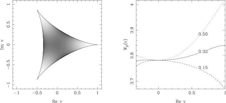
Figure 9: $\beta_{3}=42,\lambda_{3}=0$. On the left, the Polyakov loop potential $W_{P}(v)$ in the $v$-plane at $\lambda_{2}=0.32$. On the right, the shape of $W_{P}(v)$ for $v$ real at three values of $\lambda_{2}$. The positions of the minimum characterize phases II, III, I successively from bottom to top.

Figure 10: The phase diagram in the $\lambda_{2}-\lambda_{3}$ plane, as predicted from the one loop effective potential $W_{P}(V)$ at $\beta_{3}=42$.

The lattice perturbative calculation leading to Eq. (46) is formally similar to that made for SU(2) in Ref. [29]. There, gaussian integration was performed over both the static and non static components of the $QCD_{4}$ spatial gauge fields. As a result of this purely perturbative approach, the $Z_{3}$ symmetry could not be spontaneously broken.

We end up this section with a few remarks.

Remark 1

The perturbative calculation of $W(V)$ can be easily extended to any dimension D. The only change concerns the kinetic part $K_{ij}$ (43) whose indices now run from 1 to D. In the $\xi$-gauge, this K-matrix has $D-1$ eigenvalues equal to $K_{1}$ and one to $K_{2}$, where $K_{1}$ and $K_{2}$ are given by Eq. (63) of the appendix for $\widehat{k}^{2}=\sum_{i=1}^{D}\,\widehat{k}_{i}^{2}$. Then in D-dimensions the perturbative result (47) reads

$$W_{P}(v) = \lambda_{2}|v|^{2}+\lambda_{3}\Re v^{3}+\frac{D-1}{L^{2}}\sum_{k_{1}k_{2}...k_{D}}\log\,\Biggl{[}\biggl{(}\widehat{k}^{2}+\frac{g^{2}}{4}+\frac{3\gamma^{2}}{2}\biggr{)}^{3}$$ (48)

$$- \frac{9\gamma^{2}}{2}\biggl{(}\widehat{k}^{2}+\frac{g^{2}}{4}+\frac{3\gamma^{2}}{2}\biggr{)}\biggl{(}\widehat{k}^{2}+\frac{g^{2}}{4}+3\,\gamma^{2}\biggr{)}|v|^{2}$$

$$+ \frac{27\gamma^{4}}{2}\biggl{(}\widehat{k}^{2}+\frac{g^{2}}{4}+2\gamma^{2}\biggr{)}\,\Re v^{3}-\frac{81\gamma^{6}}{2^{3}}\,|v|^{4}\Biggr{]}.$$

Using it in dimension 3, we find that the phase structure represented in Fig. 10 persists, with similar values of $\lambda_{2}$ and $\lambda_{3}$ on the transition lines if the parameters $\gamma^{2}$ and $g^{2}$ are kept the same.

Remark 2

Heuristic arguments neglecting any entropic consideration help to understand the phase diagram found, including the new phase III. The part $S_{U,V}$ of the action is trivially minimized if the commutator $[U,V]$ vanishes for any $U$, which implies $V\in Z_{3}$, i.e. in phase II. Conversely, typically for $\lambda_{2}>0$ and $\lambda_{3}=0$, $S_{V}$ is minimized by $v$=0 (phase I) and there is a competition. A possible compromise is to require $V$ to commute with all the elements of an SU(2) subgroup of SU(3), that is to be proportional to a $Z_{2}$ subgroup of $Z_{3}$: In diagonal form, $V=$diag$[\exp(i\theta),\,\exp(i\theta),\,\exp(-2i\theta)]$, up to colour index permutations. In this subset $|v|$ is minimum for $\theta=(2\,n+1)\pi/3$, and there $v=1/3\,\exp[i\,(2\,n+1)\pi/3]$ is in phase III.

Remark 3

The physical region for $v$ is limited by the condition that two (or three) eigenvalues of $V$ are equal. The points characterizing phases II and III belong to this boundary, and the measure ${\cal D}\,V$ vanishes there. This contributes a logarithmic repulsive potential on the boundary. Its effect is expected to repell the values of $v$ in phases II and III slightly inside the physical region, and to change the exact position of the transitions lines.

6 Summary

We have investigated a model for Wilson lines coupled to a $SU(3)$ gauge field in two dimensions. This model was inspired by dimensional reduction of three dimensional $SU(3)$ gauge theory. It is a $Z_{3}$ symmetric Higgs model with the Wilson line acting as a Higgs field in the adjoint representation of the group. In perturbative dimensional reduction, where the $Z_{3}$ symmetry is explicitly broken, the self couplings of the corresponding Higgs field are determined by the perturbative integration of the non static modes in the original theory. Here we have left the selfcouplings free parameters, to be eventually determined from the full model. The price paid is a loss in predictive power, but the model allowed us to investigate in detail a non trivial phase diagram, which includes the confinement-deconfinement transition of $QCD_{3}$.

In fact, the model exhibits three different phases. The order parameter is the trace of the Wilson line, i.e. the Polyakov loop. At low values of $\beta_{2}$ we find a confined phase, where the Polyakov loop is distributed around zero. Above a transition we find for $\lambda_{2}=0$ a deconfined phase, where the Polyakov loop is near to an element of $Z_{3}$, one of the third roots of unity. Keeping $\beta_{2}$ fixed in the deconfined phase and letting $\lambda_{2}$ grow we find a first order phase transition into a new phase, where the Polyakov loops are situated near the boundary of phase space but with a phase half way in between the third roots of unity. Here also, $Z_{3}$ symmetry is spontaneously broken, but the Wilson line is near to an element of a $Z_{2}$ subgroup of SU(3). If we increase $\lambda_{2}$ even more we come into a confined phase again.

We also have measured the screening masses from the Polyakov loop correlations. They become small near the deconfinement phase transition. If one uses the screening mass to compare with the full model, in order to find the values of the coupling constants which correspond to dimensional reduction, one finds it to be in the normal deconfined phase.

Considering this Wilson line model as a possible dimensionally reduced model of three dimensional SU(3) gauge theory, and comparing it with usual perturbative dimensional reduction one finds that

- the model has explicit $Z_{3}$ symmetry in the action, in contrast to the perturbatively reduced model, where the symmetry is explicitely broken.

- it has a confinement-deconfinement transition in contrast to the perturbatively reduced model

- at this deconfinement transition, which is in the same universality class as full $QCD_{3}$, the screening masses should go to zero.

- the reduction point in parameter space seems to lie in the physical phase, in contrast to the perturbative reduction, where it is in the metastable region inside the Higgs phase

All these properties makes the Wilson line model an interesting extension of dimensional reduction, if one wants to approach the phase transition, while perturbative reduction can only be used at temperatures higher than about two times the critical temperature.

There are several interesting questions that can be further investigated. In particular one would like to extend the numerical calculation to three dimensions, where one would have a dimensionally reduced model of $(3+1)D$ QCD, i.e. the physical theory. Furthermore one should address the question if the new phase plays any role at high temperature or high temperature and finite density QCD. It is of course also important to restrain the parameters, so as to get quantitative predictions without parameters, as it is the case in perturbative dimensional reduction.

7 Acknowledgments

All the simulations were done on the PC–farm donated to P.B. by the Alexander von Humbold Foundation. In 2003–2004, P.B. was partially supported by the KBN grant 2P03B 083 25. B.P. is grateful to the Service de physique théorique de Saclay (France) for support and kind hospitality. B.P. and P.B. also thank DFG for support under the contract FOR 339/2-1.

Appendix A Calculation of the Perturbative Polyakov Loops Potential

Here we derive the expressions (45) of the eigenvalues of the M-matrix, and the final expression of the potential as a function of the Polyakov loop. The following two trace identities in SU(3) will be used extensively

$$\sum_{a}\,\operatorname{Tr}(T^{a}XT^{a}Y)=\frac{1}{2}\biggl{(}\operatorname{Tr}X\,\operatorname{Tr}Y-\frac{1}{3}\,\operatorname{Tr}(XY)\biggr{)},$$ (49)

$$\sum_{a}\,\operatorname{Tr}(T^{a}X)\,\operatorname{Tr}(T^{a}Y)=\frac{1}{2}\biggl{(}\operatorname{Tr}(XY)-\frac{1}{3}\,\operatorname{Tr}X\,\operatorname{Tr}Y\biggr{)}.$$ (50)

Recalling that $\operatorname{Tr}T^{a}=0$, one first shows from its definition (37) that the matrix $M(V)$ is real and fulfills

$$M^{T}(V) = M(V^{\dagger})$$

$$M(V^{\dagger})\,M(V) = M(V)\,M(V^{\dagger})=I,$$ (51)

$$M^{p}(V) = M(V^{p}).$$ (52)

Hence $M$ is orthogonal. In the matrix $Q$ of Eq. (41), we factorize the matrix $K$ of Eq. (43), call $K_{i}$ its eigenvalues and write

$$\operatorname{Tr}\log Q = \operatorname{Tr}\log K+X,$$

$$\operatorname{Tr}\log K = \log\,K_{1}^{8}\,+\,\log\,K_{2}^{8},$$

$$X = -\sum_{p=1}^{\infty}\,\frac{\gamma^{2p}}{p\,2^{p}}\,\operatorname{Tr}\biggl{(}K^{-p}\,\biggl{[}\,M(V)+M(V^{\dagger})\,\biggr{]}^{p}\biggr{)}.$$ (53)

Note that $K^{-1}$ exists for any $\xi>0$. The Landau gauge is reached in the limit $\xi\to 0$ The trace involved in $X$ is the product of $K_{1}^{-p}+K_{2}^{-p}$ by the trace $m_{p}$ in color space of $(M+M^{\dagger})^{p}$,

$$m_{p}=\sum_{a=1}^{8}\,\biggl{(}\biggl{[}M(V)+M(V^{\dagger})\biggr{]}^{p}\biggr{)}_{aa}.$$ (54)

In this expression, we expand $(M+M^{\dagger})^{p}$ and apply (52):

$$m_{p}=4\,\sum_{q=0}^{p}\,C_{p}^{q}\,\sum_{a,b=1}^{8}\,\operatorname{Tr}\biggl{[}T^{a}\,V^{q}\,T^{b}\,V^{\dagger q}\biggr{]}\,\,\operatorname{Tr}\biggl{[}T^{b}\,V^{\dagger\,p-q}\,T^{a}\,V^{p-q}\biggr{]}.$$ (55)

Repeated use of (49, 50) to sum over color indices leads to

$$m_{p}=\sum_{q=0}^{p}\,C_{p}^{q}\,\biggl{(}\operatorname{Tr}\biggl{[}V^{q}\,V^{\dagger p-q}\biggr{]}\,\,\operatorname{Tr}\biggl{[}V^{\dagger q}\,V^{p-q}\biggr{]}\,-1\biggr{)}.$$ (56)

Let $V_{\alpha}\equiv\exp(i\,\theta_{\alpha})$, $\alpha=1,2,3$ be the eigenvalues of $V$; those of $V^{\dagger}$ are $1/V_{\alpha}$ so that

$$m_{p} = \sum_{q=0}^{p}\,C_{p}^{q}\,\Biggl{(}\sum_{\alpha,\beta=1}^{3}\,\biggl{(}\frac{V_{\alpha}}{V_{\beta}}\biggr{)}^{2q-p}-1\Biggr{)}$$ (57)

$$= 2\,\Biggl{(}2^{p}+\sum_{\alpha<\beta}\biggl{(}\frac{V_{\alpha}}{V_{\beta}}+\frac{V_{\beta}}{V_{\alpha}}\biggr{)}^{p}\Biggl{)}.$$

In Eqs. (53), the resummation over p gives $X$, and $W$ follows. Up to additive constants independent of $V$, $X$ and $W$ are then given by

$$X = 2\,\sum_{i=1}^{2}\,\log\Biggl{[}\,\prod_{\alpha<\beta=1}^{3}\,\Biggl{(}1-\frac{\gamma^{2}}{2\,K_{i}}\,\biggl{(}\frac{V_{\alpha}}{V_{\beta}}+\frac{V_{\beta}}{V_{\alpha}}\biggr{)}\Biggr{)}\Biggr{]},$$ (58)

$$W(V) = \frac{1}{L^{2}}\,\sum_{k_{1}k_{2}}\,\sum_{i=1}^{2}\log\,\Biggl{[}\,\prod_{\alpha<\beta=1}^{3}\,\Biggl{(}K_{i}-\frac{\gamma^{2}}{2}\biggl{(}\frac{V_{\alpha}}{V_{\beta}}+\frac{V_{\beta}}{V_{\alpha}}\biggr{)}\Biggr{)}\Biggr{]}.$$ (59)

Eq. (58) proves that the eigenvalues of the symmetric part of $M$ are $\Re\,V_{\alpha}/V_{\beta}=cos(\theta_{\alpha}-\theta_{\beta})$, as stated in (45). The next task is to express $W$ as a function of $\operatorname{Tr}V$, and for this we have to evaluate the product

$$P=\prod_{\alpha<\beta=1}^{3}\,\biggl{(}1-\tau\,\frac{V_{\alpha}^{2}+V_{\beta}^{2}}{V_{\alpha}\,V_{\beta}}\biggr{)}$$ (60)

for $\tau\equiv\gamma^{2}/(2\,K_{i})$. Set $P=\sum_{n=0}^{3}(-1)^{n}\,c_{n}\,\tau^{n}$ and use $V_{1}\,V_{2}\,V_{3}=1$. We have $c_{0}=1$ and, $c.p.$ denoting the circular permutations of $\{1\,2\,3\}$,

$$c_{1} = (V_{1}^{2}+V_{2}^{2})\,V_{3}\,+\,c.p.$$

$$c_{2} = (V_{1}^{2}+V_{2}^{2})\,V_{3}\,(V_{2}^{2}+V_{3}^{2})\,V_{1}\,+\,c.p.$$

$$c_{3} = (V_{1}^{2}+V_{2}^{2})\,(V_{2}^{2}+V_{3}^{2})\,(V_{3}^{2}+V_{1}^{2}).$$

Replacing systematically $V_{\alpha}^{2}+V_{\beta}^{2}$ by $\operatorname{Tr}V^{2}-V_{\gamma}^{2}$ whenever $\alpha,\beta,\gamma$ are different, we find

$$c_{1} = \operatorname{Tr}V^{2}\,\operatorname{Tr}V\,-\,\operatorname{Tr}V^{3},$$

$$c_{2} = \operatorname{Tr}V^{2}\,\operatorname{Tr}V\,+\,\operatorname{Tr}V^{\dagger\,3},$$ (61)

$$c_{3} = \operatorname{Tr}V^{2}\,\operatorname{Tr}V^{\dagger\,2}\,-\,1.$$

Now $\operatorname{Tr}V^{n}$ for $n>1$ is a polynomial of degree n in $\operatorname{Tr}V$ (for general formulae, see Appendix A in [18]). In particular

$$\operatorname{Tr}V^{2} = (\operatorname{Tr}V)^{2}\,-\,2\,\operatorname{Tr}V^{\dagger},$$

$$\operatorname{Tr}V^{3} = (\operatorname{Tr}V)^{3}\,-\,3\,|\operatorname{Tr}V|^{2}\,+\,3.$$

Substituting these expressions into Eqs.(61) and using $v=1/3\,\operatorname{Tr}\,V$ provide the desired result: Up to an additive constant, the perturbative part of the Polyakov loop potential is

$$W(v)=\frac{1}{L^{2}}\,\sum_{k_{1}k_{2}}\,\sum_{i=1}^{2}\log\Biggl{[}(\frac{\gamma^{2}}{2}+K_{i})^{3}$$

$$-\frac{9\gamma^{2}}{2}(\frac{\gamma^{2}}{2}+K_{i})(2\gamma^{2}+K_{i})|v|^{2}+\frac{27\gamma^{4}}{2}(\gamma^{2}+K_{i})\Re v^{3}-\frac{81\gamma^{6}}{2^{3}}|v|^{4}\Biggr{]},$$ (62)

where the eigenvalues $K_{i}$ are

$$K_{1}=\widehat{k}^{2}+\gamma^{2}+\frac{g^{2}}{4}\quad;\quad K_{2}=\frac{\widehat{k}^{2}}{\xi}\,+\,\gamma^{2}+\frac{g^{2}}{4}$$ (63)

References

- [1] P. Ginsparg, Nucl. Phys. B170 (1980) 388.
- [2] T. Appelquist and R. Pisarski, Phys. Rev. D23 (1981) 2305.
- [3] S. Nadkarni, Phys. Rev. (1983) 917; Phys. Rev. (1988) 3287.
- [4] N. P. Landsman, Nucl. Phys. B322 (1989) 498.
- [5] T. Reisz, Z. f. Phys. (1992) 169.
- [6] P. Lacock, D. E. Miller and T. Reisz, Nucl. Phys. B369 (1992) 501.
- [7] L. Kärkäinen, P. Lacock, D. E. Miller, B. Petersson and T. Reisz, Phys. Lett. B282 (1992) 121.
- [8] L. Kärkäinen, P. Lacock, D. E. Miller, B. Petersson and T. Reisz, Phys. Lett. B282 (1992) 121.
- [9] K. Kajantie, M. Laine, K. Rummukainen and M. Shaposnikov, Nucl. Phys. B503 (1997) 357
- [10] K. Kajantie, M. Laine, A. Rajantie, K. Rummukainen and M. Tsypin, JHEP 9811 (1998) 011
- [11] S. Datta and S.Gupta, Phys. Lett.B471 (2000) 382; Nucl. Phys. B534 (1998) 392
- [12] M. Laine and O. Philipsen, Nucl. Phys. B523 (1998) 291; Phys. Lett. B459 (1999) 259.
- [13] A. Hart and O. Philipsen, Nucl. Phys. B572 (2000) 243.
- [14] A. Hart, M. Laine and O. Philipsen, Nucl. Phys. B586 (2000) 443.
- [15] F. Karsch, M. Oevers and P. Petreczky, Phys. Lett B442 (1998) 291; A. Cucchieri, F. Karsch and P. Petreczky, Phys. Rev. D64 (2001) 036001.
- [16] P. Bialas, A. Morel, B. Petersson, K. Petrov and T. Reisz, Nucl. Phys. B581 (2000) 477.
- [17] O. Philipsen, Nucl. Phys. Proc. Suppl. 94 (2001) 49.
- [18] P. Bialas, A. Morel, B. Petersson, K. Petrov and T. Reisz, Nucl. Phys. B603 (2001) 369
- [19] P. Bialas, A. Morel, B. Petersson and K. Petrov, Nucl. Phys. Proc. Suppl. 106 (2002) 882
- [20] P. Bialas, A. Morel, B. Petersson and K. Petrov, “Z(3) Symmetric Dimensional Reduction of (2+1)D QCD”, Proceedings of the International Symposium on Statistical QCD, [arXiv:hep-lat/0112008].
- [21] T. Banks and A. Ukawa, Nucl. Phys B225 (1983) 145.
- [22] R. D. Pisarski, Phys. Rev. D62 (2000) 111501; Nucl. Phys. A702 (2002) 151; A. Dumitru and R. D. Pisarski, Phys. Rev. D66 (2002) 096003
- [23] P. Bialas, A. Morel and B. Petersson, “Dimensional reduction and a Z(3) symmetric model”, to appear in the Proceedings of the XXI International Symposium on Lattice Field Theory, (Tsukuba, Japan, 2003) [arXiv: hep-lat/0309190].
- [24] P. Bialas, A. Morel and B. Petersson, “Dimensional reduction in QCD: Lessons from lower dimensions”, to appear in the Proceedings of the Workshop on Finite Density QCD at Nara (Nara, 10-12 July, Japan, 2003).
- [25] C. Curci and P. Menotti, Z. f. Phys. C21 (1984) 281; C. Curci, P. Menotti and G. Paffuti, Z. f. Phys. C26 (1985) 549.
- [26] T. Reisz, Jour. Math. Phys. 32 (1991) 515
- [27] C. Michael and A. McKerrell, Phys. Rev. D51 (1995) 3745 [arXiv:hep-lat/9412087].
- [28] C. Legeland, Ph.D. Thesis “Aspects of (2+1) Dimensional Lattice Gauge Theory” (Univ. of Bielefeld, 1998)
- [29] N. Weiss, Phys. Rev. D24 (1981) 475.