An asymptotic formula for the pion decay constant in a large volume

Abstract

We derive an asymptotic formula à la Lüscher for the finite volume correction to the pion decay constant: this is expressed as an integral over the $\langle 3\pi|A_{\mu}|0\rangle$ amplitude after proper subtraction of the pion pole contribution. We analyze the formula numerically at leading and next-to-leading order in the chiral expansion.

1. Introduction

The analytical study of finite volume effects is becoming of increasing importance as lattice calculations with dynamical fermions approach smaller quark masses and aim at higher precision. Since these effects are dominated by the lightest particles in the spectrum, the pions, and by their long distance dynamics, one can study them in the framework of chiral perturbation theory (CHPT) [1]. A number of analyses of these effects in different quantities have recently appeared in the literature [2, 3]. One of these concerned the case of the pion mass [2] and has shown that a leading order calculation may receive very large corrections from the next-to-leading contribution even for small values of the quark masses, whereas even higher order corrections behave according to expectations and show a convergent behaviour. This accurate study of the convergence of the chiral series has been made possible by the use of Lüscher’s asymptotic formula for the pion mass [4]. The formula relates its leading finite-volume corrections to an integral over the $\pi\pi$ scattering amplitude in infinite volume. Since the latter is known to next-to-next-to-leading order in the chiral expansion [5], it is straightforward to evaluate Lüscher’s formula to the same order in the chiral expansion.

In view of the results for the pion mass, the question arises if one can derive similar asymptotic formulae also for other quantities: as we will show in what follows, this is the case. In the present article we concentrate on $F_{\pi}$, derive an asymptotic formula which relates it to the infinite-volume $\langle 3\pi|A_{\mu}|0\rangle$ amplitude and analyze it numerically using the next-to-leading order calculation of this amplitude [6]. The results show again large next-to-leading order corrections – in this case we cannot explore the chiral expansion further because the two-loop calculation of the $\langle 3\pi|A_{\mu}|0\rangle$ amplitude is not yet available.

2. The asymptotic formula

Denote by $F_{\pi,L}$ the pion decay constant in a box of size $L$. The asymptotic formula for $\Delta F_{\pi}=F_{\pi,L}-F_{\pi}$ can then be written as:

$$\Delta F_{\pi}=\frac{3}{8\pi^{2}M_{\pi}L}\int_{-\infty}^{\infty}dy\;e^{-\sqrt{M_{\pi}^{2}+y^{2}}L}N_{F}(iy)+O(e^{-\bar{M}L})\;\;,$$ (1)

where $\bar{M}\!\geq\!\sqrt{3/2}\>M_{\pi}$ and the amplitude $N_{F}(\nu)$ is defined as follows. Consider the amplitude for creation of three pions out of the vacuum with the axial current:

$$\langle\pi^{1}(p_{1})\pi^{1}(p_{2})\pi^{3}(p_{3})|A^{3}_{\mu}(0)|0\rangle = (p_{1}+p_{2})_{\mu}G(s_{1},s_{2},s_{3})$$

$$+ (p_{1}-p_{2})_{\mu}H(s_{1},s_{2},s_{3})+p_{3\,\mu}F(s_{1},s_{2},s_{3})\;\;,$$

where the superscripts on the pion states and axial current are isospin indices and $G$, $H$ and $F$ are three scalar amplitudes of the variables $s_{1}$,$s_{2}$ and $s_{3}$, with $s_{1}=(p_{2}+p_{3})^{2}$ and cyclic permutations [6]. From the amplitude (2. The asymptotic formula) one can construct the combination which has two of the outcoming pions in an $I=0$ state (the explicit relation is given below)

$$\langle(2\pi)_{I=0}\pi^{3}(p_{3})|A^{3}_{\mu}(0)|0\rangle = (p_{1}+p_{2})_{\mu}G_{0}(s_{1},s_{2},s_{3})$$

$$+ (p_{1}-p_{2})_{\mu}H_{0}(s_{1},s_{2},s_{3})+p_{3\,\mu}F_{0}(s_{1},s_{2},s_{3})\;\;.$$

This amplitude contains a pole in the unphysical region, for $(p_{1}+p_{2}+p_{3})^{2}=Q^{2}=M_{\pi}^{2}$, which needs to be removed before proceeding further. We define

$$\langle(2\pi)_{I=0}\pi^{3}(p_{3})|A^{3}_{\mu}(0)|0\rangle_{S} = \langle(2\pi)_{I=0}\pi^{3}(p_{3})|A^{3}_{\mu}(0)|0\rangle$$ (4)

$$- Q_{\mu}\frac{iF_{\pi}T^{I=0}(s_{3},s_{1}-s_{2})}{M_{\pi}^{2}-Q^{2}}\;\;,$$

where $T^{I=0}(s,t-u)$ is the $\pi\pi$ scattering amplitude with isospin zero in the $s$ channel. We need the subtracted amplitude in the forward kinematic configuration, i.e. for $p_{1}=-p_{2}$, $s_{3}=0$, where it becomes a function of one variable only, $\nu=(s_{2}-s_{1})/(4M_{\pi})$:

$$p_{3}^{\mu}\langle(2\pi)_{I=0}\pi^{3}(p_{3})|A^{3}_{\mu}(0)|0\rangle_{S\;|_{p_{1}=-p_{2}}}=2M_{\pi}\nu h_{0}(\nu)+M_{\pi}^{2}\bar{f}_{0}(\nu)\;\;,$$ (5)

where

$$h_{0}(\nu)=H_{0}(2M_{\pi}(M_{\pi}\!-\!\nu),2M_{\pi}(M_{\pi}\!+\!\nu),0)$$

and analogously for $\bar{f}_{0}$ and where the bar on the $F_{0}$ form factor denotes that it is defined after subtraction of the pion pole (the form factor $H_{0}$ remains unaffected by the subtraction). The amplitude $N_{F}$ which enters the asymptotic formula for the finite volume corrections to $F_{\pi}$ is defined as

$$N_{F}(\nu)=-i\left(2\nu h_{0}(\nu)+M_{\pi}\bar{f}_{0}(\nu)\right)\;\;.$$ (6)

The amplitudes $H_{0}$ and $F_{0}$ can be expressed in terms of $F$, $G$ and $H$ appearing in (2. The asymptotic formula):

$$F_{0}(s_{1},s_{2},s_{3}) \!\!=\!\! 3F_{123}+G_{231}+G_{312}-H_{231}+H_{312}\;\;,$$

$$H_{0}(s_{1},s_{2},s_{3}) \!\!=\!\! 3H_{123}+\frac{1}{2}\left[F_{231}-F_{312}-G_{231}+G_{312}-H_{231}-H_{312}\right],\;\;$$ (7)

where $X_{ijk}=X(s_{i},s_{j},s_{k})$ with $X=F,G,H$.

3. Outline of the derivation

The derivation of this formula is in large parts analogous to the derivation of the formula for the pion mass, due to Lüscher [4]. In the following we simply outline the necessary steps to prove the formula and refer the reader to the paper of Lüscher for details. The starting point of the analysis is that one can rely on an effective Lagrangian description of the relevant physics and analyze these finite volume effects in CHPT. As observed by Lüscher, the precise form of the effective Lagrangian is never needed in the proof – on the other hand, it is very useful to have it available if one wants to understand in concrete terms these effects. As was shown by Gasser and Leutwyler one can rigorously derive the consequence of chiral symmetry also if the system is closed inside a large finite volume with the help of the effective Lagrangian technique [1]. In particular the form of the local effective Lagrangian remains unchanged, and the only difference with respect to infinite volume calculations comes from the propagator for the pion field which becomes periodic in all spatial directions

$$G(x^{0},\vec{x})=\sum_{\vec{n}\in\mathbb{Z}^{3}}G_{0}(x^{0},\vec{x}+\vec{n}L)$$ (8)

where $G_{0}(x)$ is the propagator in infinite volume.

The first step in Lüscher’s proof of the asymptotic formula for the pion mass consists in showing that, for a generic loop diagram contributing to the self energy of the pion, the dominating finite volume effect is obtained if one takes all propagators in infinite volume ($G(x)\to G_{0}(x)$) except one, for which only the terms with $|\vec{n}|=1$ in the sum in (8) should be kept. The sum of all possible contributions of this form from all possible loop diagrams gives the leading finite volume corrections to the pion mass. The same conclusion is valid also for the Feynman diagrams which renormalize the coupling between the axial current and the pion – the fact that in this case one of the external legs is the axial current instead of a pion does not touch the argument at all.

Figure 1: Graphical representation of the asymptotic formula. The wiggly (straight) line represents the axial current (pion). The dash on the propagator means that it is taken in finite volume (only the contribution with $|\vec{n}|=1$ in the sum (8)). Diagram a (b) illustrates the correction to $F_{\pi}$ (the shift of the pole position) due to finite volume.

The second step in the proof consists in showing, by modifying the integration contour in the complex plane, that this leading contribution can be written in a very compact form, as an integral over an amplitude (the $\pi\pi$ scattering amplitude in the case of the pion mass) defined in Minkowski space, analytically continued to complex values of its arguments. Again, the same argument applies also to the case of the pion decay constant: in this case, in all possible loop graphs that renormalize the pion coupling to the axial current we have to single out one internal pion propagator, break it up and put the resulting two external legs on shell. The relevant amplitude in this case is the $\langle 3\pi|A_{\mu}|0\rangle$ amplitude, as illustrated in Fig. 1a – the weight function which appears in the integral is however exactly the same as in the pion mass case.

The kinematic configuration in which the amplitude must be evaluated is also the same and corresponds, for the $\pi\pi$ amplitude, to forward scattering. The $\langle 3\pi|A_{\mu}|0\rangle$ amplitude is however singular for this kinematics because of a pole due to one-pion exchange among the axial current and the three outgoing pions. This singularity does not belong to the finite volume corrections to $F_{\pi}$ and should be subtracted. The reason for the presence of this pole can be explained as follows: the $\langle\pi|A_{\mu}|0\rangle$ amplitude is defined as the residue at the pion pole of a two-point function of the axial current and any interpolating field for the pion:

$$\langle\pi^{a}(q)|A^{b}_{\mu}|0\rangle = \lim_{q^{2}\to M_{\pi}^{2}}(M_{\pi}^{2}-q^{2})iq_{\mu}\delta^{ab}P(q)$$ (9)

$$P(q) = N_{\phi}q^{\mu}\int dxe^{iqx}\langle 0|T\phi^{1}_{\pi}(x)A^{1}_{\mu}(0)|0\rangle\;\;,$$

with $N_{\phi}$ the proper normalization factor which depends on the field $\phi_{\pi}$. In finite volume both the residue as well as the position of the pole are shifted. Ignoring the latter shift corresponds to multiplying $P_{L}(q)$ by $(M_{\pi}^{2}-q^{2})$ and not by the correct $(M_{\pi,L}^{2}-q^{2})$ and then taking the limit $q^{2}\to M_{\pi}^{2}$. The result, expanded to the leading term for asymptotically large volumes, contains a pole for $q^{2}=M_{\pi}^{2}$

$$(M_{\pi}^{2}-q^{2})P_{L}(q)\sim(M_{\pi}^{2}-q^{2})\frac{F_{\pi,L}}{M_{\pi,L}^{2}-q^{2}}=F_{\pi,L}-\frac{F_{\pi}\Delta M_{\pi}^{2}}{M_{\pi}^{2}-q^{2}}+\ldots\;\;,$$ (10)

where $\Delta M_{\pi}^{2}=M_{\pi,L}^{2}-M_{\pi}^{2}$ is also evaluated to leading order. Since the shift in the pion mass is known and given by Lüscher’s formula, we can subtract the pole (which is illustrated in Fig. 1b) and get the correct finite-volume value of the pion decay constant. The result leads to the subtraction prescription given in the previous section.

4. The coupling constant $G_{\pi}$

The formula presented here for $F_{\pi}$ can be extended with obvious modifications also to other quantities, e.g. like $G_{\pi}$, the coupling constant of the pion to the pseudoscalar quark bilinear $P^{i}=\bar{q}i\gamma_{5}\tau^{i}q$

$$\langle 0|P^{i}(0)|\pi^{k}\rangle=\delta^{ik}G_{\pi}\;\;.$$ (11)

In this case the amplitude that should replace $N_{F}(\nu)$ in the analogue of Eq. (1) is the subtracted $P\to 3\pi$ amplitude in the limit $p_{1}=-p_{2}$:

$$N_{G}(\nu)=\lim_{p_{1}\rightarrow-p_{2}}\left[\langle(2\pi)_{I=0}\pi^{3}(p_{3})|P^{3}(0)|0\rangle-\frac{G_{\pi}T^{I=0}(s_{3},s_{1}-s_{2})}{M_{\pi}^{2}-Q^{2}}\right]\;\;.$$ (12)

In this particular case the Ward identity ($\hat{m}\equiv(m_{u}+m_{d})/2$)

$$F_{\pi}M_{\pi}^{2}=\hat{m}G_{\pi}\;\;,$$ (13)

which also holds in finite volume, makes the use of such a formula unnecessary: from the finite-volume version of Eq. (13) one immediately obtains

$$\frac{\Delta G_{\pi}}{G_{\pi}}=:R_{G}=R_{F}+2R_{M}\;\;,$$ (14)

where $R_{M}$ is the relative shift for $M_{\pi}$. On the other hand, since we have an explicit expression for all three relative shifts for large volumes, Eq. (14) can be used as a nontrivial check on the asymptotic formulae. Indeed, all three relative shifts can be expressed as an integral with the same weight function, and Eq. (14) can be satisfied only if the same relation holds among the integrands:

$$N_{G}(\nu)=N_{F}(\nu)-\frac{F_{\pi}}{M_{\pi}}F(\nu)\;\;,$$ (15)

where $F(\nu)=T^{I=0}(0,\nu)$ is the forward scattering amplitude appearing in Lüscher’s formula for $M_{\pi}$. It is easy to verify that this relation follows from the Ward identity

$$-iQ^{\mu}\langle\pi^{1}(p_{1})\pi^{1}(p_{2})\pi^{3}(p_{3})|A^{3}_{\mu}(0)|0\rangle=\hat{m}\langle\pi^{1}(p_{1})\pi^{1}(p_{2})\pi^{3}(p_{3})|P^{3}(0)|0\rangle\;\;,$$ (16)

once the limit to the relevant kinematical configuration is taken and if one properly accounts for the pole at $Q^{2}=M_{\pi}^{2}$ present in both amplitudes.

5. The asymptotic formula in chiral perturbation theory

As was shown in [2], the Lüscher formula for the pion mass can be used very conveniently in combination with the chiral expansion for the $\pi\pi$ scattering amplitude. The same can be done for $F_{\pi}$ using the chiral expansion for the infinite-volume $\langle 3\pi|A_{\mu}|0\rangle$ amplitude, which has been calculated up to next-to-leading order in [6]. The chiral expansion for the amplitude $N_{F}$ reads

$$N_{F}(\nu)=\frac{M_{\pi}}{F_{\pi}}\left[N_{2}^{F}(\tilde{\nu})+\xi N_{4}^{F}(\tilde{\nu})+O(\xi^{2})\right]\;\;,$$ (17)

where $\xi=(M_{\pi}/4\pi F_{\pi})^{2}$ and $\tilde{\nu}=\nu/M_{\pi}$, and translates into a corresponding expansion for $\Delta F_{\pi}$

$$R_{F}:=\frac{\Delta F_{\pi}}{F_{\pi}}=\frac{6}{\lambda}\left[\xi I_{2}^{F}(\lambda)+\xi^{2}I_{4}^{F}(\lambda)+O(\xi^{3})\right]\;\;,$$ (18)

where $\lambda=M_{\pi}L$. The integrals $I_{n}$ can be given analytically in terms of a few basic integrals:

$$I_{2}^{F}(\lambda) = -2B^{0}(\lambda)$$ (19)

$$I_{4}^{F}(\lambda) = \left(2\bar{\ell}_{1}+\frac{4}{3}\bar{\ell}_{2}-3\bar{\ell}_{4}-\frac{7}{9}\right)B^{0}(\lambda)+\left(-\frac{8}{3}\bar{\ell}_{1}-\frac{32}{3}\bar{\ell}_{2}+\frac{112}{9}\right)B^{2}(\lambda)$$

$$+ \!\!\frac{4}{3}\left(R_{0}^{0}(\lambda)-R_{0}^{1}(\lambda)-10R_{0}^{2}(\lambda)\right)-\frac{13}{6}R_{0}^{0\prime}(\lambda)+\frac{8}{3}R_{0}^{1\prime}(\lambda)+\frac{20}{3}R_{0}^{2\prime}(\lambda)\,,$$

where the integrals $B^{2k}$ and $R_{i}^{k}$ are defined as

$$B^{2k}(\lambda)=\int_{-\infty}^{\infty}d\tilde{y}\;\tilde{y}^{2k}\,e^{-\sqrt{1+\tilde{y}^{2}}\lambda}={\Gamma(k+1/2)\over\Gamma(3/2)}\left({2\over\lambda}\right)^{k}K_{k+1}(\lambda)\;\;,$$ (20)

and

$$R_{0}^{k(\prime)}(\lambda)=\left\{{\mathrm{Re}\atop\mathrm{Im}}\right.\int_{-\infty}^{\infty}\hskip-14.22636ptd\tilde{y}\;\tilde{y}^{k}\,e^{-\sqrt{1+\tilde{y}^{2}}\,\lambda}\,g^{(\prime)}\left(2(1+{\rm i}\tilde{y})\right)\quad\mathrm{for}\left\{{k\;\mathrm{even}\atop k\;\mathrm{odd}}\right.\;\;,$$ (21)

with

$$g(x)=\sigma\log\frac{\sigma-1}{\sigma+1}+2\;\;,\qquad g^{\prime}(x)=\frac{1}{x}\left[\frac{2}{\sigma x}\log\frac{\sigma-1}{\sigma+1}-1\right]\;\;,$$ (22)

with $\sigma=\sqrt{1-4/x}$. These integrals (with the only exception of the primed $R_{0}^{k}$) have already been introduced in [2].

We have evaluated numerically these corrections using the following values for the chiral low energy constants [7]:

$$\bar{\ell}_{1}=-0.4\pm 0.6,\qquad\bar{\ell}_{2}=4.3\pm 0.1,\qquad\bar{\ell}_{4}=4.4\pm 0.2\;\;.$$ (23)

The results are displayed in Fig. 2 where we plot the modulus of $R_{F}$ as a function of $M_{\pi}$ for volume sizes between 2 and 4 fm. We have studied the uncertainties in $R_{F}$ which arise from the low energy constants (23) and found that they are barely visible on the plot – we therefore omit them (in size they are similar to the thickness of the lines). In the figure we compare the evaluation of the asymptotic formula to leading and next-to-leading order also to the full one-loop calculation of Gasser and Leutwyler [8], which can be given in a very compact form:

$$F_{\pi,L}=\;F_{\pi}\left[1-\;\xi\,\tilde{g}_{1}(\lambda)+O(\xi^{2})\right]$$ (24)

where

$$\tilde{g}_{1}(\lambda)=\sum\nolimits^{\prime}\int_{0}^{\infty}dx\;e^{-{1\over x}-{x\over 4}(n_{1}^{2}+n_{2}^{2}+n_{3}^{2})\lambda^{2}}\;\;,$$ (25)

where the prime indicates that the sum runs over all integer values of $n_{i}$, excluding the term with all $n_{i}=0$.

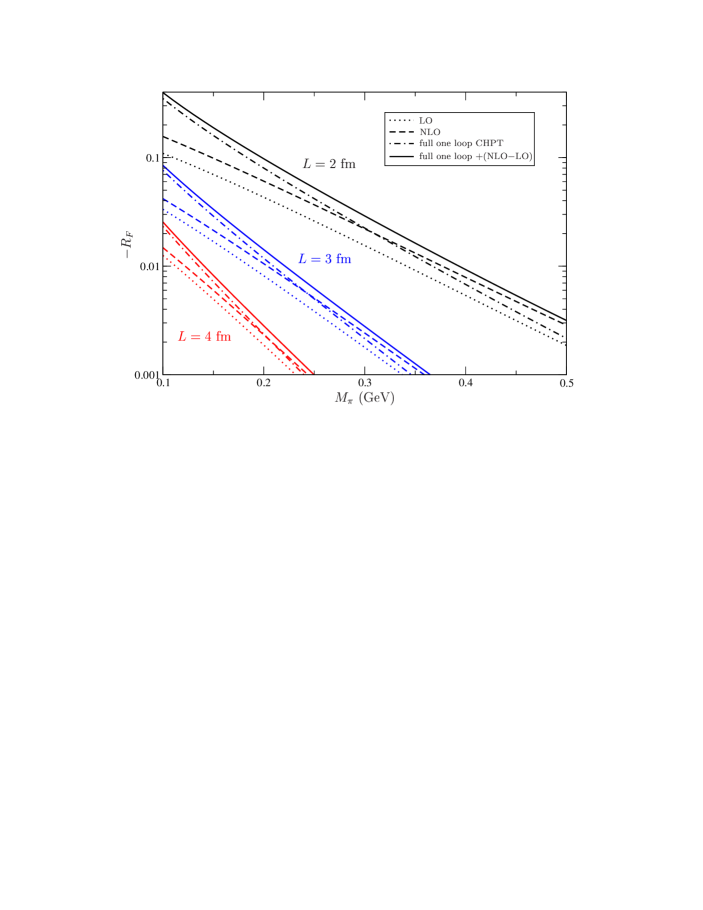
Figure 2: The absolute value of the relative finite volume correction $R_{F}=F_{\pi,L}/F_{\pi}-1$ as a function of $M_{\pi}$ for different volume sizes. We plot the leading (LO) and next-to-leading order (NLO) in the chiral expansion of the asymptotic formula (18) and also the full one-loop result in CHPT (24). The solid lines show the sum of the full one-loop result and the NLO correction in the asymptotic formula.

In comparison to the pion mass, the finite volume corrections in Eq. (24) are a factor 4 larger but negative – the sign difference is in accordance with the observation that in finite volume chiral symmetry is restored, i.e. the pion becomes heavier and its decay constant tends to vanish. Apart from this quantitative difference, the numerical analysis gives results which are qualitatively similar to those obtained for the pion mass [2]:

1. the finite volume corrections are exponentially suppressed for large values of $M_{\pi}L$ and become negligible rather quickly;

2. the leading term in the chiral expansion of the asymptotic formula receives large corrections even for the physical values of the quark masses – the similarity to the pion mass results makes us however think that the series will start to show a convergent behaviour at NNLO;

3. the leading term in the asymptotic expansion also receives large corrections from the subleading ones whenever the finite volume effects are nonnegligible;

4. since subleading terms are important both in the chiral as well as in the asymptotic expansion, the best estimate of the size of these finite-volume corrections is obtained by summing the subleading effects in both expansions, as shown by the solid curves in Fig. 2.

For example, in a recent calculation of $F_{\pi}$ on the lattice [11] with dynamical fermions a volume of $L=2.5$ fm size has been used, and pion masses as low as $0.24$ GeV. For these values the finite volume corrections evaluated with the asymptotic formula to NLO (LO) are 1.5% (1.1%), whereas the full one-loop calculation gives 1.6%. Adding both types of subleading effects we find a total correction of 2%. In Ref. [12], $L=1.5$ fm and $M_{\pi}=0.4$ GeV were used: in this case the full one-loop calculation gives a 3.4% effect, whereas adding the NLO chiral corrections we get to 4.5%. For the parameters used in [13] finite-volume effects are negligible.

6. Conclusions

We have derived an asymptotic formula for the pion decay constant in a finite large volume along the same lines as Lüscher’s formula for the pion mass [4]. The advantage offered by such a formula is a relatively easy access to a study of higher order chiral corrections in finite volume effects. We have evaluated these numerically and have shown that in $F_{\pi}$ these corrections are large, analogously to what has been found for $M_{\pi}$ [2]. In the present case we could use existing calculations of the relevant infinite-volume amplitude to evaluate next-to-leading chiral corrections. Going one order higher in this expansion would require the calculation of the $\langle 3\pi|A_{\mu}|0\rangle$ amplitude to two loops in CHPT.

The asymptotic formula derived here immediately applies (after the necessary but obvious modifications) to other similar quantities, like $G_{\pi}$. As we have explicitly verified, the asymptotic formulae for $F_{\pi}$ and $G_{\pi}$ satisfy a Ward identity that relates their ratio to $M_{\pi}^{2}/\hat{m}$: if one extracts the finite-volume expression for $M_{\pi}$ from this Ward identity one recovers Lüscher’s formula. The formula applies also to the decay constants of heavier mesons, like $F_{K}$. In the latter case the study of these finite volume effects [9] is of direct phenomenological interest in view of the recent application of the lattice calculation of the $F_{K}/F_{\pi}$ ratio to the extraction of $V_{us}$ [10] – it is worth mentioning that for this application the required precision of the lattice result is at the percent level. The same formula can also be applied to the decay constants of yet heavier mesons, like $f_{D}$ or $f_{B}$. In this case, however, the advantage provided by the asymptotic formula with respect to a plain one-loop calculation (as recently performed in [14]) will be of practical relevance only if the knowledge of the low energy constants of the chiral Lagrangian describing the coupling of heavy mesons to pions [15] is extended beyond leading order.

References

- [1] J. Gasser and H. Leutwyler, Nucl. Phys. B 307 (1988) 763.
- [2] G. Colangelo and S. Durr, Eur. Phys. J. C 33 (2004) 543 [arXiv:hep-lat/0311023].
-
[3]
D. Becirevic and G. Villadoro,
Phys. Rev. D 69 (2004) 054010
[arXiv:hep-lat/0311028];
A. Ali Khan et al. [QCDSF-UKQCD Coll.], arXiv:hep-lat/0312030;
M. Guagnelli et al., arXiv:hep-lat/0403009;
D. Arndt and C. J. D. Lin, arXiv:hep-lat/0403012;
S. R. Beane, arXiv:hep-lat/0403015. - [4] M. Lüscher, Commun. Math. Phys. 104, 177 (1986).
-
[5]
J. Bijnens et al.,
Phys. Lett. B 374 210 (1996)
[arXiv:hep-ph/9511397],
Nucl. Phys. B 508 263 (1997) [Erratum-ibid. B 517 639 (1998)] [arXiv:hep-ph/9707291]. - [6] G. Colangelo, M. Finkemeier and R. Urech, Phys. Rev. D 54 (1996) 4403 [arXiv:hep-ph/9604279].
- [7] G. Colangelo, J. Gasser and H. Leutwyler, Nucl. Phys. B 603, 125 (2001) [arXiv:hep-ph/ 0103088].
- [8] J. Gasser and H. Leutwyler, Phys. Lett. B 184 83 (1987).
- [9] G. Colangelo and C. Haefeli, in preparation.
- [10] W. J. Marciano, arXiv:hep-ph/0402299.
-
[11]
C. T. H. Davies et al. [HPQCD Coll.],
Phys. Rev. Lett. 92 (2004) 022001
[arXiv:hep-lat/0304004];
C. Aubin et al. [MILC Coll.], arXiv:hep-lat/0309088. - [12] C. R. Allton et al. [UKQCD Coll.], arXiv:hep-lat/0403007.
- [13] F. Farchioni, I. Montvay and E. Scholz [qq+q Coll.], arXiv:hep-lat/0403014.
- [14] D. Arndt and C. J. D. Lin, in Ref. [3].
-
[15]
G. Burdman and J. F. Donoghue,
Phys. Lett. B 280, 287 (1992),
M. B. Wise, Phys. Rev. D 45 (1992) 2188.
T. M. Yan et al., Phys. Rev. D 46 (1992) 1148 [Erratum-ibid. D 55 (1997) 5851].