HU-EP-04/16
DESY 04-048
Locality with staggered fermions

Abstract

We address the locality problem arising in simulations, which take the square root of the staggered fermion determinant as a Boltzmann weight to reduce the number of dynamical quark tastes. A definition of such a theory necessitates an underlying local fermion operator with the same determinant and the corresponding Green’s functions to establish causality and unitarity. We illustrate this point by studying analytically and numerically the square root of the staggered fermion operator. Although it has the correct weight, this operator is non-local in the continuum limit. Our work serves as a warning that fundamental properties of field theories might be violated when employing blindly the square root trick. The question, whether a local operator reproducing the square root of the staggered fermion determinant exists, is left open.

1 Introduction

Traditionally two formulations of lattice QCD, Wilson [?] and staggered or Kogut-Susskind fermions [?,?], were used extensively in practical simulations. Wilson type fermions suffer from the breaking of chirality. Staggered fermions rely on the appealing idea to get rid of explicit spin degrees of freedom. They arise naturally constructing the square root of the lattice Laplace operator [?]. Massless staggered fermions have a continuous taste non-singlet U(1) axial symmetry which is dynamically broken yielding one Goldstone pion [?–?,?,?–?,?,?]. This symmetry prevents from additive mass renormalization and together with the reduced number of degrees of freedom per lattice site, these properties make staggered fermions well suitable for numerical simulations. Their “unwanted” properties are the doubling, in the continuum limit each flavor comes in four “tastes”, the breaking of the taste symmetry at finite lattice spacing and the not straightforward construction of operators.

In addition to Wilson and staggered fermions (and their improved versions) many new discretizations of fermions on the lattice have been proposed, most notably overlap fermions [?], see Ref. [?] for a recent review.

With staggered fermions many computations within the quenched approximation have been performed [?,?]. An interesting and important universality check is represented by the APE plot shown in Ref. [?] where quenched data from different fermion discretizations are compared to the continuum extrapolation of the CP-PACS collaboration data [?].

Since the early times of lattice computations staggered fermions have been simulated dynamically [?]. The doubling in four degenerate tastes in the continuum limit can be exploited since the tastes behave like quarks as far as the QCD interaction is concerned. But to describe real world QCD one needs a formulation for one or two tastes. An early attempt to describe two tastes by reducing the degrees of freedom, called the reduced staggered fermion formalism [?], although it satisfies unitarity and positivity, leads to a complex determinant [?] and it is therefore not suitable for numerical simulations. Another way of reducing the number of tastes is the so called square (or fourth) root trick [?]. It amounts of taking the square (or fourth) root of the staggered fermion determinant, motivated by its factorization in the continuum limit. While in several places warnings about its potential danger have been expressed [?,?], the central problem that this is not an ab initio formulation of lattice QCD [?,?,?] has not been addressed in the literature. Arguments based on partially quenched chiral perturbation theory [?] support the square root trick but this should only be considered as a motivation for a first principle study.

From the numerical simulation side there are no major obstacles to implement the square root trick. But as more and more results based on such simulations are being published and ambitious high precision tests of the standard model announced [?], the theoretical issues postponed so far have to be addressed. Here we only try to state the problem concerning locality, following a benchmark investigation for the overlap case in Ref. [?].

At a glance the problem discussed in this work can be introduced by the following simple arguments.

1. In the QCD partition function on the lattice only local operators appear

   $$\mathcal{Z} = \int_{U,\bar{\psi},\psi}\exp\left\{-S_{g}(U)+a^{4}\sum_{x}\bar{\psi}(x)D\psi(x)\right\}\,,$$ (1.1)

   where $S_{g}(U)$ is the gauge action in terms of gauge links $U$ and $D$ is the, assumed to be local, Dirac operator acting on fermion fields $\bar{\psi},~{}\psi$.

2. The integration over the fermion fields $\bar{\psi},~{}\psi$ generates an effective action

   $$\mathcal{Z} = \int_{U}\det(aD)\exp\left\{-S_{g}(U)\right\}=\int_{U}\exp\left\{-S_{g}(U)+{\rm tr}\ln(aD)\right\},$$ (1.2)

   which is non-local in the gauge link variables.

The non-locality of the effective action does not mean a non-locality of the theory if the latter possesses an underlying local formulation in terms of fundamental degrees of freedom.

If the starting point of a lattice theory is eq. (1.2), e.g. with the effective action

$$S_{\rm eff} = -S_{g}(U)+\frac{1}{2}{\rm tr}\ln(aM)$$ (1.3)

corresponding to the Boltzmann weight $\sqrt{\det(aM)}$, then an equivalent formulation like in eq. (1.1) in terms of a local operator $D$ is needed in order to establish causality and discuss renormalizability and universality.

The present work is organized as follows. In Section 2 we formulate precisely the locality problem related to the square root trick. We present our “candidate” for a local operator $D$ namely the most naive choice, which is to take the square root of the staggered operator. In Section 3 we present our analytical results, in particular in the free field theory where the square root operator is proven to be non-local. Numerical investigations are still of interest to establish the actual “non-localization” range in the interacting theory. Section 4 presents the simulation results in the quenched approximation. We discuss these results in Section 5. There are three appendices devoted to the derivation of our analytical results and to the study of finite size effects in our simulations.

2 Formulation of the problem

We consider an Euclidean hypercubic lattice with lattice spacing $a$ and coordinates $x_{\mu}=n_{\mu}a$ with $n_{\mu}=0,1,\ldots,L/a-1$. The number of sites in each direction is $L/a$ and it is assumed to be even. The directions are denoted by $\mu=0,1,2,3$ and $a_{\mu}$ is a displacement vector by one lattice spacing along the $\mu$ direction. The action for Kogut-Susskind staggered fermions is

$$S = S_{g}(U)-a^{4}\sum_{x}\bar{\chi}(x)M\chi(x)$$ (2.4)

$$M\chi(x) = m\chi(x)+\sum_{\mu}\frac{1}{2a}\eta(x,\mu)\left[U(x,\mu)\chi(x+a_{\mu})-U^{\dagger}(x-a_{\mu},\mu)\chi(x-a_{\mu})\right]\,,$$

where $\eta(x,\mu)=(-1)^{\sum_{\nu<\mu}n_{\nu}}$ are the staggered phases. The fermion field $\chi$ has only SU(3) color indices. Periodic boundary conditions are used for the gauge field and (anti-)periodic for the fermion field. In the continuum limit $M$ exhibits spectrum doubling since it describes four degenerate “tastes”, which can be interpreted as four flavors of quarks [?,?–?,?]. At finite lattice spacing there are O($a^{2}$) taste-changing interactions even in the free theory. The main advantage of staggered fermions is that the action eq. (2.4) is invariant for $m=0$ under the continuous taste non-singlet U(1) axial transformation

$$\chi(x)\to{\rm e}^{i\beta\epsilon(x)}\chi(x)\,,\qquad\bar{\chi}(x)\to{\rm e}^{i\beta\epsilon(x)}\bar{\chi}(x)\,,$$ (2.5)

where

$$\epsilon(x) = (-1)^{\sum_{\mu}n_{\mu}}\,,$$ (2.6)

from which it follows that there is no additive mass renormalization [?,?].

The question, whether there exists a formulation for two degenerate tastes of staggered fermions has been considered in Ref. [?]. In this so called reduced staggered fermion formalism the fermion field $\chi$ lives on odd sites only and the anti-fermion field $\bar{\chi}$ on even sites only (“even” and “odd” being defined by the sign of $\epsilon(x)$ eq. (2.6)). Although this theory satisfies unitarity and positivity it leads to a complex fermion determinant [?] and is therefore not suitable for numerical Monte Carlo studies. Also this reduced formalism does not have any continuous U(1) axial symmetry [?,?].

The authors of Ref. [?] proposed to take the square (or fourth) root of the fermion determinant to reduce the number of tastes from four to two (or one). Based on the factorization in the naive continuum limit

$$\det(aM) \stackrel{{\scriptstyle a\to 0}}{{\longrightarrow}} \det(a\Omega)^{4}$$ (2.7)

in terms of a one-flavor fermion operator $\Omega$, taking the square root amounts to quenching two out of four tastes and this idea seems to work out in partially quenched chiral perturbation theory [?].

The square (and fourth) root trick is employed in large scale simulations by the MILC [?] and JLQCD [?] collaborations. From the algorithmic side the square root of the determinant can be dealt with the R algorithm [?], with the PHMC algorithm [?,?] or with the RHMC algorithm [?]. In the computation of quark propagators the original four taste staggered operator is used. Correlation functions are built using sources that project onto the desired valence taste components [?]. This is justified in partially quenched chiral perturbation theory with some complication for taste-singlet operators [?]. However the danger with such an approach are possible unitarity violations through a mismatch of sea and valence quark lines. This fundamental question, which deserves more investigation, is not addressed in the present work.

In order to establish causality and universality for the theory implicitly defined by taking the square root of the staggered fermion determinant, a local definition of the theory from first principles like in eq. (1.1) is needed. Explicitly the problem is to find a fermion operator $D$ such that

$$\det(aD)=\sqrt{\det(aM)} \|G(x,y)\|\leq C{\rm e}^{-\gamma\|x-y\|_{\rm E}/a}\,,$$ and (2.8)

with $C$ and $\gamma>0$ independent of $U$ [?,?]. In eq. (2.8) $\|G(x,y)\|$ is the operator norm of the kernel

$$aD\psi(x) = a^{4}\sum_{y}G(x,y)\psi(y)$$ (2.9)

and $\|x-y\|_{\rm E}$ is the Euclidean norm.

A technical point is that so far we have used $M$ as the operator describing four tastes. In numerical simulations the fermion determinant is represented by pseudofermions and for this the Hermitean positive definite operator $M^{\dagger}M$ is needed, which describes eight tastes. The number of tastes can be reduced to the original four by noting that $M^{\dagger}M$ decouples the even and the odd sublattices and that [?]

$$\det(aM) = \det(a^{2}(M^{\dagger}M)_{e})=\det(a^{2}(M^{\dagger}M)_{o})\,.$$ (2.10)

In eq. (2.10) the subscripts for $(M^{\dagger}M)_{e}$ and $(M^{\dagger}M)_{o}$ refer to the operator $M^{\dagger}M$ acting on fields living only on the even or odd sublattices respectively. In the following to describe four tastes of staggered fermions the operator $(M^{\dagger}M)_{e}$ is used.

In this work we investigate the locality properties of the so far only known candidate for an operator $D$ to satisfy eq. (2.8), namely

$$D = \sqrt{(M^{\dagger}M)_{e}}\,,$$ (2.11)

where the operator square root is obtained by a Chebyshev polynomial approximation [?–?]. It approximates the unique [?–?] Hermitean positive definite square root of $(M^{\dagger}M)_{e}$.

3 Analytical results

3.1 Bound

To derive a bound on the locality of the operator $D$ defined in eq. (2.11) we need to know the spectral bounds of $M^{\dagger}M$ [?]. In the free theory

$$a^{2}M^{\dagger}M{\rm e}^{ipx} = [(am)^{2}+\sum_{\mu}\sin^{2}(p_{\mu}a)]{\rm e}^{ipx}$$ (3.12)

which implies for the spectrum ${\rm spec}(a^{2}M^{\dagger}M)\subset[(am)^{2},4+(am)^{2}]$. In the interacting case the upper bound is lifted

$${\rm spec}(a^{2}M^{\dagger}M) \subset [u,v]\,,\quad u=(am)^{2}\,,\quad v=16+(am)^{2}\,.$$ (3.13)

The operator $(M^{\dagger}M)_{e}$ has the same spectral bounds [?].

In order to handle analytically the operator $D$ we would like to use the series of polynomials $S_{n}(z)$ of degree $n$ defined by the generating function

$$\sqrt{1+t^{2}-2tz} = \sum_{n=0}^{\infty}S_{n}(z)t^{n}\,.$$ (3.14)

Properties of this series (where $z$ is a number) are discussed in the Appendix A. Following Ref. [?] we define the operator (with obvious insertions of unit matrices)

$$z = \frac{v+u-2a^{2}(M^{\dagger}M)_{e}}{v-u}\,,$$ (3.15)

which maps the spectrum $[u,v]$ of $a^{2}(M^{\dagger}M)_{e}$ into $[-1,1]$. We then set

$$t={\rm e}^{-\theta} \cosh\theta=\frac{v+u}{v-u}\,,\quad\theta>0\,.$$ with (3.16)

For this choice of $t$ we have

$$1+t^{2}-2tz = \frac{4{\rm e}^{-\theta}}{v-u}a^{2}(M^{\dagger}M)_{e}$$ (3.17)

and we can use eq. (3.14) to provide a series expansion for the operator $D$.

The kernel $G(x,y)$ eq. (2.9) of the square root operator can be expressed in terms of the kernels $G_{n}(x,y)$ for the polynomial operators $S_{n}(z)$. From eq. (3.14) and eq. (3.16) we get

$$G(x,y) = \frac{1}{2}\sqrt{v-u}{\rm e}^{\theta/2}\sum_{n=0}^{\infty}G_{n}(x,y){\rm e}^{-n\theta}$$ (3.18)

Since $z$ as it is defined in eq. (3.15) connects two neighboring even sites on the lattice, we have

$$G_{n}(x,y)=0 n<n_{\rm min}=\frac{\|x-y\|_{1}}{2a}\,,$$ for

where $\|x-y\|_{1}/a$ is the number of links between $x$ and $y$ (“taxi driver distance”). In eq. (A.43) a bound for the remainder of the polynomial series in eq. (3.14) truncated after $n=n_{\rm min}-1$ terms is given. Since the spectrum of $z$ eq. (3.15) is contained in $[-1,1]$ and using the operator calculus, the bound eq. (A.43) implies

$$a^{4}\|G(x,y)\| \leq \frac{\sqrt{v-u}}{(n_{\rm min}-1)\pi}{\rm e}^{\theta/2}{\rm e}^{-\|x-y\|_{1}/(2a/\theta)}\,,\quad n_{\rm min}\geq 2$$ (3.19)

for the norm of the kernel $G(x,y)$ in SU(3) color space. Inserting the values for the spectral bounds given in eq. (3.13) into the definition of $\theta$ eq. (3.16) we obtain

$$\theta = \frac{am}{2}+{\rm O}((am)^{3})\,.$$ (3.20)

This means that $a^{4}\|G(x,y)\|$ is bounded by an exponential $\propto\exp(-r/r_{\rm loc})$ with $r=\|x-y\|_{1}$ and

$$r_{\rm loc} = \frac{2a}{\theta}\simeq\frac{4}{m}\,.$$ (3.21)

The localization range $r_{\rm loc}$ stays finite in the continuum limit. This is in contradiction to a local theory where we need $r_{\rm loc}$ proportional to the lattice spacing.

The result eq. (3.19) represents an upper bound on the localization of the operator $D$, the theory could in principle still be local in the continuum. We devote therefore our attention to the free theory where we can achieve an exact result. Since in the free theory $\theta=am+{\rm O}((am)^{3})$, the bound eq. (3.19) gives $r_{\rm loc}^{({\rm free})}\simeq 2/m$.

3.2 Exact result in the free theory

We consider an infinite lattice. The free operator $M^{\dagger}M$ decouples on sixteen sublattices of lattice spacing $2a$ where it acts like a Laplace operator. The Fourier transformation of the square root of the diagonal operator in momentum space eq. (3.12) yields for the kernel $G(x,y)$ eq. (2.9)

$$G(x,y) = \int_{-\pi/(2a)}^{\pi/(2a)}\frac{d^{4}p}{\pi^{4}}\sqrt{(am)^{2}+\sum_{\mu}\sin^{2}(p_{\mu}a)}\,{\rm e}^{ip(x-y)}\,,$$ (3.22)

where $(x_{\mu}-y_{\mu})/a$ is even for all $\mu$, that is $x$ and $y$ live on one of the sixteen sublattices of lattice spacing $2a$. Clearly then eq. (3.22) applies also for $D$ in eq. (2.11). This integral is solved in Appendix B and the result (for $y=0$) is given by replacing $a$ with $2a$ in eq. (B.48).

The continuum version of eq. (3.22) is also computed in Appendix B, the result is eq. (B.53)

$$\int_{-\infty}^{\infty}\frac{d^{4}p}{(2\pi)^{4}}\sqrt{p^{2}+m^{2}}\,{\rm e}^{ipx}=$$

$$-\frac{1}{4\pi^{2}}\frac{m^{2}}{\|x\|_{\rm E}^{3}}\left(1+\frac{3}{m\|x\|_{\rm E}}+\frac{3}{m^{2}\|x\|_{\rm E}^{2}}\right){\rm e}^{-m\|x\|_{\rm E}}\,.$$ (3.23)

As is shown in Appendix B the continuum and lattice results agree at large Euclidean distance and this establishes that the operator $D$ in eq. (2.11) is non-local in the free continuum limit. The localization range is $r_{\rm loc}=1/m$. By noting that $\|x\|_{\rm E}\leq\|x\|_{1}\leq 2\|x\|_{\rm E}$ we see that the bound eq. (3.19) in the free theory is saturated.

It is very unlikely that the introduction of gauge interactions changes qualitatively this result. From the numerical point of view it is still interesting to investigate what actually happens in the interacting theory. Because of confinement the quark mass will be “replaced” in the bound eq. (3.21) by some hadronic mass, which could be very large in a favorable case. From a similar study in the overlap case [?] it is known that the analytical bound is only poorly saturated.

4 Numerical results

To test numerically the locality of the operator $D$ eq. (2.11) we follow closely Ref. [?]. We consider hypercubic lattices with $L/a$ sites in each direction and periodic boundary conditions. The operator $D$ acts on fields living on the even sites only. We define the source field

$$\xi_{c}(x) = \left\{\begin{array}[]{ll}1&\mbox{if $x=y$ and $c=1$}\\ 0&\mbox{otherwise}\,,\end{array}\right.$$ (4.26)

where $y$ is the location of the source and $c$ runs over the color index of the field. We take a point-like color source because we are only interested in the decay properties of

$$\psi(x) = aD\xi_{c}(x)$$ (4.27)

described in terms of the function

$$f(r) = \max\big{\{}\|\psi(x)\|\,\big{|}\,\|x-y\|_{1}=r\big{\}}\,.$$ (4.28)

A different choice of the source in eq. (4.26), e.g. spread in a $2^{4}$ hypercube describing “one” taste will not change the result, which concerns a mathematical property of the operator that needs to be fulfilled. In eq. (4.28) $\|\psi(x)\|$ is the SU(3) color norm and the “taxi driver distance” is defined as

$$\|x-y\|_{1} = \sum_{\mu}\min\left\{|x_{\mu}-y_{\mu}|,L-|x_{\mu}-y_{\mu}|\right\}\,.$$ (4.29)

Hence $\|x-y\|_{1}/a$ is the number of links for the shortest path on the lattice between $x$ and $y$ using the periodicity. The maximal value that $\|x-y\|_{1}$ can take is $2L$. The taxi driver distance is used here since it arises naturally in the derivation of the analytic bound eq. (3.21).

$\beta$	$am$	$r_{0}m_{\rm G}$	$L/a$	$\varepsilon$	pol. degree	#configs.
6.0	0.01	1.29 [?]	16	$2\times 10^{-7}$	490	200
			24,32	$8\times 10^{-9}$	735	600
6.2	0.007	1.34(4) [?]	24	$4\times 10^{-9}$	1050	150
			36	$4\times 10^{-9}$	1050	300
6.5	0.005	1.27(1) [?]	32	$2\times 10^{-9}$	1470	300
			48	$2\times 10^{-9}$	1470	192

Table 1: Simulation parameters. The last three columns tabulate the relative accuracy $\varepsilon$ eq. (4.30), the degree of the polynomial and the number of configurations generated.

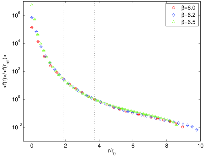
Figure 1: Decay of $\langle f(r)\rangle$ defined in eq. (4.28). The curves are normalized to be 1 at the distance $r_{\rm ref}/r_{0}=3.72$ corresponding to the location of the rightmost vertical dotted line.

We compute the function $f(r)$ on configurations generated in the quenched approximation and denote the average in the quenched ensemble by $\langle f(r)\rangle$. We keep the location of the source fixed at $y=0$, the average over gauge configurations projects onto the gauge invariant part of eq. (4.28). Table 1 summarizes the simulation parameters. We simulate at three $\beta$ values in order to take the continuum limit. The quark masses are obtained from the literature [?,?,?] and define a line of constant physics where the mass $m_{\rm G}$ of the Goldstone pion $\pi_{\rm G}$ is $r_{0}m_{\rm G}=1.30(3)$ in units of the hadronic scale $r_{0}$ [?,?]. We have two approximately matched physical volumes $Lm_{\rm G}\approx 4$ and $Lm_{\rm G}\approx 6$ at all $\beta$ values. At $\beta=6.0$ we also have a third larger volume, which we used to study the finite volume effects. Statistical errors of derived quantities were determined by the method of Ref. [?].

We implemented the Chebyshev polynomial approximation using the Clenshaw’s recurrence formula [?–?]. As can be seen from Table 1 for most of the computations a relative accuracy $\varepsilon=10^{-8}-10^{-9}$ was required, which is defined as

$$\varepsilon=\frac{\|(D^{2}-(M^{\dagger}M)_{e})R\|}{\|(M^{\dagger}M)_{e}R\|}$$ (4.30)

where $R$ is a normalized Gaussian random vector $R$.

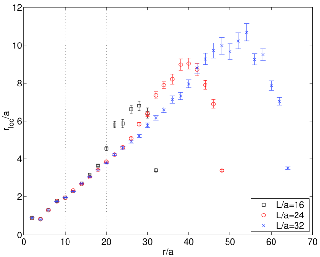
Figure 2: Effective localization ranges $r_{\rm loc}(r)$ at $\beta=6.0,\;am=0.01$ for different volumes. The vertical dotted lines correspond to distances from the source smaller than the minimal distances $\;r_{\rm min}(L)\approx L\;$ at which finite volume effects for $L/a=16,\;24$ become sizeable.

In Fig. 1 we show in a semilogarithmic plot the results for $\langle f(r)\rangle$ as function of the taxi driver distance $r$ in units of $r_{0}$ at the three different $\beta$ values for the volume $Lm_{\rm G}\approx 6$. For a better comparison of the curves we normalized $\langle f(r)\rangle$ by the (linearly interpolated) value $\langle f(r_{\rm ref})\rangle$, where the physical distance $r_{\rm ref}/r_{0}=3.72$ corresponds to the rightmost vertical dotted line. Fig. 1 shows remarkable scaling as the continuum limit is approached, which means that there is a physical scale of “non-localization” $r_{\rm loc}$.

For small distances $r\ll\Lambda_{\rm QCD}^{-1}$ the form of $\langle f(r)\rangle$ is dictated by perturbation theory and it is expected to follow the polynomial (in $1/r$) result in the free theory eq. (3.23). For large distances $r$ we assume

$$\langle f(r)\rangle \propto {\rm e}^{-r/r_{\rm loc}(r)}\,.$$ (4.31)

The inverse localization range $r_{\rm loc}(r)^{-1}$ can be computed by taking two consecutive values of $r$ to extract the exponential. The results for three volumes at $\beta=6.0$ are shown in Fig. 2. It is clear that the decay of $\langle f(r)\rangle$ is not described by a single exponential. On each of the volumes $r_{\rm loc}(r)$ has a “bump” for large taxi driver distances, which becomes higher as the volume gets larger. This is a finite volume effect and is discussed in Appendix C.

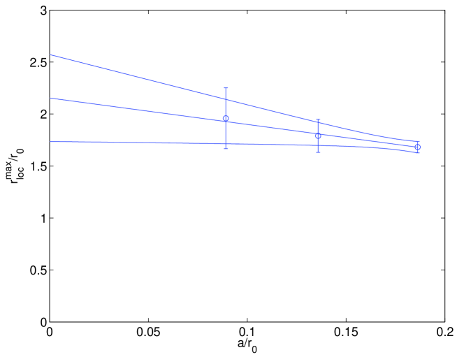
Figure 3: The continuum limit of the upper bound on the localization range in the volume $Lm_{\rm G}\approx 6$.

We adopt two strategies to define a localization range of the operator $D$ in the continuum limit. The first is to take for the physical volume $Lm_{\rm G}\approx 6$ the largest value of $r_{\rm loc}(r)$, which we denote by $r_{\rm loc}^{\rm max}$, at each $\beta$ value. Changing the volume will slightly change this value but the volume $Lm_{\rm G}\approx 6$ can be considered typical for present quenched simulations. The results are shown in Fig. 3 and give a continuum limit value

$$\frac{r_{\rm loc}^{\rm max}}{r_{0}} = 2.15(42)\quad\mbox{for}\quad Lm_{\rm G}\approx 6\,,$$ (4.32)

or $r_{\rm loc}^{\rm max}m_{\rm G}=2.8(6)$. Compared to the analytic bound given in eq. (3.21) the values of $r_{\rm loc}^{\rm max}$ that we obtain at the three $\beta$ values are about 40 times smaller. The fact that the analytic bound is poorly saturated is in agreement with similar observations made in Ref. [?].

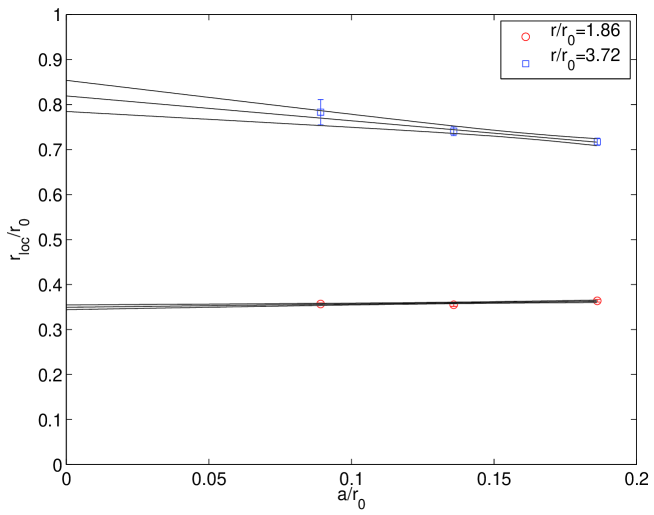
Figure 4: The continuum limit of the localization range computed at two constant physical distances from the source.

The second strategy is to compute the localization range at a physical value of the taxi driver distance from the source. We take two distances, $r/r_{0}=1.86$ and twice this value $r/r_{0}=3.72$, which are marked in Fig. 1, Fig. 2 and Fig. 7 by the vertical dotted lines. At $\beta=6.0$ there are no finite size effects in $r_{\rm loc}(r)$ computed at these two distances on lattices of size $L/a=24$ ($Lm_{\rm G}\approx 6$), as can be seen by comparing to results on the larger volume $L/a=32$ in Fig. 7. For $r_{\rm loc}(r/r_{0}=1.86)$ we checked at the other $\beta$ values that already in the volume $Lm_{\rm G}\approx 4$ there are no finite size effects. We take the lattice volume $Lm_{\rm G}\approx 6$ and perform a linear interpolation of $r_{\rm loc}(r)$ to get its values at the desired distances for the three $\beta$ values. We obtain the results shown in Fig. 4 giving the continuum limit values

$$\frac{r_{\rm loc}(r/r_{0}=1.86)}{r_{0}} = 0.350(5)\,,$$ (4.33)

$$\frac{r_{\rm loc}(r/r_{0}=3.72)}{r_{0}} = 0.819(35)\,,$$ (4.34)

or $r_{\rm loc}(r/r_{0}=1.86)m_{\rm G}=0.455(12)$ and $r_{\rm loc}(r/r_{0}=3.72)m_{\rm G}=1.06(5)$. We remind that a local operator would imply $r_{\rm loc}(r)={\rm O}(a)$ for all distances $r$.

5 Conclusions

We have studied the locality problem for a theory defined by taking the square root of the staggered fermion operator. In terms of the fundamental fermion fields, this operator needs to be local in order to prove causality and unitarity of the so defined theory. In our work, we proved that in the free field limit such a theory is non-local at the scale of the inverse quark mass. Adding gauge fields, simulations in the quenched approximation have revealed that the “non-localization” range is of the order of the inverse Goldstone pion mass in the continuum limit. We do not expect that taking the square root of staggered fermion operators constructed with improved actions such as Asqtad [?] or HYP [?] will change qualitatively and even quantitatively the situation, since smearing makes configurations even closer to the free case.

How can we interpret our results, also in the context of present day simulations? We have studied a candidate theory for two tastes of staggered fermions obtained by taking the square root of the staggered fermion operator in the action and the corresponding Green’s functions. Our work shows that such a theory is non-local in the continuum limit at the scale of the Goldstone pion Compton wavelength, i.e. the lightest particle in the theory. Hence this solution of the “two taste problem” leads to an unacceptable field theory that has to be dismissed. This leaves the question open, of course, whether there exists a local operator $D$, which provides a Boltzmann weight equal to the square root of the staggered fermion determinant.

Present dynamical staggered fermion simulations do not use this setup since only the square root of the determinant is employed. The corresponding action $S=1/2{\rm tr}\ln(M^{\dagger}M)_{e}$ is simulated with the R algorithm [?] with the zero step-size limit or $S=-\phi^{\dagger}((M^{\dagger}M)_{e})^{-1/2}\phi$ in terms of a pseudofermion field $\phi$ with an exact algorithm [?,?]. We emphasize that these simulations generate the correct Boltzmann weight since the non-local bosonic formulation is only a technical trick to perform the numerical simulations. If a local operator $D$ reproducing the square root of the staggered fermion determinant is found then the configurations generated by present algorithms are safe.

There still remains, however, the problem of unitarity. The point is a mismatch between the operators used for valence and sea quarks. The valence quarks are discretized through the four taste staggered operator, while the sea quarks would be introduced through the “still to be found” two taste local operator $D$. We believe that at this point the recovery of the optical theorem is an open problem, which needs a clarification. The operator $D$, acting on the fundamental fermion fields, should dictate which are the appropriate Green’s functions for a two taste theory. The Green’s functions that are used at present are most likely not the ones that correspond to the local operator $D$.
Acknowledgements: We thank A. Alexandru, T. DeGrand, A. Hasenfratz, P. Hasenfratz, R. Hoffmann, A. Kronfeld, M. Lüscher, F. Niedermayer and U. Wolff for precious discussions and suggestions. The simulations in the present work have been carried out using the MILC collaboration’s public lattice gauge theory code. We also thank the computer center at DESY Zeuthen and Humboldt University for their professional assistance.

Appendix A A polynomial expansion of the square root

Consider the generating function of the Gegenbauer polynomials $C_{n}^{\gamma}(z)$

$$(1+t^{2}-2tz)^{-\gamma} = \sum_{n=0}^{\infty}t^{n}C_{n}^{\gamma}(z)$$ (A.35)

They are defined for any (fixed) $\gamma\in\mathbb{C}$. Their natural domain is $z\in[-1,1]$. Many details about Gegenbauer polynomials can be found in [?], section 10.9. We only list the recursion and a bound:

$$(n+1)C_{n+1}^{\gamma}(z) + (n+2\gamma-1)C_{n-1}^{\gamma}(z)\;=\;2(n+\gamma)\,zC_{n}^{\gamma}(z)$$ (A.36)

$$|C_{n}^{\gamma}(z)| \leq \left(n+2\gamma-1\atop n\right)\qquad\gamma>0$$ (A.37)

The power series (A.35) converges for $|t|<1$. This may be used as a starting point for fractional inversion[?]. Here we specialize to the case of $\gamma=-1/2$, which provides an expansion of the square root:

$$\sqrt{1+t^{2}-2tz} = \sum_{n=0}^{\infty}t^{n}S_{n}(z)$$ (A.38)

$$S_{n}(z) \equiv C_{n}^{-1/2}(z)$$

The first few polynomials $S_{n}(z)$ are

$$S_{0}(z) = 1$$

$$S_{1}(z) = -z$$

$$S_{2}(z) = \frac{1}{2}(1-z^{2})$$

We find $S_{n}(\pm 1)=0$ for $n\geq 2$. In fact the recursion (A.36) allows us to prove the useful relation

$$S_{n}(z) = \frac{1-z^{2}}{n(n-1)}\;C_{n-2}^{3/2}(z)\qquad n\geq 2$$ (A.39)

As an immediate consequence, the bound (A.37) provides the estimate

$$|S_{n}(z)| \leq \frac{1}{2}\qquad n\geq 2$$ (A.40)

In applications of the expansion (A.38), there is particular interest in the remainder $\Omega_{n}(z)$ of the series truncated after the term $\sim t^{n}$

$$\Omega_{n}(z) = \sum_{k=n+1}^{\infty}t^{k}S_{k}(z)$$ (A.41)

A simple (uniform) estimate follows immediately with the aid of (A.40):

$$|\Omega_{n}(z)| \leq \frac{1}{2}\sum_{k=n+1}^{\infty}|t|^{k}=\frac{1}{2}\frac{|t|^{n+1}}{1-|t|}\qquad n\geq 1$$ (A.42)

The coefficient of $|t|^{n+1}$ diverges as $|t|\to 1$.

We will prove the stronger (and more realistic) bound

$$|\Omega_{n}(z)| \leq \frac{2}{n\pi}\;|t|^{n+1}\qquad n\geq 1$$ (A.43)

for $z\in[-1,1]$ and $t\in(-1,1)$.

Assume $t\in(0,1)$ and let $z=\cos\phi$. The relation (A.39) translates the integral representation of $C_{n}^{3/2}$ ([?], section 10.9, eq.(31)) into

$$S_{n}(\cos\phi) = \sin^{2}\phi\,\int_{0}^{\pi}\frac{d\varphi}{\pi}\,\sin^{2}\varphi\,(\cos\phi+i\sin\phi\cos\varphi)^{n-2}\qquad n\geq 2$$

This allows us to perform the summation in $\Omega_{n}(z)$ eq.(A.41) (if $n\geq 1$)

$$\Omega_{n}(\cos\phi) = \sin^{2}\phi\;t^{n+1}\int_{0}^{\pi}\frac{d\varphi}{\pi}\,\sin^{2}\varphi\,\frac{(\cos\phi+i\sin\phi\cos\varphi)^{n-1}}{1-t(\cos\phi+i\sin\phi\cos\varphi)}$$

At the end points of the integration, the denominator takes values $1-te^{\pm i\phi}\equiv\rho e^{\mp i\delta}$, i.e. we reparametrize $(t,\phi)\to(\rho,\delta)$, with $\rho>0$ and $\delta\in[0,\pi/2)$

$$\rho = |1-te^{i\phi}|=\sqrt{1+t^{2}-2t\cos\phi}$$

$$\cos\delta = (1-t\cos\phi)/\rho$$ (A.44)

$$\sin\delta = (t\sin\phi)/\rho$$

$$\Rightarrow\quad\Omega_{n}(\cos\phi) = t^{n-1}\,\rho\sin^{2}\delta\int_{0}^{\pi}\frac{d\varphi}{\pi}\,\sin^{2}\varphi\,\frac{(\cos\phi+i\sin\phi\cos\varphi)^{n-1}}{\cos\delta-i\sin\delta\cos\varphi}$$

Rewrite this as a contour integral over $u$:

$$u \equiv \cos\delta-i\sin\delta\cos\varphi$$

$$\Rightarrow\quad 1-\rho u = t(\cos\phi+i\sin\phi\cos\varphi)$$

$$\Rightarrow\quad\Omega_{n}(\cos\phi) = \rho\int_{e^{-i\delta}}^{e^{i\delta}}\frac{du}{\pi iu}\,\sqrt{1+u^{2}-2u\cos\delta}\;(1-\rho u)^{n-1}$$

$$= \rho\int_{e^{-i\delta}}^{e^{i\delta}}\frac{du}{\pi iu}\,Q(u)\;(1-\rho u)^{n-1}$$

$$\mbox{with}\quad Q(u) \equiv \sqrt{1+u^{2}-2u\cos\delta}$$

$$= \sqrt{(u-e^{i\delta})(u-e^{-i\delta})}$$

The cut of the square root is chosen on the negative real axis. $Q(u)$ has branch points at $u=e^{\pm i\delta}$, with vertical cuts going out to $\pm i\infty$. The contour of integration connects the two branch points across the real axis.
Integrate by parts, using $Q(u)=0$ at the end points:

$$\Omega_{n}(\cos\phi) = \frac{1}{n}\int_{e^{-i\delta}}^{e^{i\delta}}\frac{du}{\pi i}\,\left(\frac{d}{du}\frac{Q(u)}{u}\right)\;(1-\rho u)^{n}$$ (A.45)

This integral is finally evaluated along the circle

$$u(\varphi) = \frac{1+e^{2i\varphi}}{2\cos\delta}\;=\;\frac{\cos\varphi}{\cos\delta}\,e^{i\varphi}\qquad\varphi\in[-\delta,\delta]$$

$$\Rightarrow\quad Q(u) = \frac{e^{i\varphi}}{\cos\delta}\sqrt{\cos^{2}\varphi-\cos^{2}\delta}$$

$$\Rightarrow\quad\frac{Q(u)}{u} = \frac{\sqrt{\cos^{2}\varphi-\cos^{2}\delta}}{\cos\varphi}$$

$$\Rightarrow\quad\Omega_{n}(\cos\phi) = \frac{1}{n\pi i}\int_{-\delta}^{\delta}d\varphi\,\left(\frac{d}{d\varphi}\,\frac{\sqrt{\cos^{2}\varphi-\cos^{2}\delta}}{\cos\varphi}\right)[1-\rho u(\varphi)]^{n}$$

Along the contour of integration,

$$|1-\rho u(\varphi)| \leq t$$

Furthermore, $Q(u)/u$ is an even function of $\varphi$, which vanishes at the end points and reaches a maximum of $\sin\delta$ in the middle. In this way we estimate

$$|\Omega_{n}(\cos\phi)| \leq \frac{t^{n}}{n\pi}\int_{-\delta}^{\delta}d\varphi\,\left|\frac{d}{d\varphi}\,\frac{\sqrt{\cos^{2}\varphi-\cos^{2}\delta}}{\cos\varphi}\right|$$

$$\leq \frac{2t^{n}}{n\pi}\,\sin\delta$$

Inspection of (A.44) shows that $\sin\delta\leq t$, which proves (A.43) for $t\in(0,1)$.

The case of $t\in(-1,0)$ follows due to the invariance of $\Omega_{n}(z)$ w.r.t. $t\to-t,z\to-z$.

Appendix B The square root in the free case

B.1 Lattice computation

On an infinite lattice in $d$ dimensions (lattice spacing $a$), we study functions of the operator (matrix)

$$m^{2}-\Delta$$ (B.46)

which reads in momentum space:

$$\left(m^{2}-\Delta\right)(p) = m^{2}+\sum_{\mu}2a^{-2}(1-\cos ap_{\mu})$$

$$= m^{2}+\sum_{\mu}\frac{4}{a^{2}}\sin^{2}\frac{ap_{\mu}}{2}$$

$$-\pi/a\leq p_{\mu}\leq\pi/a$$

Start from the ”generalized propagator” with $s\in\mathbb{C}$:

$$\left(m^{2}-\Delta\right)^{-s}(x) = a^{2s}\,\int_{-\pi/a}^{\pi/a}\frac{d^{d}p}{(2\pi)^{d}}\;\frac{e^{ipx}}{[a^{2}m^{2}+\sum_{\mu}2(1-\cos ap_{\mu})]^{s}}$$

Use the standard trick (valid for $A>0$ and $\mbox{Re}\,s>0$)

$$A^{-s} = \frac{1}{\Gamma(s)}\int_{0}^{\infty}dt\,t^{s-1}e^{-tA}$$

to factorize the $p$ integrations. They lead to modified Bessel functions of the first kind $I_{n}$:

$$\int_{-\pi/a}^{\pi/a}\frac{dp_{\mu}}{2\pi}\exp\{ip_{\mu}x_{\mu}+2t\cos ap_{\mu}\} = a^{-1}I_{x_{\mu}/a}(2t)$$

$$\Rightarrow\quad\left(m^{2}-\Delta\right)^{-s}(x) = \frac{a^{2s-d}}{\Gamma(s)}\int_{0}^{\infty}dt\,t^{s-1}e^{-t(a^{2}m^{2}+2d)}\prod_{\mu}I_{x_{\mu}/a}(2t)$$ (B.47)

For $t\to\infty$, $I_{n}(2t)\sim t^{-1/2}e^{2t}$ and the integral converges if $m\neq 0$. In case of $m=0$, we need $\mbox{Re}\,s<d/2$.

For $t\to 0$: $I_{n}(2t)\sim t^{|n|}$. In case of $x\neq 0$, the product of Bessel functions vanishes at least linearly in $t$. As a consequence, eq.(B.47) is valid for $\mbox{Re}\,s>-1$ and can be evaluated at $s=-1/2$:

$$\left(m^{2}-\Delta\right)^{1/2}(x) = \frac{a^{-d-1}}{\Gamma(-1/2)}\int_{0}^{\infty}dt\,t^{-3/2}e^{-t(a^{2}m^{2}+2d)}\prod_{\mu}I_{x_{\mu}/a}(2t)$$ (B.48)

$$(x\neq 0)$$

(Note: $\Gamma(-1/2)=-2\sqrt{\pi}$).

For the special case of $x=0$, continuation to $s=-1/2$ requires to subtract a term in the integrand:

$$I_{0}(2t)^{d} = \left[I_{0}(2t)^{d}-1\right]+1$$

$$\int_{0}^{\infty}dt\,t^{s-1}e^{-t(a^{2}m^{2}+2d)} = \Gamma(s)(a^{2}m^{2}+2d)^{-s}$$

$$\Rightarrow\quad\left(m^{2}-\Delta\right)^{1/2}(0) = a^{-d-1}(a^{2}m^{2}+2d)^{1/2}$$

$$+\frac{a^{-d-1}}{\Gamma(-1/2)}\int_{0}^{\infty}dt\,t^{-3/2}e^{-t(a^{2}m^{2}+2d)}\left[I_{0}(2t)^{d}-1\right]$$

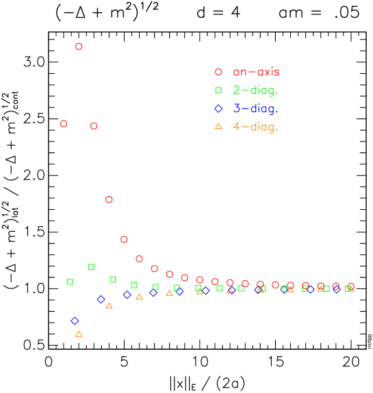
Figure 5: Comparison of the lattice eq. (B.48) and continuum eq. (B.53) results.

B.2 Continuum calculation

Compute the ”generalized propagator” again:

$$\left(m^{2}-\Delta\right)^{-s}(x) = \int_{-\infty}^{\infty}\frac{d^{d}p}{(2\pi)^{d}}\frac{e^{ipx}}{(m^{2}+p^{2})^{s}}$$

$$= \frac{1}{\Gamma(s)}\int_{0}^{\infty}dt\,t^{s-1}\int\frac{d^{d}p}{(2\pi)^{d}}\,e^{ipx-(m^{2}+p^{2})t}$$

$$= \frac{(4\pi)^{-d/2}}{\Gamma(s)}\int_{0}^{\infty}dt\,t^{s-1-d/2}e^{-m^{2}t-x^{2}/(4t)}$$

This time, we end up with modified Bessel functions of the second kind $K_{\nu}$:

$$\int_{0}^{\infty}dt\,t^{s-1-d/2}e^{-m^{2}t-x^{2}/(4t)} = \left(\frac{||x||}{2m}\right)^{s-d/2}\int_{0}^{\infty}du\,u^{s-1-d/2}e^{-m||x||(u+u^{-1})/2}$$

$$= \left(\frac{||x||}{2m}\right)^{s-d/2}2K_{d/2-s}(m||x||)$$

$$\Rightarrow\quad\left(m^{2}-\Delta\right)^{-s}(x) = \frac{(4\pi)^{-d/2}}{\Gamma(s)}\left(\frac{||x||}{2m}\right)^{s-d/2}2K_{d/2-s}(m||x||)$$ (B.51)

The derivation is valid for $x\neq 0$ and $0<\mbox{Re}\,s<d/2$, but analytic continuation to $s=-1/2$ is obvious:

$$\left(m^{2}-\Delta\right)^{1/2}(x) = \frac{(4\pi)^{-d/2}}{\Gamma(-1/2)}\left(\frac{||x||}{2m}\right)^{-(d+1)/2}2K_{(d+1)/2}(m||x||)$$

$$(x\neq 0)$$

In four dimensions, we make use of the fact that Bessel functions with half–integral index are elementary, e.g.

$$K_{5/2}(z) = \left(\frac{\pi}{2z}\right)^{1/2}e^{-z}\left(1+\frac{3}{z}+\frac{3}{z^{2}}\right)$$

$$\Rightarrow\quad\left(m^{2}-\Delta\right)^{1/2}(x) = -\frac{1}{4\pi^{2}}\,\frac{m^{2}}{||x||^{3}}\,e^{-m||x||}\,\left(1+\frac{3}{m||x||}+\frac{3}{m^{2}||x||^{2}}\right)$$ (B.53)

$$= -\frac{3}{4\pi^{2}}\,||x||^{-5}\,e^{-m||x||}\,\left(1+m||x||+m^{2}||x||^{2}/3\right)$$

$$(d=4)$$

B.3 Comparison

The result in eq. (B.53) is the (formal) continuum limit of the lattice expression eq. (B.48). We expect

$$\left(m^{2}-\Delta\right)_{lat}^{1/2}(x) \approx \left(m^{2}-\Delta\right)_{cont}^{1/2}(x)$$

In fact, it has been verified numerically that the lattice expression approaches the continuum result with increasing $||x||/a$, using the Euclidean distance $||x||_{E}$ on the lattice as well. This is shown in Fig. 5 for $am=0.05$.

Appendix C Finite volume effects

When applying the staggered operator $M^{\dagger}M$ hops to neighbors are suppressed by a factor $1/(4(am)^{2}+8)$ with respect to the static mass term. So $aD\xi_{c}(x)$ in eq. (4.27) receives smaller contributions from paths with a larger number of hops connecting $x$ with the source at $y$. As the taxi driver distance $\|x-y\|_{1}$ eq. (4.29) grows, the relative weight of path wrapping around the lattice grows. This growth though is expected to be smaller in comparison on larger lattice sizes $L^{\prime}>L$ simply because the path “around the world” is longer.

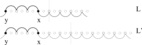
Figure 6: Representation in one dimension of a finite volume effect. The thickness of the lines representing the hops is proportional to the weight of their contribution in eq. (4.27). The vertical dotted lines mark the largest possible taxi driver distance from the source at $y$.

The situation is schematically represented in Fig. 6. Thus we expect

$$\langle f(r)\rangle|_{L}\geq\langle f(r)\rangle|_{L^{\prime}}\,,\quad L^{\prime}>L\,,\quad r>\mbox{some}\;r_{\rm min}\,.$$ (C.54)

This expectation is confirmed by the numerical results shown in Fig. 7, which are obtained at $\beta=6.0\,,\;am=0.01$ comparing $\langle f(r)\rangle$ computed on $L/a=24$ with $L^{\prime}/a=32$ lattices for $0\leq r\leq 2L$. We observe that the minimal distance at which the finite size effects become sizeable is $r_{\rm min}\approx L$. The vertical dotted lines in Fig. 7 correspond to the distances used in eq. (4.33) and eq. (4.34). At these two values of $r$ finite volume effects are absent on the $L/a=24$ lattice.

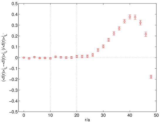
Figure 7: Finite volume effect at $\beta=6.0\,,\;am=0.01$. Comparison of $\langle f(r)\rangle$ computed on $L/a=24$ with $L^{\prime}/a=32$ lattices for $0\leq r\leq 2L$.

The effect leading to eq. (C.54) is the dominant (but not the only one) finite volume effect. It is responsible for the “bumps” of the effective localization range at large distances $r$ visible in Fig. 2, which vanish as the volume increases. The size of this finite volume effect decreases as the mass $am$ increases.

Concluding this section we remark that the maximization operation in the definition of $f(r)$ eq. (4.28) solves the ambiguity for the case when points at the same taxi driver distance but different Euclidean distances from the source are considered. The maximum is presumably attained at the point with the smallest Euclidean distance, which is also the one least affected by the four-dimensional generalization of the finite size effect depicted here in Fig. 6.

References

- [1] K.G. Wilson, New Phenomena In Subnuclear Physics. Part A. Proceedings of the First Half of the 1975 International School of Subnuclear Physics, Erice, Sicily, July 11 - August 1, 1975, ed. A. Zichichi, Plenum Press, New York, 1977, p. 69, CLNS-321.
- [2] J.B. Kogut and L. Susskind, Phys. Rev. D11 (1975) 395.
- [3] L. Susskind, Phys. Rev. D16 (1977) 3031.
- [4] P. Rossi, U. Wolff and D. Zwanziger, Phys. Rev. D30 (1984) 2233.
- [5] H. Kluberg-Stern, A. Morel, O. Napoly and B. Petersson, Nucl. Phys. B190 (1981) 504.
- [6] N. Kawamoto and J. Smit, Nucl. Phys. B192 (1981) 100.
- [7] H. Kluberg-Stern, A. Morel, O. Napoly and B. Petersson, Nucl. Phys. B220 (1983) 447.
- [8] M.F.L. Golterman and J. Smit, Nucl. Phys. B245 (1984) 61.
- [9] G.W. Kilcup and S.R. Sharpe, Nucl. Phys. B283 (1987) 493.
- [10] H. Neuberger, Phys. Lett. B417 (1998) 141, hep-lat/9707022.
- [11] K. Jansen, (2003), hep-lat/0311039.
- [12] D. Toussaint, Nucl. Phys. Proc. Suppl. 106 (2002) 111, hep-lat/0110010.
- [13] C.W. Bernard et al., Phys. Rev. D64 (2001) 054506, hep-lat/0104002.
- [14] BGR, C. Gattringer et al., Nucl. Phys. B677 (2004) 3, hep-lat/0307013.
- [15] CP-PACS, S. Aoki et al., Phys. Rev. D67 (2003) 034503, hep-lat/0206009.
- [16] S. Gottlieb, W. Liu, D. Toussaint, R.L. Renken and R.L. Sugar, Phys. Rev. D35 (1987) 2531.
- [17] H.S. Sharatchandra, H.J. Thun and P. Weisz, Nucl. Phys. B192 (1981) 205.
- [18] C. van den Doel and J. Smit, Nucl. Phys. B228 (1983) 122.
- [19] E. Marinari, G. Parisi and C. Rebbi, Nucl. Phys. B190 (1981) 734.
- [20] HPQCD, C.T.H. Davies et al., Phys. Rev. Lett. 92 (2004) 022001, hep-lat/0304004.
- [21] T. DeGrand, (2003), hep-ph/0312241.
- [22] H. Neuberger, (2004), hep-ph/0402148.
- [23] C.W. Bernard and M.F.L. Golterman, Phys. Rev. D49 (1994) 486, hep-lat/9306005.
- [24] P. Hernandez, K. Jansen and M. Lüscher, Nucl. Phys. B552 (1999) 363, hep-lat/9808010.
- [25] S. Gottlieb, (2003), hep-lat/0310041.
- [26] JLQCD, S. Aoki et al., Comput. Phys. Commun. 155 (2003) 183, hep-lat/0208058.
- [27] R. Frezzotti and K. Jansen, Phys. Lett. B402 (1997) 328, hep-lat/9702016.
- [28] M.A. Clark and A.D. Kennedy, (2003), hep-lat/0309084.
- [29] F. Niedermayer, Nucl. Phys. Proc. Suppl. 73 (1999) 105, hep-lat/9810026.
- [30] O. Martin and S.W. Otto, Phys. Rev. D31 (1985) 435.
- [31] W.H. Press, B.P. Flannery, S.A. Teukolsky and W.T. Vetterling, Numerical Recipes: The Art of Scientific Computing, 2nd ed. (Cambridge University Press, Cambridge (UK) and New York, 1992).
- [32] R.A. Horn and C.R. Johnson, Matrix Analysis (Cambridge University Press, Cambridge (UK) and New York, 1985).
- [33] T. Kalkreuter, Phys. Rev. D51 (1995) 1305, hep-lat/9408013.
- [34] S. Kim and D.K. Sinclair, Phys. Rev. D52 (1995) 2614, hep-lat/9502004.
- [35] R. Gupta, G. Guralnik, G.W. Kilcup and S.R. Sharpe, Phys. Rev. D43 (1991) 2003.
- [36] S. Kim and S. Ohta, Phys. Rev. D61 (2000) 074506, hep-lat/9912001.
- [37] R. Sommer, Nucl. Phys. B411 (1994) 839, hep-lat/9310022.
- [38] ALPHA, M. Guagnelli, R. Sommer and H. Wittig, Nucl. Phys. B535 (1998) 389, hep-lat/9806005.
- [39] ALPHA, U. Wolff, Comput. Phys. Commun. 156 (2004) 143, hep-lat/0306017.
- [40] A. Hasenfratz and F. Knechtli, Phys. Rev. D64 (2001) 034504, hep-lat/0103029.
- [41] A. Erdélyi ed., Higher Transcendental Functions, Vol. II (Robert E. Krieger Publishing Company, Malabar, Florida, 1981).
- [42] B. Bunk, Nucl. Phys. Proc. Suppl. B63 (1998) 952, hep-lat/9805030.