CERN-PH-TH/2004-029

Critical slowing down of topological modes

Luigi Del Debbio,^a Gian Mario Manca,^b Ettore Vicari$\,{}^{b}$

^a CERN, Department of Physics, TH Division, CH-1211 Geneva 23

^b Dipartimento di Fisica dell’Università di Pisa, Pisa, Italy

We investigate the critical slowing down of the topological modes using local updating algorithms in lattice 2-$d$ $\mathrm{CP}^{N-1}$ models. We show that the topological modes experience a critical slowing down that is much more severe than the one of the quasi-Gaussian modes relevant to the magnetic susceptibility, which is characterized by $\tau_{\rm mag}\sim\xi^{z}$ with $z\approx 2$. We argue that this may be a general feature of Monte Carlo simulations of lattice theories with non-trivial topological properties, such as QCD, as also suggested by recent Monte Carlo simulations of 4-$d$ SU($N$) lattice gauge theories.

Monte Carlo simulations of critical phenomena in statistical mechanics and of quantum field theories, such as QCD, in the continuum limit are hampered by the problem of critical slowing down (CSD) [1]. The autocorrelation time $\tau$, which is related to the number of iterations needed to generate a new independent configuration, grows with increasing length scale $\xi$. In simulations of lattice QCD where the upgrading methods are essentially local, it has been observed that the autocorrelation times of topological modes are typically much larger than those of other observables not related to topology, such as Wilson loops and their correlators, see for instance Refs. [2]–[7]. Recent Monte Carlo simulations [5, 6] of the 4-$d$ SU($N$) lattice gauge theories (for $N=3,4,6$) provided evidence of a severe CSD for the topological modes, using a rather standard local overrelaxed upgrading algorithm (constructed taking a mixture of overrelaxed microcanonical and heat-bath updatings). Indeed, the autocorrelation time $\tau_{Q}$ of the topological charge grows very rapidly with the length scale $\xi\equiv\sigma^{-1/2}$, where $\sigma$ is the string tension, showing an apparent exponential behavior $\tau_{Q}\sim\exp(c\xi)$ in the range of values of $\xi$ where data are available. This peculiar effect was not observed in plaquette–plaquette or Polyakov line correlations, suggesting an approximate decoupling between topological modes and non-topological ones, such as those determining the confining properties. The issue of the CSD of topological modes is particularly important for lattice QCD, because it may pose a serious limitation for numerical studies of physical issues related to topological properties, such as the mass and the matrix elements of the $\eta^{\prime}$ meson, and in general the physics related to the broken U(1)_A symmetry.

The above-mentioned results suggest that the dynamics of the topological modes in Monte Carlo simulations is rather different from that of quasi-Gaussian modes. CSD of quasi-Gaussian modes for traditional local algorithms, such as standard Metropolis or heat bath, is related to an approximate random-walk spread of information around the lattice. Thus, the corresponding autocorrelation time $\tau$ is expected to behave as $\tau\sim\xi^{2}$ (an independent configuration is obtained when the information travels a distance of the order of the correlation length $\xi$, and the information is transmitted from a given site/link to the nearest neighbors). This guess is correct for Gaussian (free-field) models; in general it is expected that $\tau\sim\xi^{z}$, where $z$ is a dynamical critical exponent, and $z\approx 2$ for quasi-Gaussian modes.  On the other hand, in the presence of relevant topological modes, the random-walk picture may fail, and therefore we may have qualitatively different types of CSD. These modes could give rise to sizeable free-energy barriers separating different regions of the configuration space. The evolution in this space would then present a long-time relaxation due to transitions between different topological charge sectors, and the corresponding autocorrelation time should behave as $\tau_{\rm top}\sim\exp F_{b}$, where $F_{b}$ is the typical free-energy barrier between different topological sectors. However, for this picture to become more quantitative, one should understand how the typical free-energy barriers scale with the correlation length. For example, we may still have a power-law behavior if $F_{b}\sim\ln\xi$, or an exponential behavior if $F_{b}\sim\xi^{\theta}$. It is worth mentioning that in physical systems, such as random-field Ising systems [9] and glass models [10], the presence of significant free-energy barriers in the configuration space causes a very slow dynamics, and an effective separation of short-time relaxation within the free-energy basins from long-time relaxation related to the transitions between basins. In the case of random-field Ising systems the free-energy barrier picture supplemented with scaling arguments leads to the prediction that $\tau\sim\exp(c\xi^{\theta})$, where $\theta$ is a universal critical exponent [11].

Motivated by the recent results of Ref. [5], suggesting an exponential CSD for the topological modes in 4-$d$ SU($N$) lattice gauge theories, we decided to investigate this issue in 2-d $\mathrm{CP}^{N-1}$ models [12, 13], where we can study in detail the dependence of the autocorrelation time on the length scale $\xi$ as $N$ is varied. Since the 2-d $\mathrm{CP}^{N-1}$ models possess interesting properties expected to hold in QCD, such as asymptotic freedom and a non-trivial topological structure, they have often been used as a theoretical laboratory. In particular, their lattice formulation has been considered to check and develop methods to investigate topological properties in asymptotically free models, exploiting also large-$N$ analytic calculations. See, e.g., Refs. [14]–[26]. The CSD of the topological modes in lattice $\mathrm{CP}^{N-1}$ models, and in particular the behavior of the autocorrelation time of the topological susceptibility, has already been discussed in Refs. [18, 19], where the hypothesis of a strong CSD was put forward on the basis of a few rough estimates of $\tau_{\rm top}$ for the $\mathrm{CP}^{9}$ model, and the fact that for large $N$, $N=O(100)$ say, it was not possible to correctly sample the topological sectors. In this paper we present high-statistics Monte Carlo simulations using local updating algorithms, such as Metropolis and overrelaxed algorithms, obtaining rather accurate estimates of the topological susceptibility and its integrated autocorrelation time. The results provide a definite evidence that, under local updating algorithms, the CSD experienced by the topological modes turns out to be much more severe than the CSD of the magnetic susceptibility, whose autocorrelation time shows a power-law behavior $\tau_{\rm mag}\sim\xi^{z}$ with $z\approx 2$.

Two-dimensional $\mathrm{CP}^{N-1}$ models are defined by the action

$$S={N\over g}\int d^{2}x\,\overline{D_{\mu}z}D_{\mu}z,$$ (1)

where $z$ is an $N$-component complex scalar field subject to the constraint $\bar{z}z=1$, and the covariant derivative $D_{\mu}=\partial_{\mu}+iA_{\mu}$ is defined in terms of the composite field $A_{\mu}=i\bar{z}\partial_{\mu}z$. Like QCD, they are asymptotically free and present non-trivial topological structures (instantons, anomalies, $\theta$ vacua). The large-$N$ expansion is performed by keeping the coupling $g$ fixed [12, 13]. A topological charge density operator $q(x)$ can be defined as

$$q(x)={1\over 2\pi}\epsilon_{\mu\nu}\partial_{\mu}A_{\nu},$$ (2)

with the related topological susceptibility

$$\chi_{t}=\int d^{2}x\langle q(x)q(0)\rangle.$$ (3)

We consider the lattice formulation [27, 28, 29, 18]

$$S_{L} = -N\beta\Bigl{[}{4\over 3}\sum_{n,\mu}\left(\bar{z}_{n+\mu}z_{n}\lambda_{n,\mu}+\bar{z}_{n}z_{n+\mu}\bar{\lambda}_{n,\mu}-2\right)$$

$$-{1\over 12}\sum_{n,\mu}\left(\bar{z}_{n+2\mu}z_{n}\lambda_{n,\mu}\lambda_{n+\mu,\mu}+\bar{z}_{n}z_{n+2\mu}\bar{\lambda}_{n,\mu}\bar{\lambda}_{n+\mu,\mu}-2\right)\Bigr{]},$$

where, beside the complex $N$-component vector $z$ satisfying $\bar{z}z=1$, the complex variable $\lambda_{n,\mu}$ has been introduced, which satisfies $\bar{\lambda}_{n,\mu}\lambda_{n,\mu}=1$; $S_{L}$ is a tree-order Symanzik-improved lattice action [30, 18]. The correlation function is defined as

$$G(x)=\langle{\rm Tr}P(x)P(0)\rangle_{\rm conn},$$ (5)

where $P=\bar{z}\otimes z$. One can define the magnetic susceptibility $\chi_{m}$ and the second-moment correlation length $\xi$ from its small-momentum behavior:

$$\chi_{m}=\widetilde{G}(0),\quad\xi^{2}={1\over 4\sin^{2}(q_{\rm m}/2)}{\widetilde{G}(0)-\widetilde{G}(q_{\rm m})\over\widetilde{G}(q_{\rm m})},$$ (6)

where $q_{\rm m}=(2\pi/L,0)$ is the minimum non-zero momentum on a lattice of size $L$ with periodic boundary conditions (see Ref. [31] for a discussion of this estimator of the second-moment correlation length). We consider the geometrical definition of lattice topological charge proposed in Ref. [29], which meets the demands that the topological charge on the lattice have the classical correct continuum limit and be an integer for every lattice configuration in a finite volume with periodic boundary conditions. As a result both the topological charge and its susceptibility do not require lattice renormalizations. It is given by [29]

$$Q=\sum_{n}{1\over 2\pi}{\rm Im}\left[\ln{\rm Tr}(P_{n+\mu+\nu}P_{n+\mu}P_{n})+\ln{\rm Tr}(P_{n+\nu}P_{n+\mu+\nu}P_{n})\right],\qquad\mu\neq\nu,$$ (7)

where the imaginary part of the logarithm is to be taken in $(-\pi,\pi)$. As shown in Refs. [18, 21], this definition is effective for sufficiently large values of $N$, where unphysical dislocations [32] should not affect the continuum limit of its matrix elements. The corresponding topological susceptibility is obtained by

$$\chi_{t}={1\over V}\langle Q^{2}\rangle,$$ (8)

where $V$ is the volume of the lattice.

The autocorrelation function $C_{O}(t)$ ($t$ is the discrete Monte Carlo time, where a time unit is given by a sweep, i.e. an update of all lattice variables) of a given quantity $O$ is defined as

$$C_{O}(t)=\left\langle\left(O(t)-\langle O\rangle\right)\left(O(0)-\langle O\rangle\right)\right\rangle,$$ (9)

where the averages are taken at equilibrium. The integrated autocorrelation time $\tau_{O}$ associated with $O$ is given by

$$\tau_{O}={1\over 2}\sum_{t=-\infty}^{t=+\infty}{C_{O}(t)\over C_{O}(0)}.$$ (10)

Estimates of $\tau_{O}$ can be obtained by the binning method (see e.g. Ref. [33] for a discussion of this method and its systematic errors), using the estimator

$$\tau_{O}={E^{2}\over 2E_{0}^{2}},$$ (11)

where $E_{0}$ is the naive error calculated without taking into account the autocorrelations, and $E$ is the error found after binning, i.e. when the error estimate becomes stable with respect to increasing the block size $n_{b}$. The statistical error $\Delta\tau_{O}$ is just given by $\Delta\tau_{O}/\tau_{O}=\sqrt{2/n_{b}}$, where $n_{b}$ is the number of blocks corresponding to the estimate of $E$. As discussed in Ref. [33] this procedure leads to a systematic error of $O(\tau_{O}/b)$, where $b$ is the size of the blocks. In our cases the ratio $\tau_{O}/b$ will always be much smaller than the statistical error, so we will neglect it. Equation (11) can be easily extended to the case where the quantity $O$ is measured every $n_{m}$ sweeps, i.e. $\tau_{O}=n_{m}E^{2}/(2E_{0}^{2})$, which is of course meaningful only if $n_{m}\ll\tau_{O}$.

We performed Monte Carlo simulations for $N=10,15,21$, for which the geometrical definition (7) should be effective to describe the topological modes relevant to the continuum limit. We measured the magnetic susceptibility $\chi_{m}$, the correlation length $\xi$, the topological susceptibility $\chi_{t}$, and the integrated autocorrelation times of $\chi_{m}$ and $\chi_{t}$, respectively $\tau_{\rm mag}$ and $\tau_{\rm top}$. We considered two types of updating methods: a standard Metropolis and a mixed method containing overrelaxation procedures. A summary of our runs is reported in Table 1. Finite-size effects in lattice $\mathrm{CP}^{N-1}$ models are rather large and peculiar, especially at large $N$ [34]. We performed our simulations for lattice size $L$ sufficiently large to guarantee that finite-size effects were at most $O(10^{-3})$ for $\xi$ and smaller than 1% for $\chi_{t}$, i.e. $L/\xi\mathrel{\hbox to0.0pt{\lower 3.0pt\hbox{$\mathchar 536\relax$}\hss}\raise 2.0pt\hbox{$\mathchar 318\relax$}}10$ for $N=10$, $L/\xi\mathrel{\hbox to0.0pt{\lower 3.0pt\hbox{$\mathchar 536\relax$}\hss}\raise 2.0pt\hbox{$\mathchar 318\relax$}}13$ for $N=15$, and $L/\xi\mathrel{\hbox to0.0pt{\lower 3.0pt\hbox{$\mathchar 536\relax$}\hss}\raise 2.0pt\hbox{$\mathchar 318\relax$}}15$ for $N=21$. Each run consisted typically of a few million sweeps for the smallest values of $\beta$, increasing up to approximately 50 million for the largest $\beta$’s.

Table 1: Summary of the Monte Carlo data. The Metropolis and the mixed overrelaxed upgrading methods are indicated by mt and ov respectively.

$N$	$\beta$	$L$	upgrade	$\xi$	$\chi_{t}\xi^{2}$	$\tau_{\rm top}$
10	0.59	20	mt	1.854(8)	0.02223(24)	17.7(6)
	0.61	24	mt	2.113(6)	0.02181(19)	31.1(1.0)
	0.61	24	ov	2.118(3)	0.02204(11)	3.44(10)
	0.63	30	mt	2.410(5)	0.02145(10)	53.3(1.9)
	0.63	30	ov	2.409(3)	0.02117(14)	5.6(3)
	0.65	32	mt	2.748(5)	0.02048(10)	83(3)
	0.65	32	ov	2.7471(12)	0.02064(6)	7.8(2)
	0.65	36	mt	2.750(5)	0.02061(11)	85(3)
	0.67	36	mt	3.128(6)	0.01986(12)	150(5)
	0.67	36	ov	3.127(2)	0.01993(7)	12.7(3)
	0.70	45	mt	3.787(6)	0.01911(13)	367(17)
	0.70	30	ov	3.898(2)	0.01926(7)	26.9(4)
	0.70	40	ov	3.795(2)	0.01906(6)	27.3(8)
	0.70	45	ov	3.7885(10)	0.01914(5)	26.7(4)
	0.70	50	ov	3.790(2)	0.01916(7)	27.1(1.1)
	0.72	54	ov	4.304(2)	0.01875(6)	44.3(1.6)
	0.75	60	mt	5.201(10)	0.01851(20)	1550(150)
	0.75	60	ov	5.195(3)	0.01815(8)	98(4)
	0.75	66	ov	5.198(4)	0.01821(16)	99(3)
	0.75	72	ov	5.199(3)	0.01836(12)	99(5)
	0.80	80	ov	7.091(3)	0.01757(12)	420(20)
	0.80	90	ov	7.087(6)	0.01772(22)	435(40)
	0.80	100	ov	7.090(6)	0.01752(24)	394(20)
	0.85	120	ov	9.651(5)	0.01729(24)	1900(100)
	0.85	140	ov	9.653(11)	0.0180(5)	1900(200)
	0.87	150	ov	10.904(10)	0.0177(5)	4800(700)
15	0.54	25	ov	1.7013(7)	0.01382(4)	6.4(2)
	0.56	30	ov	1.9409(9)	0.01322(5)	10.9(3)
	0.58	36	ov	2.2126(9)	0.01266(5)	19.5(4)
	0.60	42	ov	2.5185(12)	0.01221(7)	35.7(7)
	0.63	45	ov	3.050(3)	0.01180(14)	90(6)
	0.63	50	ov	3.058(3)	0.01191(10)	89(6)
	0.65	45	ov	3.462(3)	0.01128(11)	193(5)
	0.65	54	ov	3.4630(11)	0.01150(7)	198(9)
	0.67	60	ov	3.9269(14)	0.01135(5)	400(20)
	0.70	75	ov	4.735(3)	0.01137(16)	1330(80)
	0.72	85	ov	5.361(3)	0.01158(25)	3100(300)
	0.73	90	ov	5.705(3)	0.01132(20)	5400(600)
21	0.49	24	ov	1.4203(5)	0.00953(3)	10.6(2)
	0.51	28	ov	1.6208(4)	0.00900(3)	20.4(4)
	0.54	30	ov	1.9700(6)	0.00845(4)	61.0(1.4)
	0.54	36	ov	1.9715(6)	0.00843(5)	60.4(1.9)
	0.57	30	ov	2.3887(8)	0.00809(7)	204(9)
	0.57	38	ov	2.3893(9)	0.00802(7)	200(6)
	0.57	42	ov	2.3895(9)	0.00800(7)	201(9)
	0.60	45	ov	2.8850(9)	0.00807(8)	820(30)
	0.60	48	ov	2.8884(6)	0.00776(8)	770(30)
	0.60	50	ov	2.888(2)	0.00796(10)	740(40)
	0.62	54	ov	3.275(2)	0.00777(15)	2160(150)
	0.62	56	ov	3.278(2)	0.00789(10)	1980(130)
	0.62	60	ov	3.277(2)	0.00807(22)	1900(200)
	0.64	60	ov	3.712(2)	0.00800(14)	5670(220)
	0.64	64	ov	3.709(2)	0.00798(16)	6100(250)
	0.66	72	ov	4.209(2)	0.00807(25)	19000(3000)

Let us first consider the results of the standard Metropolis algorithm (50% acceptance, 10 hits per lattice variable). Figure 1 shows the results for the integrated autocorrelation times of the magnetic and topological susceptibilities obtained for the $\mathrm{CP}^{9}$ model. The autocorrelation time $\tau_{\rm mag}$ of $\chi_{m}$ is in agreement with the expected power-law behavior, i.e. $\tau_{\rm mag}=c\xi^{z}$ with $z$ slightly larger than 2 (a fit of all data to $\tau_{\rm mag}=c\xi^{z}$ gives $z=2.30(5)$ with $\chi^{2}/{\rm d.o.f.}\simeq 0.9$). On the other hand, the autocorrelation time $\tau_{\rm top}$ of $\chi_{t}$ appears to increase much faster. In particular, a power-law behavior with $z\approx 2$ can be definitely excluded. The data for the largest available $\xi$ suggest larger values of $z$, i.e. $z\mathrel{\hbox to0.0pt{\lower 3.0pt\hbox{$\mathchar 536\relax$}\hss}\raise 2.0pt\hbox{$\mathchar 318\relax$}}4$. Moreover, an exponential ansatz $\tau_{\rm top}\sim\exp(c\xi^{\theta})$ turns out to be well fitted by all data, with $\theta\approx 0.3$, as shown in Fig. 1.

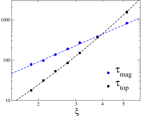
Figure 1: Integrated autocorrelation time of the magnetic susceptibility and the topological susceptibility for the $\mathrm{CP}^{9}$ model and Metropolis updating. The lines are the results of the fits described in the text, power-law and exponential fits for $\tau_{\rm mag}$ and $\tau_{\rm top}$ respectively.

However, in order to obtain a more precise characterization of the topological CSD, data for larger values of $\xi$ are necessary, and this becomes rather expensive when using a standard Metropolis algorithm. A substantial improvement is obtained by using a more effective local updating algorithm, constructed by employing also overrelation procedures. At each site the upgrading method was chosen stochastically between an overrelaxed microcanonical (80%), an over-heat bath [35] (16%), and the Metropolis algorithm (4%) to ensure ergodicity. Some details on the application of the above algorithms to lattice $\mathrm{CP}^{N-1}$ models can be found in Ref. [18]. Similar mixtures are usually employed to obtain effective local updating algorithms for 4-$d$ SU($N$) gauge theories. The above mixed algorithm turns out to be much more effective than the standard Metropolis. For example for $N=10$ and $\beta=0.70$ ($\xi=3.8$), we found $\tau_{\rm mag}\approx 380$ and $\tau_{\rm top}\approx 367$ using the Metropolis algorithm, and $\tau_{\rm mag}\approx 7$ and $\tau_{\rm top}\approx 27$ using the above overrelaxed updating. In addition, the mixed algorithm requires less computer time by approximately a factor 2. This allowed us to obtain reliable estimates of $\tau_{\rm top}$ up to $\xi\simeq 10$ for $N=10$ with a reasonable amount of computer time. Actually, we do not exclude that a further improvement can be achieved by optimizing the mixture, since we did not really perform a detailed study of this issue.  Moreover, we performed simulations for larger values of $N$, $N=15$ and $N=21$, which will be useful to understand the behavior of $\tau_{\rm top}$, and to compare $\chi_{t}$ with the available large-$N$ results. The results are reported in Table 1.

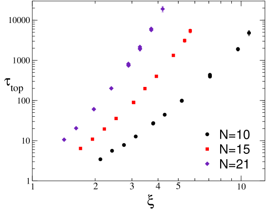
Figure 2: Log-log plot of the integrated autocorrelation time $\tau_{\rm top}$ versus $\xi$, for the $\mathrm{CP}^{9}$, $\mathrm{CP}^{14}$ and $\mathrm{CP}^{20}$ models, obtained using the mixed overrelaxed algorithm described in the text.

Using the above random mixture of algorithms, the quasi-Gaussian modes are expected to be still characterized by power-law CSD with $z\approx 2$. This is substantially confirmed by our simulations. The data for the autocorrelation time $\tau_{\rm top}$ of $\chi_{t}$ are shown in Fig. 2. It is already apparent from the log-log plot of $\tau_{\rm top}$ versus $\xi$ that the data do not agree with a simple power law, i.e. with $\tau_{\rm top}\approx c\xi^{z}$, on the whole range of $\xi$ explored by this work. Moreover, even assuming an asymptotic power-law behavior that sets at relatively large $\xi$, values $z\approx 2$ can be definitely excluded, but substantially larger $z$ are suggested by the data for the largest $\xi$. In the case of $N=10$ the behavior of $\tau_{\rm top}$ looks qualitatively similar to the one found using the Metropolis algorithm.

Comparing the data of $\tau_{\rm top}$ at different $N$ but fixed $\xi$, we note that the quantity $N^{-1}\log_{10}\tau_{\rm top}$ seems to converge to a non-trivial large-$N$ limit, the approach being roughly $O(1/N)$, see also Fig. 3. This fact is also suggested by the following simple picture. Let us assume that the transition from one topological sector to the other happens by tunnelling through a potential barrier. The resulting autocorrelation time is $\tau\sim\exp S_{b}$ (neglecting entropy), where $S_{b}$ is the action of the typical configurations that are at the boundary of the different topological sectors. Let us also assume that these configurations are instanton-like. Since the instanton action is given by $S_{I}=N2\pi/g(\rho)$ [37] where $\rho$ is the size of the instanton and $g(\rho)$ the running coupling at scale $\rho$, we should expect that $\ln\tau_{\rm top}=O(N)$. Note that the same arguments apply to 4-$d$ SU($N$) lattice gauge theories, and the estimates of the topological autocorrelation times for $N=3,4,6$ [5, 4] are indeed consistent with the above dependence.

Proceeding further within this instanton picture, one arrives at a power-law behavior with $z\sim N$. Let us further assume that the size of the relevant instanton configurations at the boundary of different topological sectors is given by $\rho\approx a$ (see, e.g., Refs. [4, 36]). Then, we should have $g(a)\sim 1/\beta$ and using asymptotic freedom $\xi\sim\exp(2\pi\beta)$, thus $\tau_{\rm top}\sim\exp S_{I}\sim\xi^{z}$ with $z\sim N$. As is already apparent from Fig. 2, a reasonable fit to a simple power law

$$\tau_{\rm top}=b_{N}\xi^{c_{N}N}$$ (12)

can be obtained only by discarding several data points at the smallest values of $\xi$. As Fig. 2 already shows, the fitted value of $c_{N}$ tends to increase when more and more data at small $\xi$ are discarded. We can tentatively determine lowest bounds for the power coefficient $c_{N}$ by using only the largest values of $\xi$. For $N=10$, using the data for the last three $\beta$-values, i.e. data for $\xi\mathrel{\hbox to0.0pt{\lower 3.0pt\hbox{$\mathchar 536\relax$}\hss}\raise 2.0pt\hbox{$\mathchar 318\relax$}}7$, we obtain $c_{10}=0.51(2)$, $b_{10}=0.02(1)$. In this case, we also note that there is a hint of stability in the results for $c_{10}$, because a consistent value is already obtained taking data for $\xi>5$, with an acceptable $\chi^{2}$. In the case $N=15$, the last three $\beta$-values give $c_{15}=0.49(4)$, $b_{15}=0.02(2)$. Finally, for $N=21$ the data for the last three $\beta$-values give $c_{21}=0.41(2)$, $b_{21}=0.07(4)$. We note that these results for $c_{N}$ are rather close, consistently with the expectation that $c_{N}=O(1)$ in the large-$N$ limit. Consistent results are obtained by considering a more general ansatz such as $\tau_{\rm top}=a_{N}+b_{N}\xi^{c_{N}N}$, where we also allow for a constant term. Note that the naive guess obtained simply by assuming $g(\rho=a)=1/\beta$ would be $z=N$. In conclusion, assuming a power-law CSD, this analysis indicates that $z\mathrel{\hbox to0.0pt{\lower 3.0pt\hbox{$\mathchar 536\relax$}\hss}\raise 2.0pt\hbox{$\mathchar 318\relax$}}N/2$.

On the other hand, Fig. 3 is also suggestive of an exponential behavior, which emerges naturally from tunnelling through a free-energy barrier whose size scales like $\xi^{\theta}$. Such exponential behavior gives a good description of the data in the whole range of $\xi$ explored by this work. Therefore, we also consider an exponential ansatz

$${1\over N}\log_{10}\tau_{\rm top}=a_{N}+b_{N}\xi^{\theta_{N}},$$ (13)

where $a_{N}$, $b_{N}$ and $\theta_{N}$ are $O(1)$ in the large-$N$ limit, and $\theta_{N}\approx 1/2$. We may further simplify this ansatz by assuming that $\theta_{N}$ is independent of $N$, i.e. $\theta_{N}=\theta$. A global fit to the data gives $\theta=0.49(2)$. This result was obtained by discarding a few data points at the smallest $\xi$ for each $N$, i.e. taking the data for $\xi\mathrel{\hbox to0.0pt{\lower 3.0pt\hbox{$\mathchar 536\relax$}\hss}\raise 2.0pt\hbox{$\mathchar 318\relax$}}3$ ($\beta\geq 0.70$) at $N=10$, $\xi\mathrel{\hbox to0.0pt{\lower 3.0pt\hbox{$\mathchar 536\relax$}\hss}\raise 2.0pt\hbox{$\mathchar 318\relax$}}2$ at $N=15$ and $N=21$ (corresponding to $\beta\geq 0.56$ and $\beta\geq 0.54$ respectively), in order to obtain an acceptable $\chi^{2}/{\rm d.o.f.}\approx 0.9$. In Fig. 3 we also show the curve obtained by fits with $\theta=1/2$, for which, using the same data as in the above global fit, we obtained $a_{10}=-0.174(3)$ and $b_{10}=0.163(2)$ with $\chi^{2}/{\rm d.o.f.}\approx 1.1$, $a_{15}=-0.179(3)$ and $b_{15}=0.178(2)$ with $\chi^{2}/{\rm d.o.f.}\approx 0.4$, $a_{21}=-0.169(2)$ and $b_{21}=0.181(2)$ with $\chi^{2}/{\rm d.o.f.}\approx 1.0$.

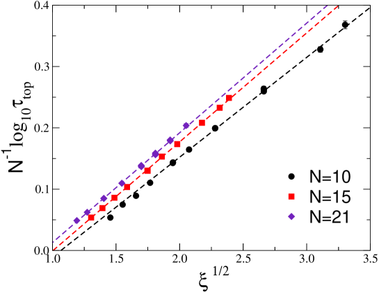
Figure 3: The quantity $N^{-1}\log_{10}\tau_{\rm top}$ versus $\xi^{-1/2}$. The lines show the results of the exponential fits $\tau_{\rm top}\sim\exp(b_{N}\xi^{\theta})$ with $\theta=1/2$; see text.

In conclusion, the CSD of the topological modes in Monte Carlo simulation employing local updating algorithms turns out to be much stronger than the one experienced by quasi-Gaussian modes. This has been inferred by comparing the integrated autocorrelation time of the magnetic and topological susceptibilities as a function of $\xi$. Their behavior suggests an effective separation of short-time relaxation within the topological sectors from long-time relaxation related to the transitions between different topological sectors. A heuristic explanation can be devised by assuming the presence of significant free-energy barriers in the configuration space between different topological sectors, with the system changing topology by tunnelling through such barriers. An exponential ansatz, i.e. $\tau_{\rm top}\sim\exp(c\xi^{\theta})$ with $\theta\approx 1/2$, provides a good effective description of the data in the range of $\xi$ where data are available. However, the statistical analysis of the available data for $\tau_{\rm top}$ does not actually allow us to distinguish between an exponential CSD and an asymptotic power-law behavior with $z\mathrel{\hbox to0.0pt{\lower 3.0pt\hbox{$\mathchar 536\relax$}\hss}\raise 2.0pt\hbox{$\mathchar 318\relax$}}N/2$ setting at relatively large $\xi$. Power-law behaviors with smaller exponents can definitely be excluded by our analysis. Data for larger $\xi$ and/or a better modellization of the Monte Carlo dynamics of the topological modes would be needed to further clarify this issue. We argue that the severe CSD experienced by the topological modes under local updating algorithms should be a general feature of Monte Carlo simulations of lattice models with non-trivial topological properties, since the mechanism behind this phenomenon should be similar. This is also supported by recent Monte Carlo simulations of 4-$d$ lattice SU($N$) gauge theories reported in Refs. [5, 4]. Indeed, the estimates of autocorrelation time $\tau_{Q}$ of the topological charge  recently reported in Ref. [5] (measured using the cooling technique) showed a rapid increase with the length scale, and an apparent exponential behavior $\tau_{Q}\sim\exp(c\xi)$ in the range of values of $\xi$ where data were available, for all $N=3,4,6$. We stress again that the CSD of topological modes may represent a serious limitation for simulations of lattice QCD, in order to study physical issues determined by the topological excitations, such as the physics of the $\eta^{\prime}$ meson. Our results suggest that the contribution of the correlation time to the total cost of a simulation could be higher than is usually assumed, if one wants to sample the different topological sectors correctly. In particular, it may worsen the current cost estimates of the dynamical fermion simulations for lattice QCD, see e.g. Ref. [38], where it is usually assumed that the autocorrelation time only contributes a factor of $\xi$.

An interesting question would be whether other, possibly non-local, updating algorithms may eliminate or at least improve the severe form of CSD of topological modes. Cluster algorithms turn out not to be effective in $\mathrm{CP}^{N-1}$ models [17, 40]. Instead, as shown in Ref. [39], multigrid Monte Carlo algorithms achieve a substantial reduction of the CSD of the quasi-Gaussian modes relevant to the magnetic susceptibility. It is however not clear if they can also accelerate the decorrelation of the topological modes. Let us mention here that algorithms based on the simulated tempering method [41] were also tried in Ref. [19], but apparently without achieving a particular advantage.

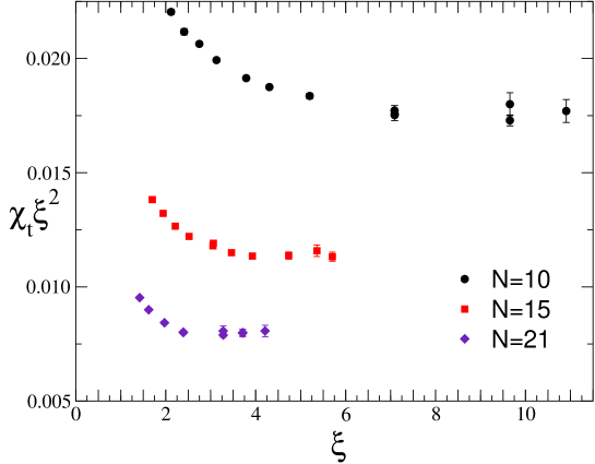
Figure 4: $\chi_{t}\xi^{2}$ versus $\xi$ for $N=10,15,21$.

Finally let us discuss the results for the topological susceptibility; data for the dimensionless quantity $\chi_{t}\xi^{2}$, reported in Fig. 4, clearly show a plateau for the largest values of $\xi$, where one can extract an estimate of the continuum limit of $\chi_{t}\xi^{2}$. We obtain:

$$\chi_{t}\xi^{2}=0.0175(3)\quad{\rm for}\quad N=10,$$ (14)

$$\chi_{t}\xi^{2}=0.0113(2)\quad{\rm for}\quad N=15,$$

$$\chi_{t}\xi^{2}=0.0080(2)\quad{\rm for}\quad N=21,$$

where, prudently, we have taken the typical error on the data at the plateau as estimate of the uncertainty. Compatible but substantially less precise results for $N=10,21$ are reported in Refs. [18, 19]. The estimates (14) may be compared with the available results obtained in the framework of the large-$N$ expansion [42]:

$$\chi_{t}\xi^{2}={1\over 2\pi N}-{0.060\over N^{2}}+O(1/N^{3}).$$ (15)

We note that the estimates (14) are slightly larger. Actually they suggest a $O(1/N^{2})$ contribution given by $c_{2}/N^{2}$ with $c_{2}\simeq 0.2$. Indeed, by evaluating the quantity $N^{2}(\chi_{t}\xi^{2}-{\textstyle\frac{1}{2\pi N}})$, using the estimates (14), one would obtain $c_{2}=0.16(3)$ for $N=10$, $c_{2}=0.16(4)$ for $N=15$, and $c_{2}=0.19(9)$ for $N=21$. However, this apparent discrepancy can be easily accounted for by a slow approach to the large-$N$ regime, and the apparent stability of the $O(1/N^{2})$ correction may be only a chance. This point deserves further investigation.

Acknowledgements We thank Maurizio Davini for his valuable and indispensable technical support. We also thank Philippe de Forcrand, Martin Lüscher, Andrea Pelissetto, and Paolo Rossi for interesting and useful discussions.

References

- [1] For a general introduction to critical slowing down in Monte Carlo simulations, see, e.g., A. D. Sokal, in Quantum Fields on the Computer, ed. M. Creutz (World Scientific, Singapore, 1992).
- [2] B. Alles, G. Boyd, M. D’Elia, A. Di Giacomo, and E. Vicari, Phys. Lett. B 389 (1996) 107.
- [3] P. de Forcrand, M.G. Perez, J.E. Hetrick, and I. Stamatescu, Nucl. Phys. (Proc. Suppl.) 63 (1998) 549, [hep-lat/9710001].
- [4] B. Lucini and M. Teper, JHEP 06 (2001) 050.
- [5] L. Del Debbio, H. Panagopoulos, and E. Vicari, JHEP 08 (2002) 044.
- [6] L. Del Debbio, H. Panagopoulos, P. Rossi, and E. Vicari, Phys. Rev. D 65 (2002) 021501(R); JHEP 01 (2002) 009.
- [7] D. B. Leinweber, A. G. Williams, J. B. Zhang and F. X. Lee, arXiv:hep-lat/0312035.
- [8] S. Adler, Phys. Rev. D 37 (1988) 458.
- [9] A.T. Nattermann, in: A.P. Young (Ed.), Spin Glasses and Random Fields, World Scientific, Singapore, 1998, [cond-mat/9705295].
- [10] J. Bouchaud, L. F. Cugliandolo, J. Kurchan, M. Mezard, A.P. Yound (Ed.). Spin Glasses and Random Fields, World Scientific, Singapore, 1998, [cond-mat/9702070]
- [11] D.S. Fisher, Phys. Rev. Lett. 56 (1986) 416.
- [12] A. D’Adda, P. Di Vecchia, and M. Lüscher, Nucl. Phys. B 146 (1979) 63.
- [13] E. Witten, Nucl. Phys. B 149 (1979) 285.
- [14] M. Campostrini and P. Rossi, Riv. Nuovo Cimento 16, n.6, (1993) 1.
- [15] N. Seiberg, Phys. Rev. Lett. 53 (1984) 637.
- [16] U. Wolff, Phys. Lett. B 284 (1992) 94.
- [17] K. Jansen and U.J. Wiese, Nucl. Phys. B 370 (1992) 762.
- [18] M. Campostrini, P. Rossi, and E. Vicari, Phys. Rev. D 46 (1992) 2647 and 4643.
- [19] E. Vicari, Phys. Lett. B 309 (1993) 139.
- [20] R. Burkhalter, Phys. Rev. D 54 (1996) 4121.
- [21] L. Rastelli, P. Rossi, and E. Vicari, Nucl. Phys. B 489 (1997) 453.
- [22] J.C. Plefka and S. Samuel, Phys. Rev. D 56 (1997) 44.
- [23] E. Vicari, Nucl. Phys. B 554 (1999) 301.
- [24] B. Alles, L. Cosmai, M. D’Elia, and A. Papa, Phys. Rev. D 62 (2000) 094507.
- [25] R. Burkhalter, M. Imachi, Y. Shinno, and H. Yoneyama, Prog. Theor. Phys. 106 (2001) 613.
- [26] V. Azcoiti, G. Di Carlo, A. Galante, and V. Laliena, hep-lat/0305022.
- [27] E. Rabinovici and S. Samuel, Phys. Lett. B 101 (1981) 323.
- [28] P. Di Vecchia, A. Holtkamp, R. Musto, F. Nicodemi, and R. Pettorino, Nucl. Phys. B 190 (1981) 719.
- [29] B. Berg and M. Lüscher, Nucl. Phys. B 190 (1981) 412.
- [30] K. Symanzik, in Mathematical Problems in Theoretical Physics, eds. R. Schrader et al., Lecture Notes in Physics Vol. 153 (Springer, Berlin, 1983).
- [31] S. Caracciolo and A. Pelissetto, Phys. Rev. D 58 (1998) 105007.
- [32] M. Lüscher, Nucl. Phys. B 200 (1982) 61.
- [33] U. Wolff, Comput. Phys. Commun. 156 (2004) 143.
- [34] P. Rossi and E. Vicari, Phys. Rev. D 48 (1993) 3869.
- [35] R. Petronzio and E. Vicari, Phys. Lett. B 254 (1991) 444.
- [36] M. Blatter, R. Burkhalter, P. Hasenfratz, and F. Niedermayer, Phys. Rev. D 53 (1996) 923.
- [37] See, e.g., J. Zinn-Justin, Quantum Field Theory and Critical Phenomena, third edition (Clarendon Press, Oxford, 1996), and references therein.
- [38] K. Jansen, hep-lat/0311039.
- [39] M. Hasenbusch and S. Meyer, Phys. Rev. Lett. 68 (1992) 435.
- [40] S. Caracciolo, R. G. Edwards, A. Pelissetto, and A. D. Sokal, Nucl. Phys. B 403 (1993) 475.
- [41] E. Marinari and G. Parisi, Europhys. Lett. 19 (1992) 451.
- [42] M. Campostrini and P. Rossi, Phys. Lett. B 372 (1991) 305.