Computational methods for the fermion determinant and the link between overlap and domain wall fermions

Abstract

This paper reviews the most popular methods which are used in lattice QCD to compute the determinant of the lattice Dirac operator: Gaussian integral representation and noisy methods. Both of them lead naturally to matrix function problems. We review the most recent development in Krylov subspace evaluation of matrix functions. The second part of the paper reviews the formal relationship and algebraic structure of domain wall and overlap fermions. We review the multigrid algorithm to invert the overlap operator. It is described here as a preconditioned Jacobi iteration where the preconditioner is the Schur complement of a certain block of the truncated overlap matrix.

1 Lattice QCD

Quantum Chromodynamics (QCD) is the quantum theory of interacting quarks and gluons. It should explain the physics of strong force from low to high energies. Due to asymptotic freedom of quarks at high energies, it is possible to carry out perturbative calculations in QCD and thus succeeding in explaining a range of phenomena. At low energies quarks are confined within hadrons and the coupling between them is strong. This requires non-perturbative calculations. The direct approach it is known to be the lattice approach. The lattice regularization of gauge theories was proposed by Wilson (1974). It defines the theory in an Euclidean 4-dimensional finite and regular lattice with periodic boundary conditions. Such a theory is known to be Lattice QCD (LQCD). The main task of LQCD is to compute the hadron spectrum and compare it with experiment. But from the beginning it was realized that numerical computation of the LQCD path integral is a daunting task. Hence understanding the nuclear force has ever since become a large-scale computational project.

In introducing the theory we will limit ourselves to the smallest set of definitions that should allow a quick jump into the computational tasks of LQCD.

A fermion field on a regular Euclidean lattice $\Lambda$ is a Grassmann valued function $\psi_{\mu,c}(x)\in G,~{}x=\{x_{\mu},\mu=1,\ldots,4\}\in\Lambda$ which carries spin and colour indices $\mu=1,\ldots,4,~{}c=1,2,3$. Grassmann fields are anticommuting fields:

$$\psi_{\mu,c}(x)\psi_{\nu,b}(y)+\psi_{\nu,b}(y)\psi_{\mu,c}(x)=0$$ (1.1)

for $\psi_{\mu,c}(x),\psi_{\nu,b}(y)\in G$ and $\mu,\nu=1,\ldots,4,~{}b,c=1,2,3$. In the following we will denote by $\psi(x)\in G_{12}$ the vector field with $12$ components corresponding to Grassmann fields of different spin and colour index.

The first and second order differences are defined by the following expressions:

$$\begin{array}[]{l}{\hat{\partial}}_{\mu}\psi(x)=\frac{1}{2a}[\psi(x+ae_{\mu})-\psi(x-ae_{\mu})]\\ \\ {\hat{\partial}}_{\mu}^{2}\psi(x)=\frac{1}{a^{2}}[\psi(x+ae_{\mu})+\psi(x-ae_{\mu})-2\psi(x)]\end{array}$$ (1.2)

where $a$ and $e_{\mu}$ are the lattice spacing and the unit lattice vector along the coordinate $\mu=1,\ldots,4$.

Let $U(x)_{\mu}\in\mathbb{C}^{3\times 3}$ be an unimodular unitary matrix, an element of the $SU(3)$ Lie group in its fundamental representation. It is a map onto $SU(3)$ colour group of the oriented link connecting lattice sites $x$ and $x+ae_{\mu}$. Physically it represents the gluonic field which mediates the quark interactions represented by the Grassmann fields. A typical quark field interaction on the lattice is given by the bilinear form:

$${\bar{\psi}(x)}U(x)_{\mu}\psi(x+ae_{\mu})$$ (1.3)

where $\bar{\psi}(x)$ is a second Grassmann field associated to $x\in\Lambda$. Lattice covariant differences are defined by:

$$\begin{array}[]{l}\nabla_{\mu}\psi(x)=\frac{1}{2a}[U(x)_{\mu}\psi(x+ae_{\mu})-U^{H}(x-ae_{\mu})_{\mu}\psi(x-ae_{\mu})]\\ \\ \Delta_{\mu}\psi(x)=\frac{1}{a^{2}}[U(x)_{\mu}\psi(x+ae_{\mu})+U^{H}(x-ae_{\mu})_{\mu}\psi(x-ae_{\mu})-2\psi(x)]\end{array}$$ (1.4)

where by $U^{H}(x)$ is denoted the Hermitian conjugation of the gauge field $U(x)$, which acts on the colour components of the Grassmann fields. The Wilson-Dirac operator is a matrix operator $D_{W}(m_{q},U)\in\mathbb{C}^{N\times N}$. It can be defined through $12\times 12$ block matrices $[D_{W}(m_{q},U)](x,y)\in\mathbb{C}^{12\times 12}$ such that:

$$[D_{W}(m_{q},U)\psi^{q}](x)=m_{q}\psi^{q}(x)+\sum_{\mu=1}^{4}~{}[\gamma_{\mu}\nabla_{\mu}\psi^{q}(x)-\frac{a}{2}\Delta_{\mu}\psi^{q}(x)]$$ (1.5)

where $m_{q}$ is the bare quark mass with the index $q=1,\ldots,N_{f}$ denoting the quark flavour; $\psi^{q}(x)$ denotes the Grassmann field corresponding to the quark flavour with mass $m_{q}$; $\{\gamma_{\mu}\in\mathbb{C}^{4\times 4},\mu=1,\ldots,5\}$ is the set of anti-commuting and Hermitian gamma-matrices of the Dirac-Clifford algebra acting on the spin components of the Grassmann fields; $N=12L_{1}L_{2}L_{3}L_{4}$ is the total number of fermion fields on a lattice with $L_{1},L_{2},L_{3},L_{4}$ sites in each dimension. $D_{W}(m_{q},U)$ is a non-Hermitian operator. The Hermitian Wilson-Dirac operator is defined to be:

$$H_{W}(m_{q},U)=\gamma_{5}D_{W}(m_{q},U)$$ (1.6)

where the product by $\gamma_{5}$ should be understood as a product acting on the spin subspace.

The fermion lattice action describing $N_{f}$ quark flavours is defined by:

$$S_{f}(U,\psi_{1},\ldots,\psi_{N_{f}},{\bar{\psi}_{1}},\ldots,{\bar{\psi}_{N_{f}}})=\sum_{q=1}^{N_{f}}\sum_{x,y\in\Lambda}{\bar{\psi}^{q}}(x)[D_{W}(m_{q},U)](x,y)\psi^{q}(y)$$ (1.7)

The gauge action which describes the dynamics of the gluon field and its interaction to itself is given by:

$$S_{g}(U)=\frac{1}{g^{2}}\sum_{\mathbb{P}}\text{Tr}~{}(\text{1\kern-2.41109ptl}-U_{\mathbb{P}})$$ (1.8)

where $\mathbb{P}$ denotes the oriented elementary square on the lattice or the plaquette. The sum in the right hand side is over all plaquettes with both orientations and the trace is over the colour subspace. $U_{\mathbb{P}}$ is a $SU(3)$ matrix defined on the plaquette $\mathbb{P}$ and $g$ is the bare coupling constant of the theory.

The basic computational task in lattice QCD is the evaluation of the path integral:

$$Z_{QCD}=\int\sigma_{H}(U)\prod_{q=1}^{N_{f}}\sigma(\psi^{q},{\bar{\psi}^{q}})e^{-S_{f}(U,\psi_{1},\ldots,\psi_{N_{f}},{\bar{\psi}_{1}},\ldots,{\bar{\psi}_{N_{f}}})-S_{g}(U)}$$ (1.9)

where $\sigma_{H}(U)$ and $\sigma(\psi^{q},{\bar{\psi}^{q}})$ denote the Haar and Grassmann measures for the $q$th quark flavour respectively. The Haar measure is a $SU(3)$ group character, whereas the Grassmann measure is defined using the rules of the Berezin integration:

$$\int d\psi_{\mu,c}(x)=0,~{}~{}\int d\psi_{\mu,c}(x)\psi_{\mu,c}(x)=1$$ (1.10)

Since the fermionic action is a bilinear form on the Grassmann fields one gets:

$$Z_{QCD}=\int\sigma_{H}(U)\prod_{q=1}^{N_{f}}\det D_{W}(m_{q},U)e^{-S_{g}(U)}$$ (1.11)

Very often we take $N_{f}=2$ for two degenerated ‘up’ and ‘down’ light quarks, $m_{u}=m_{d}$. In general, a path integral has $O(e^{N})$ computational complexity which is classified as an NP-hard computing problem Wasilkowski and Woźniakowski (1996). But stochastic estimations of the path integral can be done by $O(N^{\alpha})$ complexity with $\alpha\geq 1$. This is indeed the case for the Monte Carlo methods that are used extensively in lattice QCD, a topic which is reviewed in this volume by Mike Peardon Peardon (2003).

It is clear now that the bottle-neck of any computation in lattice QCD is the complexity of the fermion determinant evaluation. A very often made approximation is to ignore the determinant altogether. Physically this corresponds to a QCD vacuum without quarks, an approximation which gives errors of the order 10% in the computed mass spectrum. This is called the valence or quenched approximation which requires modest computing resources compared to the true theory. To answer the critical question whether QCD is the theory of quarks and gluons it is thus necessary to include the determinant in the path integral evaluation.

Direct methods to compute the determinant of a large and sparse matrix are very expensive and even not adequate for this class of matrices. The complexity of $LU$ decomposition is $O(N^{3})$ and it is not feasible for matrices with $N=1920000$ which is the case for a lattice with $20$ sites across each dimension. Even $O(N^{2})$ methods are still very expensive. Only $O(N)$ methods are feasible for the present computing power for such a large problem.

2 Gaussian integral representation: pseudofermions

The determinant of a positive definite matrix, which can be diagonalized has a Gaussian integral representation. We assume here that we are dealing with a matrix $A\in\mathbb{C}^{N\times N}$ which is Hermitian and positive definite. For example, $A=H_{W}(m_{q},U)^{2}$. It is easy to show that:

$$\det A=\int\prod_{i=1}^{N}\frac{d\text{Re}(\phi_{i})d\text{Im}(\phi_{i})}{\pi}~{}~{}e^{-\phi^{H}A^{-1}\phi}$$ (2.1)

The vector field $\phi(x)\in\mathbb{C}^{12},x\in\Lambda$ that went under the name pseudofermion field Weingarten and Petcher (1981), has the structure of a fermion field but its components are complex numbers (as opposed to Grassmann numbers for a fermion field).

Pseudofermions have obvious advantages to work with. One can use iterative algorithms to invert $A$ which are well suited for large and sparse problems. The added complexity of an extended variable space of the integrand can be handled easily by Monte Carlo methods.

However, if $A$ is ill-conditioned then any $O(N^{\alpha})$ Monte Carlo algorithm, which is used for path integral evaluations is bound to produce small changes in the gauge field. (Of course, an $O(e^{N})$ algorithm would allow changes of any size!) Thus, to produce the next statistically independent gauge field one has to perform a large number of matrix inversions which grows proportionally with the condition number. Unfortunately, this is the case in lattice QCD since the unquenching effects in hadron spectrum are expected to come form light quarks which in turn make the Wilson-Dirac matrix nearly singular.

The situation can be improved if one uses fast inversion algorithms. This was the hope in the early ’90 when state of the art solvers were probed and researched for lattice QCD Boriçi and de Forcrand (1994); Frommer et al (1994). Although revolutionary for the lattice community of that time, these methods alone could not improve significantly the above picture.

Nonetheless, pseudofermions remain the state of the art representation of the fermion determinant.

3 Noisy methods

Another approach that was introduced later is the noisy estimation of the fermion determinant Bai et al, (1996); Thron et al (1998); Cahill et al, (1999); Boriçi 2003a . It is based on the identity:

$$\det A=e^{Tr\log A}$$ (3.1)

and the noisy estimation of the trace of the natural logarithm of $A$.

Let $Z_{j}\in\{+1,-1\},j=1,\ldots,N$ be independent and identically distributed random variables with probabilities:

$$\text{Prob}(Z_{j}=1)=\text{Prob}(Z_{j}=-1)=\frac{1}{2},~{}~{}~{}j=1,\ldots,N$$ (3.2)

Then for the expectation values we get:

$$\mathbb{E}(Z_{j})=0,~{}~{}~{}\mathbb{E}(Z_{j}Z_{k})=\delta_{jk},~{}~{}~{}j,k=1,\ldots,N$$ (3.3)

and the following result holds:

Proposition 3.1

Let $X$ be a random variable defined by:

$$X=Z^{T}\log AZ,~{}~{}Z^{T}=(Z_{1},Z_{2},\ldots,Z_{N})$$ (3.4)

Then its expectation $\mu$ and variance $\sigma^{2}$ are given by:

$$\mu=\mathbb{E}(X)=Tr\log A,~{}~{}~{}\sigma^{2}=\mathbb{E}[(X-\mu)^{2}]=2\sum_{j\neq k}[Re(\log A)_{jk}]^{2}$$ (3.5)

To evaluate the matrix logarithm one can use the methods described in Bai et al, (1996); Thron et al (1998); Cahill et al, (1999); Boriçi 2003a . These methods have similar complexity with the inversion algorithms and are subject of the next section.

However, noisy methods give a biased estimation of the determinant. This bias can be reduced by reducing the variance of the estimation. A straightforward way to do this is to take a sample of estimations $X_{1},\ldots,X_{p}$ and to take as estimator their arithmetic mean.

Thron et al (1998) subtract traceless matrices which reduce the error on the determinant from $559\%$ to $17\%$. Golub (2003) proposes a promising control variate technique which can be found in this volume.

Another idea is to suppress or ‘freeze large eigenvalues of the fermion determinant. They are known to be artifacts of a discretized differential operator. This formulation reduces by an order of magnitude unphysical fluctuations induced by lattice gauge fields Boriçi 2003b .

A more radical approach is to remove the bias altogether. The idea is to get a noisy estimator of $Tr\log A$ by choosing a certain order statistic $X_{(k)}\in\{X_{(1)}\leq X_{(2)}\ldots\leq X_{(p)}\}$ such that the determinant estimation is unbiased Boriçi 2003c . More one this subject can be found in this volume from the same author Boriçi 2003d .

4 Evaluation of bilinear forms of matrix functions

We describe here a Lanczos method for evaluation of bilinear forms of the type:

$${\mathcal{F}}(b,A)=b^{T}f(A)b$$ (4.1)

where $b\in\mathbb{R}^{N}$ is a random vector and $f(s)$ is a real and smooth function of $s\in\mathbb{R}_{+}$.

The Lanczos method described here is similar to the method of Bai et al, (1996). Its viability for lattice QCD computations has been demonstrated in the recent work of Cahill et al, (1999). Bai et al, (1996) derive their method using quadrature rules and Lanczos polynomials. Here, we give an alternative derivation which is based on the approach of Boriçi, 1999b ; Boriçi, 2000a ; Boriçi, 2000b . The Lanczos method enters the derivation as an algorithm for solving linear systems of the form:

$$Ax=b,~{}~{}~{}~{}~{}~{}x\in\mathbb{C}^{N}$$ (4.2)

Lanczos algorithm

$n$ steps of the Lanczos algorithm Lanczos, (1952) on the pair $(A,b)$ are given by Algorithm 1.

Algorithm 1 The Lanczos algorithm

  Set $\beta_{0}=0,~{}q_{0}=o,~{}q_{1}=b/||b||^{2}$

  for $~{}i=1,\ldots n$ do

     $v=Aq_{i}$

     $\alpha_{i}=q_{i}^{{\dagger}}v$

     $v:=v-q_{i}\alpha_{i}-q_{i-1}\beta_{i-1}$

     $\beta_{i}=||v||_{2}$

     $q_{i+1}=v/\beta_{i}$

  end for

The Lanczos vectors $q_{1},\ldots,q_{n}\in\mathbb{C}^{N}$ can be compactly denoted by the matrix $Q_{n}=[q_{1},\ldots,q_{n}]$. They are a basis of the Krylov subspace $\mathcal{K}_{n}=\text{span}\{b,Ab,\ldots,A^{n-1}b\}$. It can be shown that the following identity holds:

$$AQ_{n}=Q_{n}T_{n}+\beta_{n}q_{n+1}e_{n}^{T},~{}~{}~{}~{}~{}q_{1}=b/||b||_{2}$$ (4.3)

$e_{n}$ is the last column of the identity matrix ${\text{1\kern-2.41109ptl}}_{n}\in\mathbb{R}^{n\times n}$ and $T_{n}$ is the tridiagonal and symmetric matrix given by:

$$T_{n}=\begin{pmatrix}\alpha_{1}&\beta_{1}&&\\ \beta_{1}&\alpha_{2}&\ddots&\\ &\ddots&\ddots&\beta_{n-1}\\ &&\beta_{n-1}&\alpha_{n}\\ \end{pmatrix}$$ (4.4)

The matrix (4.4) is often referred to as the Lanczos matrix. Its eigenvalues, the so called Ritz values, tend to approximate the extreme eigenvalues of the original matrix $A$ as $n$ increases.

To solve the linear system (4.2) we seek an approximate solution $x_{n}\in\mathcal{K}_{n}$ as a linear combination of the Lanczos vectors:

$$x_{n}=Q_{n}y_{n},~{}~{}~{}~{}~{}y_{n}\in\mathbb{C}^{n}$$ (4.5)

and project the linear system (4.2) on to the Krylov subspace $\mathcal{K}_{n}$:

$$Q_{n}^{{\dagger}}AQ_{n}y_{n}=Q_{n}^{{\dagger}}b=Q_{n}^{{\dagger}}q_{1}||b||_{2}$$

Using (4.3) and the orthonormality of Lanczos vectors, we obtain:

$$T_{n}y_{n}=e_{1}||b||_{2}$$

where $e_{1}$ is the first column of the identity matrix ${\text{1\kern-2.41109ptl}}_{n}$. By substituting $y_{n}$ into (4.5) one obtains the approximate solution:

$$x_{n}=Q_{n}T_{n}^{-1}e_{1}||b||_{2}$$ (4.6)

The algorithm of Thron et al (1998) is based on the Padé approximation of the smooth and bounded function $f(.)$ in an interval Graves-Morris, (1979). Without loss of generality one can assume a diagonal Padé approximation in the interval $s\in(0,1)$. It can be expressed as a partial fraction expansion. Therefore, one can write:

$$f(s)\approx\sum_{k=1}^{m}\frac{c_{k}}{s+d_{k}}$$ (4.7)

with $c_{k}\in\mathbb{R},d_{k}\geq 0,k=1,\ldots,m$. Since the approximation error $O(s^{2m+1})$ can be made small enough as $m$ increases, it can be assumed that the right hand side converges to the left hand side as the number of partial fractions becomes large enough. For the bilinear form we obtain:

$${\mathcal{F}}(b,A)\approx\sum_{k=1}^{m}b^{T}\frac{c_{k}}{A+d_{k}\text{1\kern-2.41109ptl}}b$$ (4.8)

Having the partial fraction coefficients one can use a multi-shift iterative solver of Freund, (1993) to evaluate the right hand side (4.8). To see how this works, we solve the shifted linear system:

$$(A+d_{k}\text{1\kern-2.41109ptl})x^{k}=b$$

using the same Krylov subspace $\mathcal{K}_{n}$. A closer inspection of the Lanczos algorithm, Algorithm 1 suggests that in the presence of the shift $d_{k}$ we get:

$$\alpha_{i}^{k}=\alpha_{i}+d_{k}$$

while the rest of the algorithm remains the same. This is the so called shift-invariance of the Lanczos algorithm. From this property and by repeating the same arguments which led to (4.6) we get:

$$x^{k}_{n}=Q_{n}\frac{1}{T_{n}+d_{k}{\text{1\kern-2.41109ptl}}_{n}}e_{1}||b||_{2}$$ (4.9)

A Lanczos algorithm for the bilinear form

The algorithm is derived using the Padé approximation of the previous paragraph. First we assume that the linear system (4.2) is solved to the desired accuracy using the Lanczos algorithm, Algorithm 1 and (4.6). Using the orthonormality property of the Lanczos vectors and (4.9) one can show that:

$$\sum_{k=1}^{m}b^{T}\frac{c_{k}}{A+d_{k}\text{1\kern-2.41109ptl}}b=||b||^{2}\sum_{k=1}^{m}e_{1}^{T}\frac{c_{k}}{T_{n}+d_{k}{\text{1\kern-2.41109ptl}}_{n}}e_{1}$$ (4.10)

Note however that in presence of roundoff errors the orthogonality of the Lanczos vectors is lost but the result (4.10) is still valid Cahill et al, (1999); Golub & Strakos (1994). For large $m$ the partial fraction sum in the right hand side converges to the matrix function $f(T_{n})$. Hence we get:

$${\mathcal{F}}(b,A)\approx{\mathcal{\hat{F}}}_{n}(b,A)=||b||^{2}e_{1}^{T}f(T_{n})e_{1}$$ (4.11)

Note that the evaluation of the right hand side is a much easier task than the evaluation of the right hand side of (4.1). A straightforward method is the spectral decomposition of the symmetric and tridiagonal matrix $T_{n}$:

$$T_{n}=Z_{n}\Omega_{n}Z_{n}^{T}$$ (4.12)

where $\Omega_{n}\in\mathbb{R}^{n\times n}$ is a diagonal matrix of eigenvalues $\omega_{1},\ldots,\omega_{n}$ of $T_{n}$ and $Z_{n}\in\mathbb{R}^{n\times n}$ is the corresponding matrix of eigenvectors, i.e. $Z_{n}=[z_{1},\ldots,z_{n}]$. From (4.11) and (4.12) it is easy to show that (see for example Golub & Van Loan, (1989)):

$${\mathcal{\hat{F}}}_{n}(b,A)=||b||^{2}e_{1}^{T}Z_{n}f(\Omega_{n})Z_{n}^{T}e_{1}$$ (4.13)

where the function $f(.)$ is now evaluated at individual eigenvalues of the tridiagonal matrix $T_{n}$.

The eigenvalues and eigenvectors of a symmetric and tridiagonal matrix can be computed by the QR method with implicit shifts Bai et al edts, (2000). The method has an $O(n^{3})$ complexity. Fortunately, one can compute (4.13) with only an $O(n^{2})$ complexity. Closer inspection of eq. (4.13) shows that besides the eigenvalues, only the first elements of the eigenvectors are needed:

$${\mathcal{\hat{F}}}_{n}(b,A)=||b||^{2}\sum_{i=1}^{n}z_{1i}^{2}f(\omega_{i})$$ (4.14)

It is easy to see that the QR method delivers the eigenvalues and first elements of the eigenvectors with $O(n^{2})$ complexity.

A similar formula (4.14) is suggested by Bai et al, (1996)) based on quadrature rules and Lanczos polynomials. The Algorithm 2 is thus another way to compute the bilinear forms of the type (4.1).

Algorithm 2 The Lanczos algorithm for computing (4.1).

  Set $\beta_{0}=0,~{}\rho_{1}=1/||b||_{2},~{}q_{0}=o,~{}q_{1}=\rho_{1}b$

  for $~{}i=1,\ldots$ do

     $v=Aq_{i}$

     $\alpha_{i}=q_{i}^{{\dagger}}v$

     $v:=v-q_{i}\alpha_{i}-q_{i-1}\beta_{i-1}$

     $\beta_{i}=||v||_{2}$

     $q_{i+1}=v/\beta_{i}$

     $\rho_{i+1}=-(\rho_{i}\alpha_{i}+\rho_{i-1}\beta_{i-1})/\beta_{i}$

     if $1/|\rho_{i+1}|<\epsilon$ then

        $n=i$

        stop

     end if

  end for

  Set $~{}(T_{n})_{i,i}=\alpha_{i},~{}(T_{n})_{i+1,i}=(T_{n})_{i,i+1}=\beta_{i}$, otherwise $~{}(T_{n})_{i,j}=0$

  Compute $\omega_{i}$ and $z_{1i}$ by the QL method

  Evaluate (4.1) using (4.14)

The Lanczos algorithm alone has an $O(nN)$ complexity, whereas Algorithm 2 has a greater complexity: $O(nN)+O(n^{2})$. For typical applications in lattice QCD the $O(n/N)$ additional relative overhead is small and therefore Algorithm 2 is the recommended algorithm to compute the bilinear form (4.1).

We stop the iteration when the underlying liner system is solved to the desired accuracy. However, this may be too demanding since the prime interest here is the computation of the bilinear form (4.1). Therefore, a better stopping criterion is to monitor the convergence of the bilinear form as proposed in Bai et al, (1996).

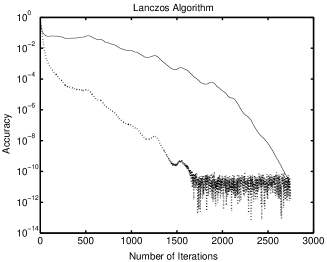
Figure 1: Normalized recursive residual (solid line) and relative differences of (4.14) (dotted line) produced by Algorithm 2.

To illustrate this situation we give an example from a $12^{3}\times 24$ lattice with $\mu=0.2$, bare quark mass $m_{q}=-0.869$ and a $SU(3)$ gauge field background at bare gauge coupling $\beta=5.9$. We compute the bilinear form (4.1) for:

$$f(s)=\log\tanh\sqrt{s},~{}~{}~{}~{}~{}s\in\mathbb{R}_{+}$$ (4.15)

and $A=H_{W}(m_{q},U)^{2}$, $b\in\text{I\kern-1.80832ptR}^{N}$ and $b-$elements are chosen randomly from the set $\{+1,-1\}$.

In Fig. 1 are shown the normalized recursive residuals $\left\|b-Ax_{i}\right\|_{2}/\left\|b\right\|_{2}$, $i=1,\ldots,n$ and relative differences of (4.14) between two successive Lanczos steps. The figure illustrates clearly the different regimes of convergence for the linear system and the bilinear form. The relative differences of the bilinear form converge faster than the computed recursive residual. This example indicates that a stopping criterion based on the solution of the linear system may indeed be strong and demanding. Therefore, the recommended stopping criteria would be to monitor the relative differences of the bilinear form but less frequently than proposed by Bai et al, (1996). More investigations are needed to settle this issue. Note also the roundoff effects (see Fig. 1) in the convergence of the bilinear form which are a manifestation of the finite precision of the machine arithmetic.

5 The link between overlap and domain wall fermions

Wilson regularization of quarks violates chiral symmetry even for massless quarks. This is a serious problem if we would like to compute mass spectrum with light sea quarks. The improvement of the discretization helps to reduce chiral symmetry breaking terms for a Wilson fermion. However, one must go close to the continuum limit in order to benefit from the improvement programme. This is not affordable with the present computing power.

The idea of Kaplan (1992) opened the door for chiral symmetry realization at finite lattice spacing. Narayanan and Neuberger (1993) proposed overlap fermions and Furman and Shamir (1995) domain wall fermions as a theory of chiral fermions on the lattice. The overlap operator is defined by Neuberger (1998):

$$D(m_{q},U)=\frac{1+m_{q}}{2}\text{1\kern-2.41109ptl}+\frac{1-m_{q}}{2}\gamma_{5}\text{sign}[H_{W}(M,U)]$$ (5.1)

with $M\in(-2,0)$ which is called the domain wall height, which substitutes the original bare quark mass of Wilson fermions. From now on we suppress the dependence on $M,m_{q}$ and $U$ of lattice operators for the ease of notations.

Domain wall fermions are lattice fermions in 5-dimensional Euclidean space time similar to the 4-dimensional formulation of Wilson fermions but with special boundary conditions along the fifth dimension. The 5-dimensional domain wall operator can be given by the $L_{5}\times L_{5}$ blocked matrix:

$$\mathcal{M}=\begin{pmatrix}a_{5}D_{W}-\text{1\kern-2.41109ptl}&P_{+}&&-m_{q}P_{-}\\ P_{-}&a_{5}D_{W}-\text{1\kern-2.41109ptl}&\ddots&\\ &\ddots&\ddots&P_{+}\\ -m_{q}P_{+}&&P_{-}&a_{5}D_{W}-\text{1\kern-2.41109ptl}\\ \end{pmatrix},~{}~{}~{}P_{\pm}=\frac{\text{1\kern-2.41109ptl}_{4}+\gamma_{5}}{2}$$

where the blocks are matrices defined on the 4-dimensional lattices and $P_{\pm}$ are $4\times 4$ chiral projection operators. Their presence in the blocks with dimensions $N\times N$ should be understood as the direct product with the colour and lattice coordinate spaces. $a_{5}$ is the lattice spacing along the fifth dimension.

These two apparently different formulations of chiral fermions are in fact closely related to each other Boriçi (1999). To see this we must calculate for the domain wall fermions the low energy effective fermion matrix in four dimensions. This can be done by calculating the transfer matrix $T$ along the fifth dimension. Multiplying $\mathcal{M}$ from the right by the permutation matrix:

$$\begin{pmatrix}P_{+}&P_{-}&&\\ &P_{+}&\ddots&\\ &&\ddots&P_{-}\\ P_{-}&&&P_{+}\\ \end{pmatrix}$$

we obtain:

$$\gamma_{5}\begin{pmatrix}(a_{5}H_{W}P_{+}-\text{1\kern-2.41109ptl})(P_{+}-m_{q}P_{-})&a_{5}H_{W}P_{-}+\text{1\kern-2.41109ptl}&&\\ &a_{5}H_{W}P_{+}-\text{1\kern-2.41109ptl}&\ddots&\\ &&\ddots&a_{5}H_{W}P_{-}+\text{1\kern-2.41109ptl}\\ (a_{5}H_{W}P_{-}+\text{1\kern-2.41109ptl})(P_{-}-m_{q}P_{+})&&&a_{5}H_{W}P_{+}-\text{1\kern-2.41109ptl}\\ \end{pmatrix}$$

Further, multiplying this result from the left by the inverse of the diagonal matrix:

$$\begin{pmatrix}a_{5}H_{W}P_{+}-\text{1\kern-2.41109ptl}&&&\\ &a_{5}H_{W}P_{+}-\text{1\kern-2.41109ptl}&&\\ &&\ddots&\\ &&&a_{5}H_{W}P_{+}-\text{1\kern-2.41109ptl}\\ \end{pmatrix}$$

we get:

$$\mathcal{T}(m):=\begin{pmatrix}P_{+}-m_{q}P_{-}&-T&&\\ &\text{1\kern-2.41109ptl}&\ddots&\\ &&\ddots&-T\\ -T(P_{-}-m_{q}P_{+})&&&\text{1\kern-2.41109ptl}\\ \end{pmatrix}$$ (5.2)

with the transfer matrix $T$ defined by:

$$T=\frac{\text{1\kern-2.41109ptl}}{\text{1\kern-2.41109ptl}-a_{5}H_{W}P_{+}}(\text{1\kern-2.41109ptl}+a_{5}H_{W}P_{-})$$

By requiring the transfer matrix being in the form:

$$T=\frac{\text{1\kern-2.41109ptl}+a_{5}\mathcal{H_{W}}}{\text{1\kern-2.41109ptl}-a_{5}\mathcal{H_{W}}}$$

it is easy to see that Boriçi (1999):

$$\mathcal{H_{W}}=H_{W}\frac{1}{2-a_{5}D_{W}}$$ (5.3)

Finally to derive the four dimensional Dirac operator one has to compute the determinant of the effective fermion theory in four dimensions:

$$\det D^{(L_{5})}=\frac{\det\mathcal{T}(m_{q})}{\det\mathcal{T}(1)}$$

where the subtraction in the denominator corresponds to a 5-dimensional theory with anti-periodic boundary conditions along the fifth dimension. It is easy to show that the determinant of the $L_{5}\times L_{5}$ block matrix $\mathcal{T}(m_{q})$ is given by:

$$\det\mathcal{T}(m_{q})=\det[(P_{+}-m_{q}P_{-})-T^{L_{5}}(P_{-}-m_{q}P_{+})]$$

or

$$\det\mathcal{T}(m_{q})=\det[\frac{1+m_{q}}{2}\gamma_{5}(\text{1\kern-2.41109ptl}+T^{L_{5}})+\frac{1-m_{q}}{2}(\text{1\kern-2.41109ptl}-T^{L_{5}})]$$

which gives:

$$D^{(L_{5})}=\frac{1+m_{q}}{2}\text{1\kern-2.41109ptl}+\frac{1-m_{q}}{2}\gamma_{5}\frac{\text{1\kern-2.41109ptl}-T^{L_{5}}}{\text{1\kern-2.41109ptl}+T^{L_{5}}}$$ (5.4)

In the large $L_{5}$ limit one gets the Neuberger operator (5.1) but now the operator $H_{W}$ substituted with the operator $\mathcal{H}_{W}$ (5.3). Taking the continuum limit in the fifth dimension one gets ${\mathcal{H}_{W}}\rightarrow H_{W}$. This way overlap fermions are a limiting theory of the domain wall fermions. To achieve the chiral properties as in the case of overlap fermions one must take the large $L_{5}$ limit in the domain wall formulation.

One can ask the opposite question: is it possible to formulate the overlap in the form of the domain wall fermions? The answer is yes and this is done using truncated overlap fermions Boriçi 2000c . The corresponding domain wall matrix is given by:

$${\mathcal{M}}_{TOV}=\begin{pmatrix}a_{5}D_{W}-\text{1\kern-2.41109ptl}&(a_{5}D_{W}+\text{1\kern-2.41109ptl})P_{+}&&-m_{q}(a_{5}D_{W}+\text{1\kern-2.41109ptl})P_{-}\\ (a_{5}D_{W}+\text{1\kern-2.41109ptl})P_{-}&a_{5}D_{W}-\text{1\kern-2.41109ptl}&\ddots&\\ &\ddots&\ddots&(a_{5}D_{W}+\text{1\kern-2.41109ptl})P_{+}\\ -m_{q}(a_{5}D_{W}+\text{1\kern-2.41109ptl})P_{+}&&(a_{5}D_{W}+\text{1\kern-2.41109ptl})P_{-}&a_{5}D_{W}-\text{1\kern-2.41109ptl}\\ \end{pmatrix}$$

The transfer matrix of truncated overlap fermions is calculated using the same steps as above. One gets:

$$T_{TOV}=\frac{\text{1\kern-2.41109ptl}+a_{5}H_{W}}{\text{1\kern-2.41109ptl}-a_{5}H_{W}}$$

The 4-dimensional Dirac operator has the same form as the corresponding operator of the domain wall fermion (5.4) where $T$ is substituted with $T_{TOV}$ (or $\mathcal{H}_{W}$ with $H_{W}$). Therefore the overlap Dirac operator (5.1) is recovered in the large $L_{5}$ limit.

6 A two-level algorithm for overlap inversion

In this section we review the two-level algorithm of Boriçi 2000d . The basic stucture of the algorithm is that of a preconditioned Jacobi:

$$x^{i+1}=x^{i}+S_{n}^{-1}(b-Dx^{i}),~{}~{}~{}i=0,1,\ldots$$ (6.1)

where $S_{n}$ is the preconditioner of the overlap operator $D$ given by:

$$S_{n}=\frac{1+m_{q}}{2}\text{1\kern-2.41109ptl}+\frac{1-m_{q}}{2}\gamma_{5}H_{W}\sum_{k=1}^{n}\frac{a_{k}}{H_{W}^{2}+b_{k}\text{1\kern-2.41109ptl}}$$ (6.2)

where $a_{k},b_{k}\in\mathbb{R},k=1,\ldots,n$ are coefficients that can be optimized to give the best rational approximation of the $sign(H_{W})$ with the least number of terms in the right hand side. For example one can use the optimal rational approximation coefficients of Zolotarev Zolotarev (1877); Petrushev and Popov (1987). For the rational approximation of $sign(H_{W})$ one has:

$$D=\lim_{n\rightarrow\infty}S_{n}$$ (6.3)

In order to compute efficiently the inverse of the preconditioner we go back to the 5-dimensional formulation of the overlap operator (see the previous section as well) which can be written as a matrix in terms of 4-dimensional block matrices:

$${\cal H}=\begin{pmatrix}\frac{1+m_{q}}{2}\text{1\kern-2.41109ptl}&\frac{1-m_{q}}{2}\gamma_{5}H_{W}&\cdots&\frac{1-m_{q}}{2}\gamma_{5}H_{W}\\ -a_{1}\text{1\kern-2.41109ptl}&H_{W}^{2}+b_{1}\text{1\kern-2.41109ptl}&&\\ \vdots&&\ddots&\\ -a_{n}\text{1\kern-2.41109ptl}&&&H_{W}^{2}+b_{n}\text{1\kern-2.41109ptl}\\ \end{pmatrix}$$ (6.4)

This matrix can be also partitioned in the $2\times 2$ blocked form:

$${\cal H}=\begin{pmatrix}H_{11}&H_{12}\\ H_{21}&H_{22}\\ \end{pmatrix}$$ (6.5)

with Schur complement:

$$S_{11}=H_{11}-H_{12}H_{22}^{-1}H_{21}$$ (6.6)

It is easy to show that the following statements hold:

Proposition 6.1

i) The preconditioner $S_{n}$ is given by the Schur complement:

$$S_{n}=S_{11}$$ (6.7)

ii) Let ${\cal H}\chi=\eta$ with $\chi=(y,\chi_{1},\ldots,\chi_{n})^{T}$ and $\eta=(r,o,\ldots,o)^{T}$. Then $y$ is the solution of the linear system $S_{n}y=r$.

Using these results and keeping $n$ fixed the algorithm of Boriçi 2000d (known also as the multigrid algorithm) has the form of a two level algorithm:

Algorithm 3    A two-level algorithm for overlap inversion

  Set $x^{1}\in\mathbb{C}^{N},~{}r^{1}=b,~{}\text{tol}\in\mathbb{R}_{+},~{}\text{tol}_{1}\in\mathbb{R}_{+}$

  for $~{}i=1,\ldots$ do

     Solve approximately  ${\cal H}\chi^{i+1}=\eta^{i}$ such that $||\eta^{i}-{\cal H}\chi^{i+1}||_{2}/||r^{i}||_{2}<\text{tol}_{1}$

     $x^{i+1}=x^{i}+y^{i+1}$

     $r^{i+1}=b-Dx^{i+1}$

     Stop if $||r^{i+1}||_{2}/||b||_{2}<$ tol

  end for

This algorithm is in the form of nested iterations. One can see that the outer loop is Jacobi iteration which contains inside two inner iterations: the approximate solution of the 5-dimensional system and the multiplication with the overlap operator $D$ which involves the computation of the $sign$ function. For the 5-dimensional system one can use any iterative solver which suites the properties of $\cal H$. We have used many forms for $\cal H$ ranging from rational approximation to domain wall formulations. For the overlap multiplication we have used the algorithm of Boriçi, 2000b . Our test on a small lattice show that the two level algorithm outperforms with an order of magnitude the brute force conjugate gradients nested iterations Boriçi 2000d .

Since the inner iteration solves the problem in a 5-dimensional lattice with finite $L_{5}$ and the outer iteration solves for the 4-dimensional projected 5-dimensional system with $L_{5}\rightarrow\infty$, the algorithm in its nature is a multigrid algorithm along the fifth dimension. The fact that the multigrid works here is simply the free propagating fermions in this direction. If this direction is gauged, the usual problems of the multigrid on a 4-dimensional lattice reappear and the idea does not work. In fact, this algorithm with $n$ fixed is a two grid algorithm. However, since it does not involve the classical prolongations and contractions it can be better described as a two-level algorithm.

References

- Wilson (1974) K.G. Wilson, Confinement of quarks, Phys. Rev. D 10 (1974) pp. 2445-2459
- Wasilkowski and Woźniakowski (1996) G. W. Wasilkowski and H. Woźniakowski, On tractability of path integration, J. Math. Phys. 37 (1994) pp. 2071-2086
- Peardon (2003) Monte Carlo Algorithms for QCD, this volume.
- Weingarten and Petcher (1981) D.H. Weingarten and D.N. Petcher, Monte Carlo integration for lattice gauge theories with fermions, Phys. Lett. B99 (1981) 333
- Boriçi and de Forcrand (1994) A. Boriçi and Ph. de Forcrand, Fast Methods for Calculation of Quark Propagator, Physics Computing 1994, p.711.
- Frommer et al (1994) Accelerating Wilson Fermion Matrix Inversions by Means of the Stabilized Biconjugate Gradient Algorithm, A. Frommer, V. Hannemann, Th. Lippert, B. Noeckel, K. Schilling, Int.J.Mod.Phys. C5 (1994) 1073-1088
- Bai et al, (1996) Z. Bai, M. Fahey, and G. H. Golub, Some large-scale matrix computation problems, J. Comp. Appl. Math., 74:71-89, 1996
- Thron et al (1998) C. Thron, S.J. Dong, K.F. Liu, H.P. Ying, Padé-Z2 estimator of determinants Phys. Rev. D57 (1998) pp. 1642-1653
- Cahill et al, (1999) E. Cahill, A. Irving, C. Johnson, J. Sexton, Numerical stability of Lanczos methods, Nucl. Phys. Proc. Suppl. 83 (2000) 825-827
- (10) , A. Boriçi, Computational Methods for UV-Suppressed Fermions, J. Comp. Phys.189 (2003) 454-462
- (11) A. Boriçi, Lattice QCD with Suppressed High Momentum Modes of the Dirac Operator, Phys. Rev. D67(2003) 114501
- Golub (2003) G. Golub, Variance Reduction by Control Variates in Monte Carlo Simulations of Large Scale Matrix Functions, this volume.
- (13) A. Boriçi, Global Monte Carlo for Light Quarks, to be published in the Nuc. Phys. B proceedings of the XXI International Symposium on Lattice Field Theory, Tsukuba, Ibaraki, Japan. See also physics archives hep-lat/0309044.
- (14) A. Boriçi, Determinant and Order Statistics, this volume.
- (15) A. Boriçi, On the Neuberger overlap operator, Phys. Lett. B453 (1999) 46-53
- (16) A. Boriçi, Fast methods for computing the Neuberger Operator, in A. Frommer et al (edts.), Numerical Challenges in Lattice Quantum Chromodynamics, Springer Verlag, Heidelberg, 2000.
- (17) A. Boriçi, A Lanczos approach to the Inverse Square Root of a Large and Sparse Matrix, J. Comput. Phys. 162 (2000) 123-131
- Lanczos, (1952) C. Lanczos, Solution of systems of linear equations by minimized iterations, J. Res. Nat. Bur. Stand., 49 (1952), pp. 33-53
- Graves-Morris, (1979) P. R. Graves-Morris, Padé Approximation and its Applications, Lecture Notes in Mathematics, vol. 765, L. Wuytack, ed.. Springer Verlag, 1979
- Freund, (1993) R. W. Freund, Solution of Shifted Linear Systems by Quasi-Minimal Residual Iterations, in L. Reichel and A. Ruttan and R. S. Varga (edts), Numerical Linear Algebra, W. de Gruyter, 1993
- Golub & Strakos (1994) G. H. Golub and Z. Strakos, Estimates in quadratic formulas, Numerical Algorithms, 8 (1994) pp. 241-268.
- Golub & Van Loan, (1989) G. H. Golub and C. F. Van Loan, Matrix Computations, The Johns Hopkins University Press, Baltimore, 1989
- Bai et al edts, (2000) Z. Bai et al editors, Templates for the Solution of Algebraic Eigenvalue Problems: A Practical Guide (Software, Environments, Tools), SIAM, 2000.
- Kaplan (1992) D.B. Kaplan, A Method for Simulating Chiral Fermions on the Lattice Phys. Lett. B 228 (1992) 342.
- Narayanan and Neuberger (1993) R. Narayanan, H. Neuberger, Infinitely many regulator fields for chiral fermions, Phys. Lett. B 302 (1993) 62, A construction of lattice chiral gauge theories, Nucl. Phys. B 443 (1995) 305.
- Furman and Shamir (1995) V. Furman, Y. Shamir, Axial symmetries in lattice QCD with Kaplan fermions, Nucl. Phys. B439 (1995) 54-78
- Neuberger (1998) H. Neuberger, Exactly massless quarks on the lattice, Phys. Lett. B 417 (1998) 141
- Boriçi (1999) A. Boriçi, Truncated Overlap Fermions: the link between Overlap and Domain Wall Fermions, in V. Mitrjushkin and G. Schierholz (edts.), Lattice Fermions and Structure of the Vacuum, Kluwer Academic Publishers, 2000.
- (29) A. Boriçi, Truncated Overlap Fermions, Nucl. Phys. Proc. Suppl. 83 (2000) 771-773
- (30) A. Boriçi, Chiral Fermions and the Multigrid Algorithm, Phys. Rev. D62 (2000) 017505
- Zolotarev (1877) E. I. Zolotarev, Application of the elliptic functions to the problems on the functions of least and most deviation from zero, Zapiskah Rossijskoi Akad. Nauk. (1877). In Russian.
- Petrushev and Popov (1987) P.P. Petrushev and V.A. Popov, Rational approximation of real functions, Cambridge University Press, Cambridge 1987.