Perturbation theory vs. simulation for tadpole improvement factors in pure gauge theories

Abstract

We calculate the mean link in Landau gauge for Wilson and improved $SU(3)$ anisotropic gauge actions, using two loop perturbation theory and Monte Carlo simulation employing an accelerated Langevin algorithm. Twisted boundary conditions are employed, with a twist in all four lattice directions considerably improving the (Fourier accelerated) convergence to an improved lattice Landau gauge. Two loop perturbation theory is seen to predict the mean link extremely well even into the region of commonly simulated gauge couplings and so can be used remove the need for numerical tuning of self-consistent tadpole improvement factors. A three loop perturbative coefficient is inferred from the simulations and is found to be small. We show that finite size effects are small and argue likewise for (lattice) Gribov copies and double Dirac sheets.

I Introduction

Tadpole improvement is now widespread in lattice field theory Lepage:1993xa . Without it, lattice perturbation theory begins to fail on distance scales of order 1/20 fm. Perturbation theory in other regularisations, however, seems to be phenomenologically successful down to energy scales of the order of 1 GeV (corresponding to lattice spacings of 0.6 fm) Lepage:1996jw .

The reason is that the bare lattice coupling is too small Lepage:1993xa ; Lepage:1996jw . To describe quantities dominated by momenta of order the cut-off scale ($\pi/a$), it is appropriate to expand in the running coupling, $\alpha_{s}$, evaluated at that scale. The bare coupling, however, deviates markedly from this and its anomalously small value at finite lattice spacing can be associated with tadpole corrections Lepage:1996jw . These tadpole corrections are generally process independent and can be (largely) removed from all quantities by modifying the action. This corresponds to a resumming of the perturbative series to yield an expansion in powers of a new, “boosted” coupling that is much closer to $\alpha_{s}(\pi/a)$.

Perturbatively this amounts to adding a series of radiative counterterms to the action. Such a series is obtained by dividing each gauge link in the action by an appropriate expansion, $u^{(\mathrm{PT})}$. It is sufficient that this series is known only up to the loop order of the other quantities we wish to calculate using the action.

The factor $u^{(\mathrm{PT})}$ is not unique, but it should clearly be dominated by ultraviolet fluctuations on the scale of the cut-off. The two most common definitions are the fourth root of the mean plaquette (a gauge invariant definition) and the expectation value of the link in Landau gauge. Both are successful, although lattice results suggest some arguments for preferring the latter Lepage:1998id . In this paper we discuss Landau gauge mean link tadpole improvement.

For Monte Carlo simulations, each gauge link in the action is divided by a numerical factor, $u^{(\mathrm{MC})}$. Its value is fixed by a self–consistency criterion; the value measured in the simulation should agree with the parameter in the action. Obtaining such numerical agreement requires computationally expensive tuning of the action. In many cases this cost is prohibitive, such as the zero temperature tuning of highly anisotropic actions for use in finite temperature simulations. As non–perturbative phenomena should not affect the cut-off scale, a sufficiently high order perturbative series should predict $u^{(\mathrm{MC})}$ such that the subsequent numerical tuning is unnecessary.

In this paper we present the tadpole improvement factors calculated to two loop order using lattice perturbation theory. This covers the loop order of most perturbative calculations using lattice actions. In addition, we perform Monte Carlo simulations over a range of gauge couplings extending from the high-$\beta$ regime down to the lattice spacings used in typical simulations. We demonstrate that the two loop formula predicts the numerically self–consistent $u^{(\mathrm{MC})}$ to within a few digits of the fourth decimal place and the additional tuning required is minimal (especially when the action can be rescaled as in Drummond:2002yg ; Drummond:2003qu ). For this reason we refer to both $u^{(\mathrm{PT})}$ and $u^{(\mathrm{MC})}$ as $u$ from hereonin. The small deviations at physical couplings are shown to be consistent with a third order correction to $u$ and we infer the coefficient of this. In most cases no tuning at all is required if the third order is included.

These calculations are carried out for two $SU(3)$ lattice gauge actions; the Wilson action and a first order Symanzik improved action. Isotropic and anisotropic lattices are studied and interpolations of the coefficients with the anisotropy are given.

The structure of this paper is as follows. We first discuss the perturbative calculation in Section II. In Section III we describe high-$\beta$ Monte Carlo simulations, and use the results to obtain higher order coefficients in the perturbative expansion, before concluding in Section IV. A brief description of twisted boundary conditions is given in Appendix A.

The results presented here extend and, in some cases, correct the preliminary results presented in Drummond:2002kp . Extension of this work to actions including fermions is being carried out and will be reported in a future publication.

II Perturbation theory

We write the Landau gauge mean links

$$u_{\mu}=\left\langle\mathop{\mathrm{tr}}U_{\mu}\right\rangle$$ (1)

(where $N$ is the number of colours and $\mathop{\mathrm{tr}}\equiv\frac{1}{N}\mathop{\mathrm{Tr}}$) as

$$u_{\mu}=1+a^{(1)}_{\mu}g^{2}+a^{(2)}_{\mu}g^{4}+{\cal O}(g^{6})\;.$$ (2)

Using an anti-Hermitian gauge potential, $U_{\mu}=\exp gA_{\mu}$, the mean Landau link in perturbation theory is

$$\left\langle\mathop{\mathrm{tr}}U_{\mu}\right\rangle=1+g^{2}\left\langle\mathop{\mathrm{tr}}\frac{A_{\mu}^{2}}{2}\right\rangle+g^{4}\left\langle\mathop{\mathrm{tr}}\frac{A_{\mu}^{4}}{24}\right\rangle+{\cal O}(g^{6})\;.$$ (3)

We use twisted boundary conditions to regulate the gluon zero mode in a gauge invariant manner. A brief resumé of relevant results and definitions is given in Appendix A and the reader is referred to luwe ; Drummond:2002yg for a fuller discussion.

Figure 1: Feynman diagrams for the mean link.

Figure 2: Feynman diagrams for the gluon self energy, $\Sigma_{\mu\nu}$. Feynman rules are discussed in Drummond:2002yg .

II.1 one loop

The one loop contribution comes from

$$\left\langle\mathop{\mathrm{tr}}A_{\mu}^{2}\right\rangle = \frac{1}{N}\frac{1}{V_{TW}^{2}}\sum_{\bm{k},\bm{p}}e^{i\left(\bm{k}+\bm{p}\right)\cdot\bm{x}}$$ (4)

$$\times\mathop{\mathrm{Tr}}\left[\Gamma(\bm{k})\Gamma(\bm{p})\right]\tilde{A}_{\mu}(\bm{k})\tilde{A}_{\mu}(\bm{p})\;.$$

The one loop coefficient is thus the sum over the tree level propagator in Landau gauge (see Eqn. (18) of Drummond:2002yg ),

$$a^{(1)}_{\mu}=\frac{1}{2V_{TW}}\sum_{\bm{k}}z^{\frac{1}{2}(\bm{k},\bm{k})}G_{\mu\mu}(\bm{k})\;,$$ (5)

shown in Fig. 1. We note here that the phase in the integrand is precisely that of the inverse propagator in the twisted formalism (see Eqn. (63) of Drummond:2002yg ), so $a^{(1)}_{\mu}$ is real.

Table 1: One loop coefficients for various anisotropies, $\chi$, extrapolated to infinite lattice size, $L$.

action	anisotropy	$a^{(1)}_{s}$	$a^{(1)}_{t}$
Wilson	1.0	-0.077467	-0.077467
	1.25	-0.087488	-0.051452
	1.5	-0.095096	-0.036299
	2.0	-0.105351	-0.020351
	2.5	-0.111543	-0.012886
	3.0	-0.115452	-0.008851
	4.0	-0.119871	-0.004899
	6.0	-0.123393	-0.002142
	8.0	-0.124713	-0.001197
Symanzik	1.0	-0.063049	-0.064664
improved	1.25	-0.071472	-0.042877
	1.5	-0.077940	-0.030150
	2.0	-0.086772	-0.016934
	2.42	-0.091467	-0.011462
	2.5	-0.092171	-0.010720
	2.78	-0.094281	-0.008616
	3.0	-0.095620	-0.007365
	3.5	-0.097922	-0.005363
	4.0	-0.099521	-0.004077
	5.0	-0.10152	-0.002584
	6.0	-0.10266	-0.001784
	8.0	-0.10384	-0.000997

II.2 two loops

The two loop contribution arises from two sources. The first is from the above integral, Eqn. (5), where the tree level propagator is replaced by the one loop self energy bubble shown in Fig. 2, giving a term

$$a_{\mu}^{(2)} = \frac{1}{2V_{TW}}\sum_{\bm{k}}z^{\frac{1}{2}(\bm{k},\bm{k})}G_{\mu\alpha}(\bm{k})\Sigma_{\alpha\beta}(\bm{k})G_{\beta\mu}(\bm{k})$$ (6)

$$+\mathrm{~{}Eqn.~{}(\ref{eqn_fig8_terms}).}$$

As $\Sigma_{\alpha\beta}$ has the phase of the inverse propagator, this expression is also explicitly real.

Table 2: Two loop coefficients for various anisotropies, $\chi$, extrapolated to infinite lattice size, $L$.

action	anisotropy	$a^{(2)}_{s}$	$a^{(2)}_{t}$	$b^{(2)}_{s}$	$b^{(2)}_{t}$
Wilson	1.0	-0.021093 (63)	-0.021093 (63)	0.002912 (63)	0.002912 (63)
	1.25	-0.023891 (74)	-0.013222 (91)	0.003573 (74)	0.002930 (91)
	1.5	-0.025721 (95)	-0.008913 (63)	0.004861 (95)	0.002760 (63)
	2.0	-0.027669 (91)	-0.004730 (37)	0.007771 (91)	0.002116 (37)
	2.5	-0.02827 (11)	-0.002900 (23)	0.01049 (11)	0.001578 (23)
	3.0	-0.02839 (12)	-0.001916 (16)	0.01262 (12)	0.001228 (16)
	4.0	-0.02811 (13)	-0.001008 (14)	0.01558 (13)	0.000778 (14)
	6.0	-0.02718 (27)	-0.0004080 (42)	0.01876 (27)	0.0000377 (42)
Symanzik	1.0	-0.01327 (23)	-0.01435 (24)	0.00273 (23)	0.00206 (24)
improved	2.0	-0.01831 (34)	-0.003444 (63)	0.00574 (34)	0.001251 (63)
	3.0	-0.01931 (50)	-0.001456 (30)	0.00882 (50)	0.000711 (30)
	4.0	-0.02011 (53)	-0.0010482 (181)	0.01001 (53)	0.0001857 (181)

The second term arises from the tree level portion of the $A_{\mu}^{4}$ term:

$$\left\langle\mathop{\mathrm{tr}}A_{\mu}^{4}\right\rangle = \frac{1}{N}\frac{1}{V_{TW}^{4}}\sum_{\bm{k}_{1}...\bm{k}_{4}}\exp\left[i(\bm{k}_{1}+...+\bm{k}_{4})\cdot\bm{x}\right]$$ (7)

$$\times\mathop{\mathrm{Tr}}\left[\Gamma(\bm{k}_{1})...\Gamma(\bm{k}_{4})\right]\tilde{A}_{\mu}(\bm{k}_{1})...\tilde{A}_{\mu}(\bm{k}_{4}).$$

Using Eqn. (58), this reduces to

$$a_{\mu}^{(2)} = \mathrm{~{}Eqn.~{}(\ref{eqn_vegas_terms})}$$ (8)

$$+~{}\frac{1}{24V_{TW}^{2}}\sum_{\bm{k},\bm{p}}\left(2+z^{\langle\bm{k},\bm{p}\rangle}\right)z^{\frac{1}{2}(\bm{k},\bm{k})}G_{\mu\mu}(\bm{k})$$

$$~{}~{}~{}\times z^{\frac{1}{2}(\bm{p},\bm{p})}G_{\mu\mu}(\bm{p})\;.$$

Since the integrand is symmetric in $\bm{k}$ and $\bm{p}$, only the real, cosine part of $z^{\langle\bm{k},\bm{p}\rangle}$ survives and the integral is real.

As $\langle\bm{k},\bm{p}\rangle$ depends only on the twist components of $\bm{k},\bm{p}$, we note that if

$$\sum_{\bar{\bm{k}}}z^{\frac{1}{2}(\bm{k},\bm{k})}G_{\mu\mu}(\bm{k})$$ (9)

is stored for each possible value of the associated twist vector (see Appendix for the definition of $\bar{\bm{k}}$), the second expression in Eqn. (8) can be reduced to the product of two one–loop calculations.

Table 3: Contributions to the two loop coefficients, $a^{(2)}_{s,t}$. The notation used in labelling the contributions is explained in the text.

action	coefficient	anisotropy	VEGAS	Figure of 8	$a^{(1)}_{s}\Delta S_{ct}$	$\Delta S_{ct}$
Wilson	$a^{(2)}_{s}$	1.0	-0.022969 (63)	0.001875
		1.25	-0.026283 (74)	0.002392
		1.5	-0.028547 (95)	0.002826
		2.0	-0.031138 (91)	0.003468
		2.5	-0.03216 (11)	0.003888
		3.0	-0.03255 (12)	0.004166
		4.0	-0.03260 (13)	0.04488
		6.0	-0.03194 (27)	0.004759
	$a^{(2)}_{t}$	1.0	-0.022969 (63)	0.001875
		1.25	-0.014049 (91)	0.000827
		1.5	-0.009323 (63)	0.000410
		2.0	-0.004859 (37)	0.000130
		2.5	-0.002952 (23)	0.000052
		3.0	-0.001941 (16)	0.000025
		4.0	-0.001015 (14)	0.000008
		6.0	-0.0004095 (42)	0.000002
Symanzik	$a^{(2)}_{s}$	1.0	-0.01232 (23)	0.0012422	-0.0021920	0.034766
improved		2.0	-0.01693 (34)	0.0023529	-0.0037334	0.043026
		3.0	-0.01780 (50)	0.0028573	-0.0043696	0.045697
		4.0	-0.01855 (53)	0.0030951	-0.0046588	0.046811
	$a^{(2)}_{t}$	1.0	-0.01468 (24)	0.00130671	-0.00097386	0.015446
		2.0	-0.003193 (63)	0.00008961	-0.00034017	0.0039203
		3.0	-0.00131 (30)	0.00001695	-0.00016325	0.0017073
		4.0	-0.0009590 (181)	0.00000520	-0.00009436	0.0009481

II.3 Numerical integration

We consider the lattice Wilson action (W) and the Symanzik improved action (SI) defined in alea , both with tadpole improvement in the spatial ($s$) and temporal ($t$) directions.

$$S_{W} (\beta_{0},\chi_{0},u_{s},u_{t})=-\frac{\beta_{0}}{\chi_{0}}\sum_{x,s>s^{\prime}}\frac{P_{s,s^{\prime}}}{u_{s}^{4}}-\beta_{0}\chi_{0}\sum_{x,s}\frac{P_{s,t}}{u_{s}^{2}u_{t}^{2}}$$

$$S_{SI} (\beta_{0},\chi_{0},u_{s},u_{t})=$$ (10)

$$-\frac{\beta_{0}}{\chi_{0}}\sum_{x,s>s^{\prime}}{\left(\frac{5}{3}\frac{P_{s,s^{\prime}}}{u_{s}^{4}}-\frac{1}{12}\frac{R_{ss,s^{\prime}}}{u_{s}^{6}}-\frac{1}{12}\frac{R_{s^{\prime}s^{\prime},s}}{u_{s}^{6}}\right)}$$

$$-\beta_{0}\chi_{0}\sum_{x,s}{\left(\frac{4}{3}\frac{P_{s,t}}{u_{s}^{2}u_{t}^{2}}-\frac{1}{12}\frac{R_{ss,t}}{u_{s}^{4}u_{t}^{2}}\right)}\;,$$

where $s,s^{\prime}$ run over spatial links; $P_{s,s^{\prime}}$ and $P_{s,t}$ are $1\times 1$ plaquettes; $R_{ss,s^{\prime}}$ and $R_{ss,t}$ are $2\times 1$ loops; and $\chi_{0}$ is the bare anisotropy.

It is clearly inconvenient to work perturbatively with actions whose parameters are implicit functions of the expansion parameter $g_{0}^{2}$. To circumvent this problem we define

$$\beta=\beta_{0}/(u_{s}^{3}u_{t})\;,~{}~{}g^{2}=g_{0}^{2}u_{s}^{3}u_{t}\;,~{}~{}\chi=\chi_{0}u_{s}/u_{t}\;,$$ (11)

and find

$$S_{W} (\beta_{0},\chi_{0},u_{s},u_{t})=S_{W}(\beta,\chi,u_{s}=u_{t}=1)\;,$$

$$S_{SI} (\beta_{0},\chi_{0},u_{s},u_{t})~{}=~{}S_{SI}(\beta,\chi,u_{s}=u_{t}=1)~{}+$$

$$g^{2}\Delta S_{SI}+{\cal O}(g^{4})\;,$$

$$\Delta S_{SI} =d_{s}\Delta S_{ct}$$ (12)

$$=d_{s}\beta\sum_{\stackrel{{\scriptstyle x}}{{s>s^{\prime}}}}\frac{1}{6}\left(\frac{\left[R_{ss,s^{\prime}}+R_{s^{\prime}s^{\prime},s}\right]}{\chi}+\chi R_{ss,t}\right),$$

where $d_{s}$ is the one loop coefficient in the (self-consistent) perturbative expansion of the tadpole improvement factor. For mean Landau link improvement $d_{s}=a^{(1)}_{s}$.

Perturbative expansions will initially be calculated as power series in $g^{2}$ and the expansion then re-expressed as a series in $g_{0}^{2}$.

The Feynman rules are obtained by perturbatively expanding the lattice actions using an automated computer code written in Python luwe ; Drummond:2002kp . The additional vertices associated with the ghost fields and the measure for Landau gauge are given in luwe ; Drummond:2002yg . The Feynman diagrams for the one and two loop calculations are shown in Figs. 1 and 2.

The one loop integration is carried out by direct summation of all twisted momentum modes for hypercubic lattices with $4\leq L_{\mu}\leq 32$. To speed up the approach to infinite volume, the momenta are “squashed” in the directions with periodic boundary conditions using the change of variables $\bm{k}\rightarrow\bm{k}^{\prime}$ suggested by Lüscher and Weisz luwe

$$k^{\prime}_{\mu}=k_{\mu}-\alpha_{\mu}\;\hbox{sin}(k_{\mu})\;,$$ (13)

giving an integrand with much broader peaks which is easier to evaluate numerically. It is easy to see that a reasonable choice of parameter is $\alpha_{\mu}\sim 1-(\chi L_{\mu})^{-1}$ and significantly reduced the dependence on $L$. The calculations were all possible on a workstation.

All results were extrapolated to infinite volume using a fit function of the form $c_{0}+c_{1}/L^{2}$, which worked extremely well for $L\geq 16$. As a further check, the coefficients in the expansion of the spatial mean link should extrapolate to the same value in twisted and periodic directions. We found this to be the case, with the discrepancy much smaller than the number of significant figures quoted in the results in this paper.

We calculate the two loop coefficient in three parts. The “figure of 8” diagram from Eqn. (8) is calculated by mode summation using the reduction described above.

The remaining two loop calculations arising from Fig. 2$(a-d)$ (and from the trivial Fig. 2$e$) were carried out using Vegas, a Monte Carlo estimation program lepage78 ; numrec . With a version of Vegas parallelised using the MPI protocol, these computations were carried out on between 64 and 256 processors of a Hitachi SR2201 supercomputer. Each run took of the order of 24 hours. We label the results from this calculation “VEGAS”. We used the 2–twist boundary conditions described in the Appendix. The lattice was of infinite extent in the untwisted $\mu=3,4$ directions, and of size $L\in\{4,8,16,32\}$ in the twisted $\mu=1,2$ directions. Again, the Lüscher-Weisz squashing was applied to the untwisted momentum components.

Finally, for the Symanzik improved actions there is a counterterm insertion, Fig. 2$f$, arising from $\Delta S_{ct}$, which requires a one loop calculation carried out by mode summation. Multiplying this result by the appropriate $d_{s}$ gives the full contribution of the counterterm.

We show the one loop results in Table 1 and the two loop results for $d_{s}=a^{(1)}_{s}$ in Table 2. As it is possible that results for the mean link in Landau gauge from an action with a different tadpole improvement scheme might be desired (or an action with no improvement at all, when $d_{s}=0$), the contributions of the various parts of the two loop calculation are shown in Table 3 to allow the reader to construct the appropriate two loop contribution (the one loop numbers being unchanged) Drummond:2003qu .

Table 4: Fits to perturbative expansion coefficients as functions of $\chi$, as defined in the text.

action	quantity	const.	$1/\chi$	$1/\chi^{2}$	$\log\chi/\chi$
Wilson	$a_{s}^{(1)}=b_{s}^{(1)}$	-0.120648	0.103142	-0.0599588	-0.0614259
	$a_{t}^{(1)}=b_{t}^{(1)}$	0	-0.0168915	-0.0609128	0.00881346
	$a_{s}^{(2)}$	-0.0174148	0.0198738	-0.0235448	-0.0410654
	$a_{t}^{(2)}$	0	0.00384188	-0.024975	-0.00118467
	$b_{s}^{(2)}$	0.0296102	-0.041532	0.0148529	-0.0134185
	$b_{t}^{(2)}$	0	0.0180304	-0.0152916	-0.00847315
Symanzik	$a_{s}^{(1)}=b_{s}^{(1)}$	-0.10043	0.0915721	-0.0541941	-0.0536973
improved	$a_{t}^{(1)}=b_{t}^{(1)}$	0	-0.012287	-0.0526966	0.00656986
	$a_{s}^{(2)}$	-0.0300447	-0.0215242	0.038299	0.0372853
	$a_{t}^{(2)}$	0	0.00708635	-0.0214381	-0.00419861
	$b_{s}^{(2)}$	0.00122385	-0.0728384	0.0743446	0.0644862
	$b_{t}^{(2)}$	0	0.0129186	-0.0108602	-0.00676255

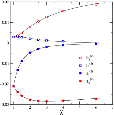
Figure 3: Two loop coefficients to the Landau mean link for the Wilson action.

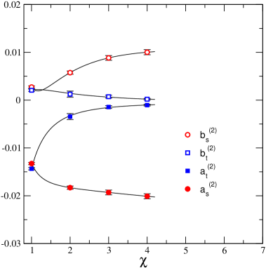
Figure 4: Two loop coefficients to the Landau mean link for the tadpole improved Symanzik action.

II.4 Resumming the series

Perturbatively speaking, tadpole improvement resums the perturbative expansion in the hope of reducing truncation errors in the series. This amounts to using $g_{0}^{2}$ as the expansion parameter, rather than $g^{2}$. Writing

$$u_{l}=\left\{\begin{array}[]{lll}1+a^{(1)}_{l}g^{2}&+a^{(2)}_{l}g^{4}&+{\cal O}(g^{6})\;,\\ 1+b^{(1)}_{l}g_{0}^{2}&+b^{(2)}_{l}g_{0}^{4}&+{\cal O}(g_{0}^{6})\;,\end{array}\right.$$ (14)

we find

$$b^{(1)}_{l} = a^{(1)}_{l}\;,$$

$$b^{(2)}_{l} = a^{(2)}_{l}+a^{(1)}_{l}(3a^{(1)}_{s}+a^{(1)}_{t})\;.$$ (15)

The coefficients $b^{(2)}_{s,t}$ for mean Landau link tadpole improvement are given in Table 2.

Finally, we carry out interpolating fits in the anisotropy, $\chi$, to all perturbative coefficients using the function

$$c_{0}+\frac{c_{1}}{\chi}+\frac{c_{2}}{\chi^{2}}+c_{3}\frac{\log\chi}{\chi}\;.$$ (16)

These fits work well. The fit parameters are given in Table 3 and are shown in Figs. 3 and 4. It should be noted when using these results that $\chi$ is the anisotropy after the majority of tadpole factors have been scaled out of the action, as is shown in Eqn. (12).

III Monte Carlo simulation

By comparing the truncated two loop perturbative series obtained above with results from high-$\beta$ Monte Carlo simulations, higher order coefficients in the perturbative expansion may be inferred Trottier:2001vj .

III.1 Implementing the Langevin update

Field configurations were generated using a 2nd order Runge-Kutta Langevin updating routine. The implementation of the Langevin evolution is such that any pure gauge action can be simulated by simply specifying the list of paths and the associated couplings. The group derivative for each loop is then computed automatically by an iterative procedure which moves around the loop link by link constructing the appropriate traceless anti-Hermitian contribution to the Langevin velocity. This is the most efficient implementation, minimising the number of group multiplications needed and can be applied whenever the quantity to be differentiated is specified as a (closed) Wilson path.

The method is as follows. We specify a given link by a start site, $x$, and a signed direction, $\mu$:

$$U_{\mu}({\mbox{\boldmath$x$}}) \mu>0\;,$$

$$U_{-\mu}^{\dagger}({\mbox{\boldmath$x$}}+{\mbox{\boldmath$e$}}_{\mu}) \mu<0\;.$$ (17)

The ${\mbox{\boldmath$e$}}_{\mu}$ for $\mu>0$ are vectors of the unit cell and ${\mbox{\boldmath$e$}}_{\mu}=-{\mbox{\boldmath$e$}}_{-\mu}$ for negative $\mu$.

The Wilson path, $W({\mbox{\boldmath$x$}},U)$, of length $M$ is a unitary matrix specified by a starting point $x$ (where it is initially stored) and an ordered list of $M$ links in directions $(\mu_{1},...,\mu_{M})$. Explicitly,

$$W({\mbox{\boldmath$x$}},U)=\prod_{i\in I_{M}}\;U_{\mu_{i}}({\mbox{\boldmath$x$}}+{\mbox{\boldmath$l$}}_{i-1})\;,$$ (18)

with $I_{M}=(1,2,\ldots,M)$ and

$${\mbox{\boldmath$l$}}_{i}=\left\{\begin{array}[]{l@{~~~~}l}0\;,\hfil~{}~{}~{}~{}&i=0\;,\\ \displaystyle\sum_{j=1}^{i}{\mbox{\boldmath$e$}}_{\mu_{j}}\;,\hfil~{}~{}~{}~{}&0<i\leq M-1\;,\end{array}\right.$$ (19)

The contribution to the pure glue action from closed loops is then

$$S(W)=g_{W}\sum_{\bm{x}}\mathop{\mathrm{Re}}\mathop{\mathrm{Tr}}(W({\mbox{\boldmath$x$}},U))\;,$$ (20)

where $g_{W}$ is the associated coupling constant and $W({\mbox{\boldmath$x$}},U)$ contributes to the Langevin velocity ${\mbox{\boldmath$v$}}({\mbox{\boldmath$x$}}_{j},U)$ at all sites ${\mbox{\boldmath$x$}}_{j}={\mbox{\boldmath$x$}}+{\mbox{\boldmath$l$}}_{j}$ for $j=0\ldots M-1$

$${\mbox{\boldmath$v$}}({\mbox{\boldmath$x$}}_{j},U)=g_{W}{\cal A}[W_{j}({\mbox{\boldmath$x$}}_{j},U)]\;,$$ (21)

where the operator ${\cal A}$ projects onto the $SU(N)$ algebra of anti-hermitian, traceless matrices. If $I^{(j)}_{M}$ is the $j$-th left cyclic permutation of $I_{M}$,

$$W_{j}({\mbox{\boldmath$x$}}_{j},U)=\prod_{i\in I^{(j)}_{M}}\;U_{\mu_{i}}({\mbox{\boldmath$x$}}+{\mbox{\boldmath$l$}}_{i-1})\;.$$ (22)

Clearly, $W_{j}({\mbox{\boldmath$x$}}_{j},U)$ can be obtained from $W_{j-1}({\mbox{\boldmath$x$}}_{j-1},U)$ stored at site ${\mbox{\boldmath$x$}}_{j-1}$ by only two matrix multiplies and then the result is stored at site ${\mbox{\boldmath$x$}}_{j}$. In principle, the whole lattice can be treated in parallel. The outcome is that the number of matrix multiplications required to compute $v$ is $3(M-1)$ rather than the $M(M-1)$ for naïve construction. This improvement is particularly relevant in application to improved QCD actions with dynamical fermions.

The 2nd order Runge-Kutta algorithm used is a two step update:

$${\hat{U}}^{(1)}_{\mu}(\tau,{\mbox{\boldmath$x$}}) = R^{(1)}(\tau,d\tau,{\mbox{\boldmath$x$}})\,{\hat{U}}_{\mu}(\tau,{\mbox{\boldmath$x$}})\;,$$

$${\hat{U}}_{\mu}(\tau+d\tau,{\mbox{\boldmath$x$}}) = R^{(2)}(\tau,d\tau,{\mbox{\boldmath$x$}})\,{\hat{U}}_{\mu}(\tau,{\mbox{\boldmath$x$}})\;,$$

$$R^{(1)}(\tau,d\tau,{\mbox{\boldmath$x$}}) = \exp(u^{(1)}(\tau,d\tau,{\mbox{\boldmath$x$}}))\;,$$

$$R^{(2)}(\tau,d\tau,{\mbox{\boldmath$x$}}) = \exp(u^{(2)}(\tau,d\tau,{\mbox{\boldmath$x$}}))\;,$$

$$u^{(1)}(\tau,d\tau,{\mbox{\boldmath$x$}}) = d\tau/2\,{\mbox{\boldmath$v$}}({\mbox{\boldmath$x$}},{\hat{U}}(\tau))+$$

$$\sqrt{d\tau}\,\eta^{(1)}(\tau,{\mbox{\boldmath$x$}})\;,$$

$$u^{(2)}(\tau,d\tau,{\mbox{\boldmath$x$}}) = d\tau\,C_{+}\,{\mbox{\boldmath$v$}}({\mbox{\boldmath$x$}},{\hat{U}}^{(1)}(\tau))+$$

$$\sqrt{d\tau\,C_{-}}\;(\eta^{(1)}(\tau,{\mbox{\boldmath$x$}})+\eta^{(2)}(\tau,{\mbox{\boldmath$x$}}))\;.$$

Here, $C_{\pm}=1\pm C_{N}/12$, with $C_{N}$ being the adjoint Casimir for $SU(N)$ ($C_{3}=3$). The $\eta^{(p)}(\tau,{\mbox{\boldmath$x$}})$ for $p=1,2$ are $N\times N$ anti-hermitian Gaussian random matrices:

$$\eta^{(p)}(\tau,{\mbox{\boldmath$x$}})=\eta^{(p)}_{a}(\tau,{\mbox{\boldmath$x$}})T_{a}\;,$$ (24)

[with $T_{a}$ being the (anti-hermitian) generators of $SU(N)$]. They satisfy

$$\left\langle\;\eta^{(p)}_{a}(\tau,{\mbox{\boldmath$x$}})\,\eta^{(p^{\prime})}_{a^{\prime}}(\tau^{\prime},{\mbox{\boldmath$x$}}^{\prime})\;\right\rangle=\delta_{pp^{\prime}}\,\delta_{\tau\tau^{\prime}}\,\delta_{\bm{x}\bm{x}^{\prime}}\,\delta_{\alpha\alpha^{\prime}}\;.$$ (25)

III.2 Twisted BC and tunnelling

All 2–, 3– and 4–twist boundary conditions were implemented for simulation. The manner of the implementation is as described in luwe . An explicit representation of the $\Omega$ matrices is not needed for the update for the pure gauge (quenched) update since the field simulated is ${\hat{U}}$ which is related to the perturbative field ${\bf U}$ by the redefinition

$${\hat{U}}_{\mu}({\mbox{\boldmath$x$}}) = U_{\mu}({\mbox{\boldmath$x$}}){\hat{\Omega}}_{\mu}({\mbox{\boldmath$x$}})$$

$${\hat{\Omega}}_{\mu}({\mbox{\boldmath$x$}}) = \left\{\begin{array}[]{lcl}\mbox{\boldmath 1}&{}{}{}{}{}{}\hfil&x_{\mu}\neq L_{\mu}\;,\\ \Omega_{\mu}&&x_{\mu}=L_{\mu}\;.\end{array}\right.$$ (28)

The action in terms of the $\{{\hat{U}}\}$ is identical to the untwisted action except that a loop whose projection onto the $(\mu,\nu)$-plane ($\mu<\nu$) encircles the point $(L_{\mu}+1/2,L_{\nu}+1/2)$ has an additional factor of $(z_{\mu\nu})^{-c}$ where $c$ is the integer winding number [i.e. the sense of the circulation: $c>0$ $(c<0)$ for anti-clockwise (clockwise) circulation of $|c|$ turns]. This weights the corresponding contribution to the action by the factor $\hbox{cos}\>(2\pi cn_{\mu\nu}/N)$ compared with the untwisted case. An explicit representation of $\Omega$ would be needed for a simulation with dynamical fermions (and, as we shall see, for gauge fixing).

Figure 5: The scatter plot for the expectation for Polyakov line $P_{132}$ for $\beta=10$ (top plot) and $\beta=6$ (bottom plot). Although the mean value is becoming small as $\beta$ decreases, both distributions are centred on a point on the real axis and show no sign of tunnelling to centre-equivalent distributions.

For twisted boundary conditions the number of different $Z(N)$ phases is $N^{2}$ gonzalez97 and these are distinguished by order parameters which are the set of independent non-zero Polyakov lines winding around the lattice. For example, one such Polyakov line in the 4–twist case is $P_{132}({\mbox{\boldmath$x$}})$ where

$${\mbox{\boldmath$P$}}_{i}({\mbox{\boldmath$x$}},{\hat{U}}) = \prod_{n_{i}=0}^{L_{i}}{\hat{U}}_{i}({\mbox{\boldmath$x$}}+n_{i}{\mbox{\boldmath$e$}}_{i})\;,$$

$$P_{ijk}({\mbox{\boldmath$x$}},{\hat{U}}) = \mathop{\mathrm{Tr}}[{\mbox{\boldmath$P$}}_{i}({\mbox{\boldmath$x$}},{\hat{U}}){\mbox{\boldmath$P$}}_{j}({\mbox{\boldmath$x$}},{\hat{U}}){\mbox{\boldmath$P$}}_{k}({\mbox{\boldmath$x$}},{\hat{U}})]\;.$$ (29)

Here $i,j,k$ are signed directions as above. Tunnelling can occur between different $Z_{N}$ vacua, corresponding to the multiplication of all links on a space-like slice by an element $z$ from the centre group of $SU(N)$.

Twisted boundary conditions create a barrier between the different $Z(N)$ phases and the zero mode, responsible for non-perturbative effects lusc:1983 , is absent. This is a prerequisite for comparison with perturbation theory and the measurement of coefficients of terms in the series of higher order than those calculated. The study in reference Trottier:2001vj shows that with 3–twist boundary conditions tunnelling is absent for $\beta\geq 9$, even on small lattices of $4^{4}$. The probability for tunnelling then reduces as the lattice volume increases. We use a $8^{3}\times 16$ lattice and with 4–twist boundary conditions we expect tunnelling to be rare or absent for lower values of $\beta$. We can obtain an idea of whether it is occurring by plotting the temporal history of a non-zero Polyakov line such as $P_{132}$. The results are shown in Fig. 5 for $\beta=9.0$ and $\beta=6.0$. The density of points in both cases is centred on a point on the real axis and no points are found in the centre-equivalent positions on the lines in directions $(-1/2,\pm\sqrt{3}/2)$. We conclude that tunnelling events are absent and that we can be confident that the influence of non-perturbative effects on our measurements has been minimised. For this reason, and on account of the convergence of the gauge fixing discussed below, we restricted our simulations to the 4–twist boundary conditions only.

III.3 Fixing to Landau gauge

To fix each configuration to Landau gauge we maximise the corresponding gauge function with respect to gauge transformations. In the continuum this function is

$${\cal F}(\{A\})=\int d^{4}x\;\mathop{\mathrm{tr}}A_{\mu}({\mbox{\boldmath$x$}})A_{\mu}({\mbox{\boldmath$x$}})\;,$$ (30)

and the lattice analogue that we use is

$${\cal F}_{L}(\{U\})~{}=~{}\beta\,\mathop{\mathrm{Re}}\mathop{\mathrm{Tr}}\sum_{\bm{x},n}c_{n}\left[\sum_{\mu}f_{\mu}(U_{\mu}({\mbox{\boldmath$x$}}))^{n}\right]\,,$$ (31)

where the $c_{n}$ are coefficients chosen so that terms in the perturbative expansion of ${\cal F}_{L}$ between $A^{2}$ and some higher power are absent; and $f_{1,2,3}=1/\chi$, $f_{4}=\chi$. In practice, we use

$$c_{1}=1,~{}c_{2}=-\frac{1}{8},~{}c_{3}=\frac{1}{63},~{}c_{4}=-\frac{1}{896}\;,$$ (32)

with $c_{n>4}=0$. This ensures that the definition of Landau gauge agrees with that used in the perturbation theory up to and including ${\cal O}(g^{8})$. This allows us to check the two loop perturbation theory for $u_{s},u_{t}$ and to deduce higher loop contributions using the simulation. Our improved gauge-fixing function is not the same as those described elsewhere Lepage:1997 . It does, however, correspond to the definition of Landau gauge used in the perturbation theory, namely

$$\Delta^{(-)}_{\mu}A_{\mu}({\mbox{\boldmath$x$}}_{\mu}+{\mbox{\boldmath$e$}}_{\mu}/2)=0,$$ (33)

where $A_{\mu}({\mbox{\boldmath$x$}}+{\mbox{\boldmath$e$}}_{\mu}/2)$ is the perturbative gauge field.

A Fourier accelerated algorithm is vital when fixing to Landau gauge, which is otherwise prohibitively time consuming. To carry out the Fourier transform on fields with twisted boundary condition we define $\Gamma({\mbox{\boldmath$n$}},{\mbox{\boldmath$x$}})$ by

$$\Gamma({\mbox{\boldmath$n$}},{\mbox{\boldmath$x$}})=\Gamma({\mbox{\boldmath$n$}})\,\exp(2\pi in_{\mu}x_{\mu}/N)\;,$$ (34)

where the constant matrices $\Gamma({\mbox{\boldmath$n$}})$ are defined in the Appendix. For a twisted field ${\mbox{\boldmath$v$}}({\mbox{\boldmath$x$}})$ in the algebra of $SU(N)$ we define

$$v({\mbox{\boldmath$n$}},{\mbox{\boldmath$x$}})=\mathop{\mathrm{Tr}}\left[\Gamma^{\dagger}({\mbox{\boldmath$n$}},{\mbox{\boldmath$x$}}){\mbox{\boldmath$v$}}({\mbox{\boldmath$x$}})\right]\;.$$ (35)

Now $v({\mbox{\boldmath$n$}},{\mbox{\boldmath$x$}})$ is periodic on the lattice and we can define the periodic Fourier transform of $v({\mbox{\boldmath$x$}})$, which can be implemented by the FFT algorithm, by

$${\tilde{v}}({\mbox{\boldmath$n$}},\bm{k})=\sum_{\bm{x}}v({\mbox{\boldmath$n$}},{\mbox{\boldmath$x$}})\exp(-2\pi i{\bar{k}}_{\mu}x_{\mu}/N)\;,$$ (36)

where $k_{\mu}$ is given in terms of ${\bar{k}}_{\mu}$ and $n_{\mu}$ in Eqn. (54) and hence the argument $\bm{n}$ on the LHS is redundant and retained only as a reminder: $n$ can be deduced from $\bm{k}$ but it is convenient to explicitly display the dependence of ${\tilde{v}}$ on $n$. The inverse transform is then

$$v({\mbox{\boldmath$n$}},{\mbox{\boldmath$x$}}) = {1\over V_{TW}}\sum_{\bar{\bm{k}}}{\tilde{v}}({\mbox{\boldmath$n$}},\bm{k})\exp(2\pi i{\bar{k}}_{\mu}x_{\mu}/N)\;,$$

$${\mbox{\boldmath$v$}}({\mbox{\boldmath$x$}}) = \sum_{\bm{n}}\Gamma({\mbox{\boldmath$n$}},{\mbox{\boldmath$x$}})v({\mbox{\boldmath$n$}},{\mbox{\boldmath$x$}})\;,$$ (37)

(see Drummond:2002yg for further details).

To maximise ${\cal F}_{L}(\{U\})$ with respect to gauge transformations we define the gauge velocity

$$\omega({\mbox{\boldmath$x$}})~{}=~{}T_{a}{\delta\over\delta\epsilon_{a}({\mbox{\boldmath$x$}})}{\cal F}_{L}(\{U^{(g)}\})|_{\epsilon=0}\;,$$ (38)

and use steepest ascent. The gauge transformation $g({\mbox{\boldmath$x$}})$ is given by $g({\mbox{\boldmath$x$}})=\exp\epsilon_{a}({\mbox{\boldmath$x$}})T_{a}$ and satisfies the twisted boundary conditions

$$g({\mbox{\boldmath$x$}}+L_{\mu}{\mbox{\boldmath$e$}}_{\mu})~{}=~{}\Omega_{\mu}\,g({\mbox{\boldmath$x$}})\,\Omega^{\dagger}_{\mu}\;,$$ (39)

and then

$$U^{(g)}_{\mu}({\mbox{\boldmath$x$}})~{}=~{}g({\mbox{\boldmath$x$}})\,U_{\mu}({\mbox{\boldmath$x$}})\,g^{\dagger}({\mbox{\boldmath$x$}}+{\mbox{\boldmath$e$}}_{\mu})\;.$$ (40)

We, however, simulate with the periodic field $\{{\hat{U}}\}$ which transforms under gauge transformations as

$${\hat{U}}^{(g)}_{\mu}({\mbox{\boldmath$x$}})~{}=~{}{\hat{g}}({\mbox{\boldmath$x$}})\,{\hat{U}}_{\mu}({\mbox{\boldmath$x$}})\,{\hat{g}}^{\dagger}({\mbox{\boldmath$x$}}+{\mbox{\boldmath$e$}}_{\mu})\;,$$ (41)

with the rule

$$~{}{\hat{g}}({\mbox{\boldmath$x$}})~{}=~{}g({\mbox{\boldmath$x$}})\,,~{}~{}{\hat{g}}({\mbox{\boldmath$x$}}+L_{\mu}{\mbox{\boldmath$e$}}_{\mu})~{}=~{}{\hat{g}}({\mbox{\boldmath$x$}})\;.$$ (42)

Note that, whilst the $\{{\hat{U}}\}$ transform effectively with a periodic gauge transformation, the infinitesimal gauge transformation still has the twisted spectrum derived from Eqn. (39). The outcome is that to maximise ${\cal F}_{L}(\{U\})$ we apply successive infinitesimal gauge transformations ${\hat{g}}({\mbox{\boldmath$x$}})=\exp(\epsilon\,{\hat{\omega}}({\mbox{\boldmath$x$}}))$ to the configuration $\{{\hat{U}}\}$ where

$${\hat{\omega}}({\mbox{\boldmath$x$}})=\beta\sum_{n,\mu}nc_{n}f_{\mu}\,{\cal A}\left[(U_{\mu}({\mbox{\boldmath$x$}}))^{n}-(U^{\dagger}_{\mu}({\mbox{\boldmath$x$}}-{\mbox{\boldmath$e$}}_{\mu}))^{n}\right]\;,$$ (43)

with $U_{\mu}({\mbox{\boldmath$x$}})={\hat{U}}_{\mu}({\mbox{\boldmath$x$}}){\hat{\Omega}}^{\dagger}_{\mu}({\mbox{\boldmath$x$}})$ and $\epsilon$ is a small step size. The simulation uses the fields $\{{\hat{U}}\}$ and so an explicit representation of the $\Omega_{\mu}$ is needed (such as in the Appendix).

The Fourier acceleration of gauge fixing has been discussed in Davies:1988 and the Fourier accelerated gauge velocity is given by

$$\widetilde{{\hat{\omega}}}_{\mathrm{acc}}({\mbox{\boldmath$n$}},\bm{k})=\kappa(\bm{k})\,\widetilde{{\hat{\omega}}}({\mbox{\boldmath$n$}},\bm{k})\;,$$ (44)

where the tilde notation is defined in Eqns. (35–37). The acceleration kernel, $\kappa(\bm{k})$, is given by

$$\kappa(\bm{k})=\frac{1}{\bm{k}^{2}+m^{2}}\;,$$ (45)

where $m$ is a mass parameter which may be set to zero for twisted momenta as there is no zero mode. Note that since $\bm{k}^{2}$ depends on $n$ for given periodic component $\bar{k}$, then $\kappa(\bm{k})$ distinguishes between modes labelled by different $n$. This is significant only for small $\bm{k}$ where, nevertheless, the acceleration has the largest effect and careful control of the IR behaviour of the algorithm is needed.

The gauge transformation ${\hat{g}}({\mbox{\boldmath$x$}})=\exp(\epsilon\,{\hat{\omega}}_{\mathrm{acc}}({\mbox{\boldmath$x$}}))$ is constructed for small step size $\epsilon$. Because the exponentiation and Fourier acceleration are expensive it is best to successively apply this gauge transformation to the configuration $\{{\hat{U}}\}$ until a maximum of ${\cal F}$ on the given gauge orbit is achieved and then ${\hat{\omega}}_{\mathrm{acc}}$ is recomputed and the procedure repeated. To speed up the process a sequence of gauge transformations is constructed, ${\hat{g}}_{m}={\hat{g}}^{2}_{m-1},~{}{\hat{g}}_{1}\equiv{\hat{g}},~{}~{}m=1,\ldots,M$. The maximum on the given orbit is determined using ${\hat{g}}_{M}$ and then successively refined using the ${\hat{g}}_{m}$ in descending order in $m$. This reduces the number of matrix multiplies required needed whilst allowing $\epsilon$ to be chosen to be very small. We chose $M=5$. The algorithm is applied until the condition on the Fourier-accelerated velocity

$$\left(-{1\over V}\sum_{\bm{x}}Tr[{\hat{\omega}}_{\mathrm{acc}}({\mbox{\boldmath$x$}})^{2}]\right)^{1/2}\leq\delta\;\,$$ (46)

is satisfied. We found that $\delta\sim 10^{-4}$ to be more than sufficient to fix the to Landau gauge very accurately.

We observe that (a) without Fourier acceleration convergence is prohibitively slow, and (b) that convergence was improved by at least a factor of 10, measured in computer time, when 4–twist boundary conditions were used compared with the 2– or 3–twist boundary conditions. The reason for the latter result is unclear. It is possible that tunnelling between different toron vacua is the most strongly suppressed in the 4–twist case, but the improvement was still much in evidence at large $\beta,~{}\beta\sim 30$, and from the mean Polyakov line in the untwisted direction(s) there was no noticeable signal that tunnelling was occurring in the 2– and 3–twist cases. The number of near zero modes is fewer in the 4–twist case but there is no convincing argument that the effect should be so dramatic.

III.4 Gribov copies

Fixing $\{U\}$ uniquely to Landau gauge corresponds to finding the global maximum of ${\cal F}_{L}(\{U\})$. Other (local) maxima give rise to lattice Gribov copies of this gauge. The global maxima lie in the Fundamental Modular Region (FMR) of the Landau gauge cross-section and since the FMR contains the identity we expect that our perturbative calculations relate to fields gauge-fixed in this way. The mean link values are closely related to ${\cal F}_{L}$ at the global maximum and to use Gribov copies to evaluate them will clearly give, on average, a lower value for the tadpole coefficients than predicted by the perturbation theory. We have not investigated the rôle of Gribov copies in the simulation and so, in principle, the measured tadpole coefficients will have a negative systematic error. However, we believe that the effect is negligible for large enough $\beta$ and when fully twisted boundary conditions are employed. We defer further discussion of this point until the next section.

III.5 Simulations

The simulations were carried out for a range of $\beta$ values from $5.2\leq\beta\leq 30$ for $\chi=2$ which easily encompasses the physical region. Because it is more physically relevant we concentrated on the improved Symanzik action. The simulations were run on 64 processors on the Hitachi SR2201 computer at the Tokyo Computer Centre on lattice size $8^{4}$, and on 48 processors on the SunFire F15K of the Cambridge-Cranfield High Performance Computing Facility on an $8^{3}\times 16$ lattice. As mentioned above, we used the 4–twist boundary conditions in these calculations.

Using the actions specified on the RHS of Eqn. (12) the self-consistent tuning of $(u_{s},u_{t})$ is fast. In fact, it is immediate for the Wilson action since there is no explicit reference to $(u_{s},u_{t})$ once the rescaling in Eqn. (11) has been done. For the Symanzik action there is a residual dependence through the counter-term $\Delta S_{SI}$ on $u_{s}$ but starting at ${\cal O}(g^{2})$. In this case, in the simulation a value for $u_{s}$ is chosen and the mean spatial link is measured and the next value of $u_{s}$ inferred which is used as the starting value for a new simulation. This process needs to be iterated only two or three times for accurate convergence to the self-consistent values of $(u_{s},u_{t})$ to be determined. For more on the efficient self-consistent tuning of tadpole improvement factors in Monte Carlo simulations, see Drummond:2003qu and the linear map techniques in Alford:2000an . It is, of course, an aim of this study to remove the need for such tuning.

Precision comparison of perturbative and simulation mean links requires consideration of finite size effects (FSEs), and we would like to compare the two for a given volume. From looking at the variation with $L$ of the perturbative results, the major finite size effect was found to be from the one loop, ${\cal O}(g_{0}^{2})$ contribution and the simulation agreed accurately with the $L=8$ prediction. Already for $L\geq 8$ the higher-order coefficients show very little sensitivity to $L$ and so for comparing with simulation we set them at their large-$L$ values. We then compare the results of the simulation with the calculated two loop expansion. In Fig. 6 we plot

$$u_{-}=u^{\mathrm{(}MC)}-\left(1+b_{l}^{(1)}g_{0}^{2}+b_{l}^{(2)}g_{0}^{4}\right)\;,$$ (47)

the measured mean link with the two loop perturbative prediction subtracted, against $g_{0}^{2}$ for $\chi=2$.

The object is to show that the simulation is very accurate and agrees very well with the perturbative prediction for small enough $g_{0}^{2}$ and to also infer the size of the deviation at larger $g_{0}^{2}$ due to three loop and higher order terms, i.e. at $g_{0}^{6}$ and higher. A polynomial fit will give a good estimate for higher coefficients in the self-consistent perturbation series. Care must be taken when fitting polynomials to data in a given range of the expansion parameter. If the true coefficients are such that in this finite window there is an approximate cancellation between some combination of terms, then all such terms must be included in the fit function. If not, as might be the case when trying polynomials of increasing order, marked instability in goodness of fit and even low order coefficients will be seen. Inclusion of all orders can be approached using ‘Bayesian’ techniques lepage01 . These did not, however, appear necessary in describing our data, and the results quoted come from straight polynomial fits at the given order.

Despite comparing simulations with the $L=8$ perturbation theory, there can, however, still be slight FSEs as tunnelling has forced us to use different boundary conditions in the simulation and perturbation theory (which matters at finite $L$). To allow for this small discrepancy, we fit polynomials of the form

$$u_{-}=\delta b^{(2)}_{l}g_{0}^{4}+b^{(3)}_{l}g_{0}^{6}\;,$$ (48)

where $~{}\delta b^{(2)}_{i}$ is the finite size correction at two loops. The quality of the fits is good down even to gauge couplings $\beta\sim 5-6$, with no sign of terms of ${\cal O}(g_{0}^{8})$. The $\chi^{2}/\mathrm{d.o.f}$ are both $\sim 0.6$ and the fit coefficients are

$$\delta b^{(2)}_{s} = 0.00032(4)\;,~{}~{}~{}~{}b^{(3)}_{s}=-0.00097(3)\;,$$

$$\delta b^{(2)}_{t} = 0.00015(1)\;,~{}~{}~{}~{}b^{(3)}_{t}=-0.00029(1)\;.$$ (49)

The finite size correction corresponds to a $2\%$ effect in the two loop calculation. This is certainly very reasonable. The measurement of the three loop coefficients is accurate to $3\%$ and we should also expect a finite size error of a similar order.

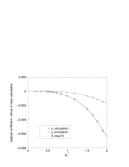
Figure 6: Simulation of the Landau mean link tadpole parameters for the Symanzik-improved action with $\chi=2$ versus self-consistent coupling $g^{2}$ with second order perturbation theory subtracted. The solid lines show fits with three loop, ${\cal O}(g_{0}^{6})$ parametrisation. For fit results see text.

IV Discussion and conclusions

Tadpole improvement via Landau mean link factors is becoming increasingly important in lattice field theory, but there are computational costs in tuning the mean-link factors to their self–consistent values. In some cases, such as the small pure gauge theory lattices used in this work, the costs are bearable. In other cases they become significant. For example, highly anisotropic lattices, such as would be used for finite temperature studies, would need to be tuned at zero temperature for a physical spatial volume. The very large time extent then required makes numerical tuning a major study in itself.

In this paper we calculate the mean link in Landau gauge perturbatively to two loop order. By comparing this to simulations, we have shown that this result predicts the mean link in Landau gauge to a high accuracy. Use of the formulae obtained remove the need for the expensive tuning.

We have used the automatic generation of the perturbative vertices to calculate the self-consistent tadpole-improvement parameters $u_{s}$, $u_{t}$ for the anisotropic Wilson and Symanzik-improved gluon action to two loops as a function of the lattice coupling $g_{0}^{2}$ and the anisotropy coefficient $\chi$. The tadpole-improved actions, Eqn. (10) are parametrised by $g_{0}$ and $\chi_{0}=\chi\,u_{s}/u_{t}$. The one and two loop coefficients are given in Tables 1 and 2, respectively, for different $\chi$. The calculation was done in Landau gauge with twisted boundary conditions in the $\mu=1,2$ directions so that there was no zero mode. Whilst the one loop and figure-of-eight integrals were done with mode summation on an $L^{4}$ lattice, the major two loop numerical Feynman integrations were done using parallel Vegas lepage78 ; numrec on an $L^{2}\times\infty^{2}$ lattice. For $L>16$ (with appropriate “squashing” of the momentum variables luwe ) there was no observable $L$-dependence. The coefficients of $g^{2}$ and $g^{4}$ for the direct perturbation series and of $g_{0}^{2}$ and $g_{0}^{4}$ for the self-consistent perturbation series are given in Tables 1–3 for different anisotropies, $\chi$. Details of the component calculations are also given in these tables to help facilitate the future calculation of different but related quantities. Interpolating fits were obtained to these coefficients as a function of $\chi$ (Table 4).

The simulation was done using a second order Langevin algorithm for the field update and the Landau gauge is fixed for each configuration using a Fourier accelerated steepest ascent method to maximise the (improved) gauge function ${\cal F}({{\hat{U}}})$.

We found that fixing to Landau gauge was very slow unless Fourier acceleration was used, and that by using twisted boundary conditions in all four directions (4–twist) the convergence of the algorithm was improved by at least a factor of ten compared with applying the twist in just two or three directions (2– or 3–twist). The reason for this is not clear but may have a connection with the suppression of tunnelling between different toron vacua, although no clear signal supporting this surmise was found. Practically, this effect was welcome in the isotropic case, and essential for $\chi=2$ where the convergence was otherwise prohibitively slow.

We did not investigate the rôle of lattice Gribov copies in fixing to Landau gauge by maximizing ${\cal F}_{L}(\{U\})$ in Eqn. (30). There has been a long discussion in the literature concerning the rôle of Gribov copies mitr:1996 ; mitr:1997 ; boea:2000 ; bock:2001 ; olsi:2001 ; olsi:2003 . In principle, the effect of selecting a local rather than the global maximum of ${\cal F}_{L}$ will be to reduce the measure values of the tadpole improvement coefficients. We believe that the effect in this calculation is negligible for a number of reasons. We do not expect a problem with Gribov copies at large-$\beta$ but some effect may occur as the physical region is approached Hart:1997ar . However, the use of twisted boundary conditions is likely to suppress the discrepancy due to the Gribov problem. This is because there is no zero-mode with such boundary conditions and by using a twist in all four directions the number of low-lying modes is reduced. In boea:2000 the effect of the zero-mode was shown to be very important in the $U(1)$ case and by performing the extra gauge transformation to remove its effect, the ZML gauge, the distribution of mean link values measured was greatly reduced. Another effect is due to double Dirac sheets (DDS) which have zero action but are strongly correlated in the $U(1)$ theory with a reduction in the mean link value and which are mooted to also be relevant in $SU(N)$ theories. We see no evidence for DDS contributions in that we see no negative spikes of the nature clearly observed in the $U(1)$ case boea:2000 . However, we have no quantitative analysis to support this remark.

If there are Gribov effects in our simulation then these will be included in the spread of results as a systematic error and are therefore to a great extent included in our quoted error which we perforce analysed by purely statistical methods Cucchieri:1997dx .

The Landau gauge function is improved; it is chosen so that it corresponds to the lattice Landau gauge used in the perturbative calculation up to term of order $g_{0}^{10}$. Thus, perturbation theory and the simulation should agree up to and including four loops.

The simulations were done on an $L^{3}\times T$ lattice with $L=8,T=16$ for the Symanzik-improved action with $\chi=2$ whch corresponds to an equal-side hypercubical lattice when measured in physical units. The couplings used were in the range $5.2\leq\beta\leq 30$. The simulation boundary conditions were twisted in all four directions, and in order to compare with calculation an adjustment for finite $L,T$ effects is needed. Finite size effects were only appreciable in the one loop coefficients. Accordingly, we used one loop coefficients calculated on a finite lattice, and two loop data for infinite volume. The higher order perturbative coefficients that are extracted may thus change slightly for larger $L$.

We fitted the data (less the two loop perturbative result) with a polynomial containing terms in $g^{4}$ and $g^{6}$. This described the data extremely well over the full range of gauge couplings. The first term in the fit function allowed for a small finite size correction to the two loop perturbative result. This finite size discrepancy corresponds to a $2\%$ correction to the two loop calculation. This is certainly very reasonable. The measurement of the three loop coefficients is accurate to $3\%$ and we should also expect a finite size error of a similar order. The main conclusion is that even in the physical region $\beta\sim 5-6$ perturbation theory works very well indeed for the Landau mean link and, moreover, there is no observable deviation from a three loop, ${\cal O}(g_{0}^{6})$ perturbative approximation. This is very encouraging for the accurate design of QCD actions and the corresponding perturbative analyses based upon them.

In principle, a full simulation analysis would give three loop numbers for a range of $\chi$ values, enabling a fit of the same form as is given in Eqn. (16). However, these coefficients are seen from the figure to be small even in the physical region, and so we conclude that $u_{s}$ and $u_{t}$ are approximated sufficiently accurately by the two loop expressions for all practical purposes.

Finally, we remark that it could be possible to calculate $u_{s}$ and $u_{t}$ by simulation using stochastic perturbation theory. However, although it has proved very successful for the expansion of the mean plaquette, the gauge fixing required here makes this approach extremely slow. Nonetheless, in general, the double expansion of the action and then the gauge potential itself as power series in the coupling required for the stochastic evolution equations is a task to which the Python code can be readily adapted.

Appendix A Twisted boundary conditions

We give here a brief description of the boundary conditions. Further details can be found in luwe ; Drummond:2002yg .

For an orthogonal twist the twisted boundary condition for gauge fields (and potentials) is

$$U_{\mu}({\mbox{\boldmath$x$}}+L_{\nu}{\mbox{\boldmath$e$}}_{\nu})=\Omega_{\nu}U_{\mu}({\mbox{\boldmath$x$}})\Omega^{-1}_{\nu}\;,$$ (50)

where the twist matrices $\Omega_{\nu}$ are constant $SU(N)$ matrices which satisfy

$$\Omega_{\mu}\Omega_{\nu}=z_{\mu\nu}\Omega_{\nu}\Omega_{\mu}$$ (51)

and $z_{\mu\nu}=\exp(2\pi in_{\mu\nu}/N)$ is an element of the centre of $SU(N)$. The particular boundary conditions imposed are uniquely specified by the antisymmetric integer tensor $n_{\mu\nu}$, $n_{\mu\nu}\in{\cal Z}_{N}$ gonzalez97 . The twisted boundary conditions can be chosen to apply in two directions only, taken here to be the (1,2) directions, but can also be applied to the 3 and 4 directions if required. Our implementation of these boundary conditions correspond to orthogonal twists since $\kappa\equiv\epsilon_{\mu\nu\sigma\rho}n_{\mu\nu}n_{\sigma\rho}=0~{}\mbox{mod}~{}N$, and consequently only configurations with integral topological charge, $Q$, will occur gonzalez97 ; the perturbation theory is then correctly associated with the $Q=0$ sector. In this case $\Omega_{3},\Omega_{4}$ can be expressed in terms of $\Omega_{1},\Omega_{2}$ once the values of $n_{\mu\nu}$ are given. We use

$$\Omega_{1}=\left(\begin{array}[]{ccc}z&0&0\\ 0&1&0\\ 0&0&z^{*}\end{array}\right)\;,~{}~{}\Omega_{2}=\left(\begin{array}[]{ccc}0&1&0\\ 0&0&1\\ 1&0&0\end{array}\right)\;,$$ (52)

The different choices of boundary condition are then given by assignments to $\Omega_{3}$ and $\Omega_{4}$ as follows:

$$\begin{array}[]{l@{~~~~}l@{~~}c}\Omega_{3}\hfil~{}~{}~{}~{}&\Omega_{4}\hfil~{}~{}&(n_{12},n_{13},n_{14},n_{23},n_{24},n_{34})\\ \hline\cr\mbox{\boldmath 1}\hfil~{}~{}~{}~{}&\mbox{\boldmath 1}\hfil~{}~{}&(1,1,0,0,0,0)\\ \Omega_{1}^{\dagger}\Omega_{2}^{\dagger}\hfil~{}~{}~{}~{}&\mbox{\boldmath 1}\hfil~{}~{}&(1,1,0,1,0,0)\\ \Omega_{1}^{\dagger}\Omega_{2}^{\dagger}\hfil~{}~{}~{}~{}&\Omega_{1}\Omega_{2}^{\dagger}\hfil~{}~{}&(1,1,1,1,1,1)\end{array}$$ (53)

We refer to these choices as 2–,3–,4–twist boundary conditions, respectively.

If the lattice has extent $L_{\mu}$ in the $\mu$–direction, the momentum spectrum is

$$k_{\mu} = \frac{2\pi\bar{k}_{\mu}}{L_{\mu}}+\frac{2\pi n_{\mu}}{NL_{\mu}}\;,~{}~{}~{}~{}\bar{k}_{\mu},n_{\mu}\in\mathbb{Z}\;,$$ (54)

$$0\leq n_{\mu}<N\;,~{}~{}~{}~{}0\leq\bar{k}_{\mu}<L_{\mu}\;.$$

For 2–twist boundary conditions, $n_{3}=n_{4}=0$. The 3–twist boundary conditions are given by $n_{3}=-(n_{1}+n_{2})$, $n_{4}=0$ and the 4–twist ones by $n_{3}=-(n_{1}+n_{2})$, $n_{4}=n_{1}-n_{2}$. In all cases we exclude the zero mode $n_{1}=n_{2}=0$.

Negative momentum in these directions is $-k_{\mu}=(-\bar{k}_{\mu},-n_{\mu})$, adding appropriate multiples of $L_{\mu}$ and $N$ respectively to remain in the ranges defined above.

Twisted boundary conditions thus replace the $N^{2}-1$ colour components of an $SU(N)$ field by a similar number of extra momentum components, interstitial to the usual reciprocal lattice. The Fourier expansion of a gauge potential is now

$$A_{\mu}(\bm{x})=\frac{1}{V_{TW}}\sum_{\bm{k}}e^{i\bm{k}\cdot\bm{x}}\Gamma({\mbox{\boldmath$n$}})\tilde{A}_{\mu}(\bm{k})\;,$$ (55)

where $V_{TW}=N\prod_{\mu}L_{\mu}$ is the twisted volume of the lattice. The sum over momentum indicates a sum over all $\bar{k}_{\mu}$ and the components of the twist vector ${\mbox{\boldmath$n$}}\equiv(n_{1},n_{2})$. The $N^{2}-1$ $SU(N)$ twist matrices are given in terms of $\Omega_{1,2}$ by

$$\Gamma({\mbox{\boldmath$n$}})=z^{(n_{1}+n_{2})(n_{1}+n_{2}-1)/2}\Omega_{1}^{-n_{2}}\Omega_{2}^{n_{1}}\;,$$ (56)

where $z=\exp(2i\pi/N)$ is an element of the centre of $SU(N)$.

We need only the trace algebra associated with these. Defining the symmetric and antisymmetric products of twist vectors

$$(\bm{n},\bm{m}) = n_{1}m_{1}+n_{2}m_{2}+(n_{1}+m_{1})(n_{2}+m_{2})\;,$$

$$\langle\bm{n},\bm{m}\rangle = n_{1}m_{2}-n_{2}m_{1}\;,$$ (57)

we obtain

$$\Gamma({\mbox{\boldmath$n$}}) = {1}~{}~{}~{}{\mbox{\boldmath$n$}}={\bf 0}~{}\mbox{mod}~{}N\;,$$

$$\mathop{\mathrm{Tr}}\left[\Gamma({\mbox{\boldmath$n$}})\right] = 0~{}~{}~{}{\mbox{\boldmath$n$}}\neq{\bf 0}~{}\mbox{mod}~{}N\;,$$

$$\Gamma({\mbox{\boldmath$n$}})^{\dagger} = z^{-{\scriptstyle{1\over 2}}({\mbox{\boldmath$\scriptstyle n$}},{\mbox{\boldmath$\scriptstyle n$}})}\Gamma(-{\mbox{\boldmath$n$}})\;,$$

$$\Gamma({\mbox{\boldmath$n$}}^{\prime})\Gamma({\mbox{\boldmath$n$}}) = z^{{\scriptstyle{1\over 2}}(\langle{\mbox{\boldmath$\scriptstyle n$}}^{\prime},{\mbox{\boldmath$\scriptstyle n$}}\rangle-({\mbox{\boldmath$\scriptstyle n$}}^{\prime},{\mbox{\boldmath$\scriptstyle n$}}))}\Gamma({\mbox{\boldmath$n$}}^{\prime}+{\mbox{\boldmath$n$}})\;,$$

$$\Rightarrow\mathop{\mathrm{Tr}}\left[\Gamma({\mbox{\boldmath$n$}}^{\prime})\Gamma({\mbox{\boldmath$n$}})\right] = Nz^{\frac{1}{2}({\mbox{\boldmath$\scriptstyle n$}},{\mbox{\boldmath$\scriptstyle n$}})}\delta_{{\mbox{\boldmath$\scriptstyle n$}},-{\mbox{\boldmath$\scriptstyle n$}}^{\prime}}\;,$$ (58)

where $({\mbox{\boldmath$n$}}~{}\mbox{mod}~{}N)$ is understood to apply to each component, $n_{1,2}$, as is the $\delta$-function. The argument of $\Gamma$ is evaluated $\mbox{mod}~{}N$.

Note that for clarity in the main text we sometimes replace the twist vectors in expressions such as Eqns. (57,58) with their associated momenta. In each case, the argument is understood to be the twist vector alone.

Note also that in Eqn. (55) the location of the gauge field, $\bm{x}$, is taken to be midway along the associated link. The components, $x_{\mu}$ are often then expressed as integer multiples of units of half a lattice spacing.