Light hadrons with improved staggered quarks: approaching the continuum limit

Abstract

We have extended our program of QCD simulations with an improved Kogut-Susskind quark action to a smaller lattice spacing, approximately 0.09 fm. Also, the simulations with $a\approx 0.12$ fm have been extended to smaller quark masses. In this paper we describe the new simulations and computations of the static quark potential and light hadron spectrum. These results give information about the remaining dependences on the lattice spacing. We examine the dependence of computed quantities on the spatial size of the lattice, on the numerical precision in the computations, and on the step size used in the numerical integrations. We examine the effects of autocorrelations in “simulation time” on the potential and spectrum. We see effects of decays, or coupling to two-meson states, in the $0^{++}$, $1^{+}$, and $0^{-}$ meson propagators, and we make a preliminary mass computation for a radially excited $0^{-}$ meson.

I Introduction

We have extended our ongoing program of lattice QCD simulations with three flavors of dynamical quarks. In this paper we describe the new simulations we have done, and present spectrum results for the light hadrons and the static quark potential. In a previous workMILC_spectrum1 we presented results for these quantities from a set of runs with a lattice spacing of approximately 0.12 fm and light quark masses ranging down to 0.2 times the estimated strange quark mass. Since that time we have extended the $a\approx 0.12$ fm runs to smaller quark masses, and increased the statistics on the $m_{u,d}=0.2\,m_{s}$ run. More importantly, we have done simulations at a smaller lattice spacing of approximately 0.09 fm in quenched QCD and with three dynamical flavors at three values of the light quark mass: $m_{u,d}=m_{s}$, $m_{u,d}=0.4\,m_{s}$ and $m_{u,d}=0.2\,m_{s}$ where $m_{s}$ is the strange quark mass estimated before doing the simulationsMILC_prelim . This enables us to address the question of lattice spacing effects, i.e., extrapolation to the continuum, to greater accuracy than we could before. Two short runs were made at larger integration step size than used in the main simulation as an additional check on the systematic errors in the simulation algorithm. At our smallest quark mass, we have computed the hadron propagators in double precision on a subset of the lattices as a check on the numerical accuracy of the computations. Finally, we have done an explicit test of the effects of the finite spatial size of the simulated system by adding a run with a larger spatial size than in the main run.

In addition to the light hadron spectrum, the gluon configurations generated in this program are being used for computations of the static quark potentialMILC_potential , heavy quark and heavy-light meson spectroscopyHEAVYQ_SPECTRUM ; FERMILAB_CHARM , heavy-light meson decay constantsHEAVYLIGHT_DECAY ; FERMILAB_CHARM , $f_{\pi}$, $f_{K}$, and chiral ${\cal O}(p^{4})$ parameters MILC_prelim ; MILC_fpi ; MILC_fpi_in-prep , $\alpha_{s}$HPQCD_alpha , exotic meson massesMILC_exotics , the topological susceptibility in QCDMILC_topology , semileptonic form factorsSEMILEPTONIC_FORM , quark massesQUARK_MASSES ; MILC_fpi ; MILC-HPQCD_MASSES , and parton distributionsPARTON_DIST . For those quantities where accurate lattice results are available and systematic errors are relatively well understood, there is good agreement with experimental values among a large set of quantitiesPRL . While this work focuses on describing the simulations, the static potential, and the light hadron spectrum, results from these other quantities are important in our analysis. In particular, the $\Upsilon$ mass splittings give the most accurate estimates of the lattice spacing, and several of these quantities enter into our estimates of the correct strange quark mass. In turn, some of the results presented here, such as the dependence of the static potential on the lattice spacing, and the tests of the effects of molecular dynamics step size and spatial size of the lattices, are important in evaluating these other works.

II Simulations

$am_{u,d}$ / $am_{s}$	$10/g^{2}$	L	$u_{0}$	res.	$\epsilon$	lats.	$a/r_{1}$
quenched	8.00	20	0.8879	na	na	408	0.3762(8)
0.02 / na	7.20	20	0.8755	$1\times 10^{-4}$	0.013	370	0.3745(14)
0.40 / 0.40	7.35	20	0.8822	$2\times 10^{-5}$	0.03	332	0.3766(10)
0.20 / 0.20	7.15	20	0.8787	$5\times 10^{-5}$	0.03	341	0.3707(10)
0.10 / 0.10	6.96	20	0.8739	$5\times 10^{-5}$	0.03	339	0.3730(14)
0.05 / 0.05	6.85	20	0.8707	$1\times 10^{-4}$	0.02	425	0.3742(15)
0.04 / 0.05	6.83	20	0.8702	$5\times 10^{-5}$	0.02	351	0.3765(14)
0.03 / 0.05	6.81	20	0.8696	$5\times 10^{-5}$	0.02	564	0.3775(12)
0.02 / 0.05	6.79	20	0.8688	$1\times 10^{-4}$	0.0133	484	0.3775(12)
$*$ 0.01 / 0.05	6.76	20	0.8677	$1\times 10^{-4}$	0.00667	658	0.3852(14)
$*$ 0.01 / 0.05	6.76	28	0.8677	$1\times 10^{-4}$	0.00667	241	0.3814(14)
$*$ 0.007 / 0.05	6.76	20	0.8678	$1\times 10^{-4}$	0.005	493	0.3783(13)
$*$ 0.005 / 0.05	6.76	24	0.8678	$5\times 10^{-5}$	0.003	197	0.3796(19)
$*$ quenched	8.40	28	0.8974	na	na	396	0.2681(5)
$*$ 0.031 / 0.031	7.18	28	0.8808	$2\times 10^{-5}$	0.02	496	0.2613(9)
$*$ 0.0124 / 0.031	7.11	28	0.8788	$5\times 10^{-5}$	0.008	527	0.2698(9)
$*$ 0.0062 / 0.031	7.09	28	0.8782	$5\times 10^{-5}$	0.004	592	0.2714(9)

Table 1: Parameters of the improved action simulations. A “*” at the beginning of the line indicates a run which is new or has been extended since the report in Ref MILC_spectrum1 . The first column gives the light and strange quark masses in lattice units, and the second column, the gauge coupling. “L” is the spatial size of the lattice. The time size is 64 for the coarse lattices and 96 for the fine lattices. $u_{0}$ is obtained from the average plaquette. The conjugate gradient residual tabulated here is the residual used in generating configurations; a smaller residual was used in computing hadron propagators. “$\epsilon$” is the time step size in configuration generation. The second to the last column is the number of stored lattices, and the last column is the lattice spacing in units of $r_{1}$ determined from the static potential in this run. A “smoothed” lattice spacing, discussed later, will be used to convert results to physical units. The last four lines, with $a\approx 0.09$ fm, will be referred to as “fine” lattices.

The simulations used here are a continuation those described in Ref. MILC_spectrum1 , which contains a more detailed description of the simulation program. We use an improved Kogut-Susskind quark action, the “$a^{2}_{\rm tad}$” or “Asqtad” action, which removes lattice artifacts up to order $a^{2}g^{2}$. Configurations were generated using the hybrid-molecular dynamics “R algorithm”R_ALGORITHM , with separate pseudofermion fields for the light and strange quarks, except where all three quarks are degenerate. The momenta conjugate to the gauge fields were refreshed at the end of every trajectory, with the trajectory length being one simulation time unit. Lattices were archived every six time units, and the hadron spectrum and static quark potential were calculated on these stored lattices.

Table 1 summarizes the parameters of the runs. For completeness, it includes runs reported in Ref. MILC_spectrum1 , although we will not repeat tabulation of masses from runs that have not been extended since that time. In identifying runs, we will quote the light (degenerate $u$ and $d$) and strange quark masses as $am_{l/s}=0.01/0.05$, for example.

III Static Potential and Length Scale

Figure 1: A “shape parameter” for the static potential, $r_{0}/r_{1}$. The red octagons are from coarse ($a\approx 0.12$ fm) lattices with three degenerate quark flavors, and the red squares from coarse lattices with two light and one strange quark. At $(M_{\pi}/M_{\rho})^{2}=0.15$ the upper square is from the $L=28$ run and the lower from the $L=20$ run. The blue crosses are from the fine ($a\approx 0.09$ fm) runs. The single green diamond is from a two flavor simulation. The magenta burst is the continuum and chiral extrapolation discussed in the text, with the smaller error bar the statistical error and the larger the systematic error. In this figure we have chosen to use $(M_{\pi}/M_{\rho})^{2}$ for the abscissa instead of the $(M_{\pi}r_{1})^{2}$ used in other figures because this lets us put the entire range of quark masses up to the quenched limit ($M_{\pi}\rightarrow\infty$) in the graph.

$am_{u,d}$ / $am_{s}$	$10/g^{2}$	$r_{1}/a$ (run)	$r_{1}/a$ (smoothed)
0.0492/0.082	6.503	1.774(10)	1.778
0.0328/0.082	6.485	1.786(10)	1.788
0.0164/0.082	6.467	1.783(12)	1.797
0.0082/0.082	6.458	1.807(10)	1.802
0.082/0.082	6.561	1.816(10)	1.805
0.0492/0.0492	6.475	1.807(28)	1.766
0.0328/0.0328	6.470	1.768(30)	1.828
0.0164/0.0164	6.430	1.796(22)	1.813
0.0492/0.0492	6.500	1.818(23)	1.821
0.0492/0.0492	6.450	1.735(30)	1.713
0.0328/0.0328	6.450	1.757(30)	1.784
0.0164/0.0164	6.450	1.857(25)	1.858
0.0082/0.0082	6.420	1.843(20)	1.827
0.005/0.050	6.76	2.634(13)	2.632
0.007/0.050	6.76	2.644(09)	2.623
0.010/0.050	6.76	2.598(08)	2.610
0.010/0.050	6.76	2.621(09)	2.610
0.020/0.050	6.79	2.649(08)	2.650
0.030/0.050	6.81	2.656(10)	2.662
0.040/0.050	6.83	2.666(11)	2.673
0.050/0.050	6.85	2.679(11)	2.683
0.030/0.030	6.79	2.678(14)	2.650
0.031/0.031	7.18	3.827(12)	3.822
0.0124/0.031	7.11	3.707(13)	3.711
0.0062/0.031	7.09	3.687(12)	3.684

Table 2: Smoothed $r_{1}/a$ compared with $r_{1}/a$ determined from each run. The top block is from lattices with $a\approx 0.18$ fm from tuning runs for our high temperature simulations, while the second and third blocks are the “coarse” and “fine” lattices respectively. Five short “tuning runs” are omitted from this table. Several of the runs have been extended since fitting of the smoothed $r_{1}$ was done.

We use the static quark potential to relate the lattice spacings in our different runs. In particular, we use the quantity $r_{1}$ defined by $r_{1}^{2}F(r_{1})=1.00$. We choose $r_{1}$ because of its ease and accuracy of computation and lack of dependence on the valence quark mass. Computation of this quantity and the effects of dynamical quarks on the potential have been discussed in Refs. MILC_potential ; MILC_spectrum1 . Here we add points at smaller quark mass and, more importantly, points at a finer lattice spacing which allow a preliminary continuum extrapolation. As before, we fit to the form in Ref. UKQCD_POTFORM ,

$$V(\vec{r})=C+\sigma r-\alpha/r+\lambda\left(V_{\rm free}(\vec{r})-1/r\right)\ \ .$$ (1)

where $V_{\rm free}(\vec{r})$ is the potential calculated in free field theory, using the improved gauge action. This lattice correction term is used at distances less than $3a$.

While we expect $r_{1}/a$ to be a smooth function of the quark masses and gauge couplings, $r_{1}/a$ determined from fitting the potential in a particular run will have a statistical error, and fluctuate from its ideal (infinite statistics) value. To minimize the effects of these run-to-run fluctuations, we have fit a smoothed $r_{1}/a$ for our three flavor lattices with quark masses less than or equal to the strange quark mass. Over the range of masses and gauge couplings we have used, a simple fitting form

$$\log(r_{1}/a)=C_{00}+C_{10}\left(\frac{10}{g^{2}}-7.0\right)+C_{01}\left(2m_{u,d}+m_{s}\right)+C_{20}\left(\frac{10}{g^{2}}-7.0\right)^{2}$$ (2)

gives an acceptable fit with a $\chi^{2}$ of 30.3 with 26 degrees of freedom, with

$$C_{00} = 1.2578(27)$$

$$C_{10} = 0.9371(93)$$

$$C_{01} = -0.828(29)$$

$$C_{20} = -0.271(22)$$ (3)

Table 2 shows values of $r_{1}/a$ used in the fit together with the smoothed $r_{1}/a$ for each run. We have used this smoothed $r_{1}/a$ in converting results from units of the lattice spacing into units of $r_{1}$.

The shape of the static quark potential is affected by dynamical quarks. One of many possible ratios parameterizing this shape is the ratio $r_{0}/r_{1}$. We use the results in Fig. 1 to extrapolate $r_{0}/r_{1}$ to the physical quark mass and continuum limit. Simultaneously fitting coarse and fine lattice results to a constant plus linear terms in the quark mass and $a^{2}\,\alpha_{s}$ gives

$$r_{0}/r_{1}=1.476(7)-0.049(10)(M_{\pi}/M_{\rho})^{2}-0.12(4)(a/r_{1})^{2}\,\alpha_{s}(a)/\alpha_{s}(0.12{\rm fm})\ \ \ ,$$ (4)

with $\chi^{2}=3.6$ for 8 degrees of freedom, using $\alpha_{s}$ from Ref. HPQCD_alpha . In fitting the potential the same distance range, $\sqrt{2}-6$, was used for all the coarse lattices, and range $\sqrt{5}-7$ for all the fine lattices. Therefore, the statistical error bars in Table 2 and Fig. 1 appropriately represent the fluctuations in $r_{1}/a$ or $r_{0}/r_{1}$ within each of these two sets of runs. However, there is a systematic effect from the choice of fit range which is common to all coarse runs and all fine runs, but may differ between the two sets. Varying the fitting range over reasonable ranges suggests that this systematic error can be conservatively estimated as an uncertainty of 0.01 in the difference between the coarse and fine lattice $r_{0}/r_{1}$. This leads to a systematic uncertainty of about 0.018 in the continuum extrapolation, leading to an estimate

$$r_{0}/r_{1}=1.474(7)(18)$$ (5)

at the physical $M_{\pi}/M_{\rho}$ in the continuum limit.

To compute $r_{1}$ in physical units, we need to set the lattice scale using a directly measurable physical quantity. A convenient choice is the $\Upsilon$ spectrum, in particular the 2S–1S and 1P–1S splittings. This gives a scale $a^{-1}=1.588(19)$ GeV on the coarse $0.01/0.05$ lattices, and $a^{-1}=2.271(28)$ GeV on the fine $0.0062/0.031$ lattices HPQCD_private . For light quark masses $\raise 1.29167pt\hbox{$<$\kern-7.5pt\lower 4.30554pt\hbox{$\sim$}}m_{s}/2$, the mass dependence of these quantities and of $r_{1}$ appears to be slight, and we neglect it. With our smoothed values of $r_{1}/a$, we then get $r_{1}=0.324(4)$ fm on the coarse lattices and $r_{1}=0.320(4)$ fm on the fine lattices.

To extrapolate $r_{1}$ to the continuum, we first assume that the dominant discretization errors go like $\alpha_{S}a^{2}$. Using $\alpha_{V}(q^{*})$ HPQCD_alpha ; LEPAGE_MACKENZIE (with scale $q^{*}=3.33/a$) for $\alpha_{S}$ gives a ratio $(\alpha_{S}a^{2})_{\rm fine}/(\alpha_{S}a^{2})_{\rm coarse}=0.428$. Extrapolating away the discretization errors linearly then results in $r_{1}=0.317(7)$ fm in the continuum. However, taste-violating effects, while formally ${\cal O}(\alpha^{2}_{S}a^{2})$ and hence subleading, are known to be at least as important as the leading errors in some cases. Therefore, one should check if the result changes when the errors are assumed to go like $\alpha^{2}_{S}a^{2}$. Taking $\alpha_{S}=\alpha_{V}(3.33/a)$ gives a ratio $(\alpha^{2}_{S}a^{2})_{\rm fine}/(\alpha^{2}_{S}a^{2})_{\rm coarse}=0.375$; while a direct lattice measurement of the taste-splittings to be presented in the next section gives a ratio of $0.35$. Extrapolating linearly to the continuum then implies $r_{1}=0.318(7)$ fm or $r_{1}=0.319(6)$ fm respectively, in agreement with the previous result. For our final result, we use an “average” ratio of 0.4 and add the effect of varying this ratio in quadrature with the statistical error. We obtain $r_{1}=0.317(7)(3)$ fm. The second error is a crude estimate of the systematic error from the choice of fit ranges for the static potential.

A similar calculation to estimate $r_{0}$ yields $0.471(6)$ fm on the coarse run and $0.466(6)$ fm on the fine run, with a continuum extrapolated value of $0.462(11)(4)$ fm, where the second error is an estimate of the systematic error from choice of fit ranges in the potential. If we take the above estimate of $r_{0}/r_{1}$ and multiply by $r_{1}=0.317$ fm, we obtain instead $r_{0}=0.467$ fm, and the difference in these two calculations of $r_{0}$ is another measure of systematic error.

IV Light Hadron Masses

Our procedures for calculating and fitting hadron propagators are described in Ref. MILC_spectrum1 . With the exception of the non-Goldstone pions at $am_{u,d}=0.0124$, we used Coulomb gauge wall sources, with eight source time slices evenly spread through the lattice. Propagators were fit with varying minimum distances, and with the maximum distance either at the midpoint of the lattice or where the fractional statistical errors exceeded 30% for two successive time slices. In most cases, to reduce the effect of autocorrelations, propagators from four successive lattices (24 simulation time units) were blocked together before computing the covariance matrix. Masses were selected by looking for a combination of a “plateau” in the mass as a function of minimum distance and a good confidence level ($\chi^{2}$) for the fit. We also made an effort to choose minimum distances that are smooth functions of the couplings, recognizing that statistically we should have some fits with low and high confidence levels.

IV.1 Pseudoscalar mesons

We calculated masses for the exact Goldstone ($\gamma_{5}\otimes\gamma_{5}$) pseudoscalar mesons in all of the runs. For the $am_{l/s}=0.0124/0.031$ run we calculated the masses of all of the different taste pions, allowing us to see how the taste symmetry breaking decreases with lattice size. Figure 2 shows the fitted masses for the pion, the kaon and the “unmixed $s\bar{s}$” from the fine lattice run with $m_{u,d}=0.2\,m_{s}$. Table 3 shows the selected fits for the pseudoscalar meson masses.

Figure 2: Pseudoscalar masses as a function of minimum distance included in the fit from the run with $10/g^{2}=7.09$ and $am_{l/s}=0.0062/0.031$. The size of the symbols is proportional to the confidence level of the fit, with the size of the symbols in the labels corresponding to 50%. These fits included only a single exponential. Fits selected to quote in the mass tables are marked with arrows.

$am_{valence}$	$am_{sea}$	$am_{PS}$	range	$\chi^{2}/D$	conf.
0.015 ($\pi$)	$\infty$	0.21643(14)	18–47	25/28	0.62
0.03 ($\pi$)	$\infty$	0.30259(14)	24–47	21/22	0.53
0.01 ($\pi$)	0.01/0.05	0.22439(20)	19–31	9.1/11	0.61
0.01 ($\pi$)	0.01/0.05	0.22421(12)	19–31	4.7/11	0.94
0.007 ($\pi$)	0.007/0.05	0.18881(19)	20–31	14/10	0.18
0.005 ($\pi$)	0.005/0.05	0.15970(20)	22–31	11/8	0.19
0.01/0.05 ($K$)	0.01/0.05	0.38327(22)	17–32	23/14	0.067
0.01/0.05 ($K$)	0.01/0.05	0.38304(20)	17–32	14/13	0.38
0.007/0.05 ($K$)	0.007/0.05	0.37268(25)	20–31	8.6/10	0.57
0.005/0.05 ($K$)	0.005/0.05	0.36550(29)	20–31	6.4/10	0.78
0.05 ($s\bar{s}$)	0.01/0.05	0.49427(18)	17–32	19/14	0.18
0.05 ($s\bar{s}$)	0.01/0.05	0.49443(18)	17–31	17/13	0.20
0.05 ($s\bar{s}$)	0.007/0.05	0.49317(19)	20–31	12/10	0.31
0.05 ($s\bar{s}$)	0.005/0.05	0.49276(23)	20–31	5.2/10	0.87
0.031 ($\pi$)	0.031/0.031	0.32003(18)	25–47	20/21	0.52
0.0124 ($\pi$)	0.0124/0.031	0.20638(18)	30–47	22/16	0.15
0.0062 ($\pi$)	0.0062/0.031	0.14794(19)	35–47	7/11	0.8
0.0124/0.031 ($K$)	0.0124/0.031	0.27209(18)	30–47	23/16	0.11
0.0062/0.031 ($K$)	0.0062/0.031	0.25319(19)	30–47	14/16	0.61
0.031 ($s\bar{s}$)	0.0124/0.031	0.32585(17)	27–47	29/19	0.07
0.031 ($s\bar{s}$)	0.0062/0.031	0.32727(14)	32–47	5.6/14	0.97

Table 3: Pseudoscalar meson masses. Here we include runs that are new or have been extended since Ref. MILC_spectrum1 ; results at larger quark masses can be found there. The first column is the valence quark mass(es), and the second column the sea quark mass or masses. The particle name is in the first column. Here “$\pi$” indicates valence quark mass equal to the lighter dynamical quarks, or degenerate in the quenched case. “$K$” indicates one valence quark equal to the light dynamical quarks and one at about $m_{s}$, while “$s\bar{s}$” indicates a fictitious meson with two valence quarks with mass about $m_{s}$, in a flavor nonsinglet state. The remaining columns are the hadron mass, the time range for the chosen fit, $\chi^{2}$ and number of degrees of freedom for the fit, and the confidence level of the fit. The first block is from the quenched run at $10/g^{2}=8.4$, the second block from the coarse three flavor runs, and the last block from the fine three flavor runs. The two lines with $am_{sea}=0.01/0.05$ are from the runs with $L=20$ and $28$.

With Kogut-Susskind quarks there are four “tastes” of valence quark, and hence sixteen different tastes of pseudoscalar mesons, grouped in eight multiplets. In the continuum limit these are degenerate, and the improved action reduces these splittings relative to the one-link fermion action. In our previous work on the coarse lattices we verified that these pion masses show the partial taste symmetry restoration predicted by Lee and SharpePARTIAL_FLAVOR_SYM . In particular, we expect near degeneracy between pairs of pions between which $\gamma_{0}$ is replaced by $\gamma_{i}$, e.g. taste $\gamma_{0}\gamma_{5}$ with taste $\gamma_{i}\gamma_{5}$. Also, the squared masses are approximately linear in the quark mass, with all tastes having the same slope. This means that a dimensionless measure of taste symmetry breaking, $\left(M_{\pi}^{2}-M_{G}^{2}\right)r_{1}^{2}$, is almost independent of the quark mass. Having verified these properties on the coarse lattice, we computed non-pointlike pion propagators on only one of the fine lattice runs, with $10/g^{2}=7.11$ and $am_{l/s}=0.0124/0.031$, which has a lattice spacing of $a/r_{1}=0.269$. In Table 4 we give these pion masses, together with those from the coarse lattice run with comparable quark masses. To facilitate comparison, these masses are given in units of $r_{1}$. We also give the measure of taste symmetry breaking, $\left(M_{\pi}^{2}-M_{G}^{2}\right)r_{1}^{2}$, for these masses. It can be seen that $\left(M_{\pi}^{2}-M_{G}^{2}\right)r_{1}^{2}$ for each taste on the fine lattices is consistently about 0.35 times the value on the coarse lattices. This is consistent with the expected scaling as $a^{2}\alpha_{S}^{2}$ described above, which, using $\alpha_{s}=\alpha_{V}(q^{*})$ and $q^{*}=3.33/a$ HPQCD_alpha suggests a ratio of 0.375.

pion taste	$M_{\pi}r_{1}$ (coarse)	$\left(M_{\pi}^{2}-M_{G}^{2}\right)r_{1}^{2}$ (coarse)	$M_{\pi}r_{1}$ (fine)	$\left(M_{\pi}^{2}-M_{G}^{2}\right)r_{1}^{2}$ (fine)	ratio
$\gamma_{5}$	0.8251(45)	-	0.7659(7)	-	-
$\gamma_{0}\gamma_{5}$	0.9386(19)	0.2003(35)	0.8127(11)	0.0739(18)	0.369(11)
$\gamma_{i}\gamma_{5}$	0.9426(16)	0.2078(30)	0.8116(26)	0.0721(42)	0.347(21)
$\gamma_{i}\gamma_{j}$	1.0033(34)	0.3259(69)	0.8372(41)	0.1143(68)	0.351(22)
$\gamma_{i}\gamma_{0}$	1.0044(29)	0.3280(59)	0.8383(26)	0.1162(44)	0.354(15)
$\gamma_{i}$	1.0555(53)	0.4334(12)	0.8576(56)	0.1489(95)	0.344(22)
$\gamma_{0}$	1.0558(32)	0.4339(67)	0.8602(37)	0.1534(64)	0.354(16)
${\bf 1}$	1.1029(80)	0.5358(75)	0.8899(93)	0.2054(165)	0.383(31)

Table 4: Taste symmetry violations on coarse and fine lattices. The second and fourth columns contain the masses for the different pions in units of $r_{1}$ for a coarse and fine lattice run. The coarse lattice run (from Ref.  MILC_spectrum1 ) was at $10/g^{2}=6.79$ and $am_{l/s}=0.02/0.05$, and had a lattice spacing $a/r_{1}=0.377$. The fine lattice run was at $10/g^{2}=7.11$ and $am_{l/s}=0.0124/0.031$, and had a lattice spacing $a/r_{1}=0.269$. The physical quark masses are similar, as evidenced by the similar Goldstone pion masses. The third and fifth columns are a measure of taste symmetry breaking, $\left(M_{\pi}^{2}-M_{G}^{2}\right)r_{1}^{2}$, on the coarse and fine lattices, and the final column is the ratio of this measure between the fine and coarse lattice runs.

In a separate analysis we calculate “partially quenched” pseudoscalar masses and decay constants, where the valence quark and sea quarks have different massesMILC_fpi ; MILC_fpi_in-prep . These results have been analyzed using chiral perturbation theory including terms parameterizing the taste symmetry breakingSCHPT . From this analysis we find $f_{\pi}$ and $f_{K}$ at the physical quark masses, and values for several of the low energy constants in chiral perturbation theory. Another product of the computations of $m_{PS}$ and $f_{PS}$ is a determination of the lattice quark masses corresponding to the real world. We define the strange and light quark masses at fixed lattice spacing, $am^{\rm lat}_{s}$ and $am^{\rm lat}_{u,d}$, to be the lattice masses that give the experimental values for $M_{K}$ and $M_{\pi}$. To determine $am^{\rm lat}_{s}$ and $am^{\rm lat}_{u,d}$, we fit the mass and decay constant data to chiral log forms that take into account staggered taste violations SCHPT . We find $am^{\rm lat}_{s}=0.0390(1)({}^{+18}_{-20})$, $am^{\rm lat}_{u,d}=0.00148(1)({}^{+6}_{-8})$ on the coarse lattices, and $am^{\rm lat}_{s}=0.0272(1)({}^{+12}_{-10})$, $am^{\rm lat}_{u,d}=0.00103(0)(4)$ on the fine lattices, where the errors are statistical and systematic. The systematic error is dominated by that coming from the chiral extrapolation/interpolation and the $\sim\!2\%$ scale uncertainty.

We have also calculated masses of excited pseudoscalar mesons. Because this requires consideration of two-meson states, discussion of this is deferred to a later section on hadronic decays and excited states.

IV.2 Vector mesons

Figure 3 shows vector meson masses versus minimum distance fit for the fine lattice run with the lightest quark mass. Mass estimates for all of the runs are in Table 5. Note that despite our relatively small quark masses, none of these vector mesons are below the threshold for decay into two pseudoscalars, since the angular momentum of the vector mesons requires that the vector meson at rest decay into pseudoscalars with momentum $2\pi/L$. In addition, we require a combination of tastes in the pseudoscalars that overlaps with the taste of the vector meson — the vector mesons tabulated here have spin $\otimes$ taste $=\gamma_{i}\otimes\gamma_{i}$.

Table 6 shows masses for $1^{+}$ mesons. These mesons can decay into a vector and a pseudoscalar meson, and these simulations reach into the quark mass region where this threshold is crossed. We defer discussion of this effect to the next section.

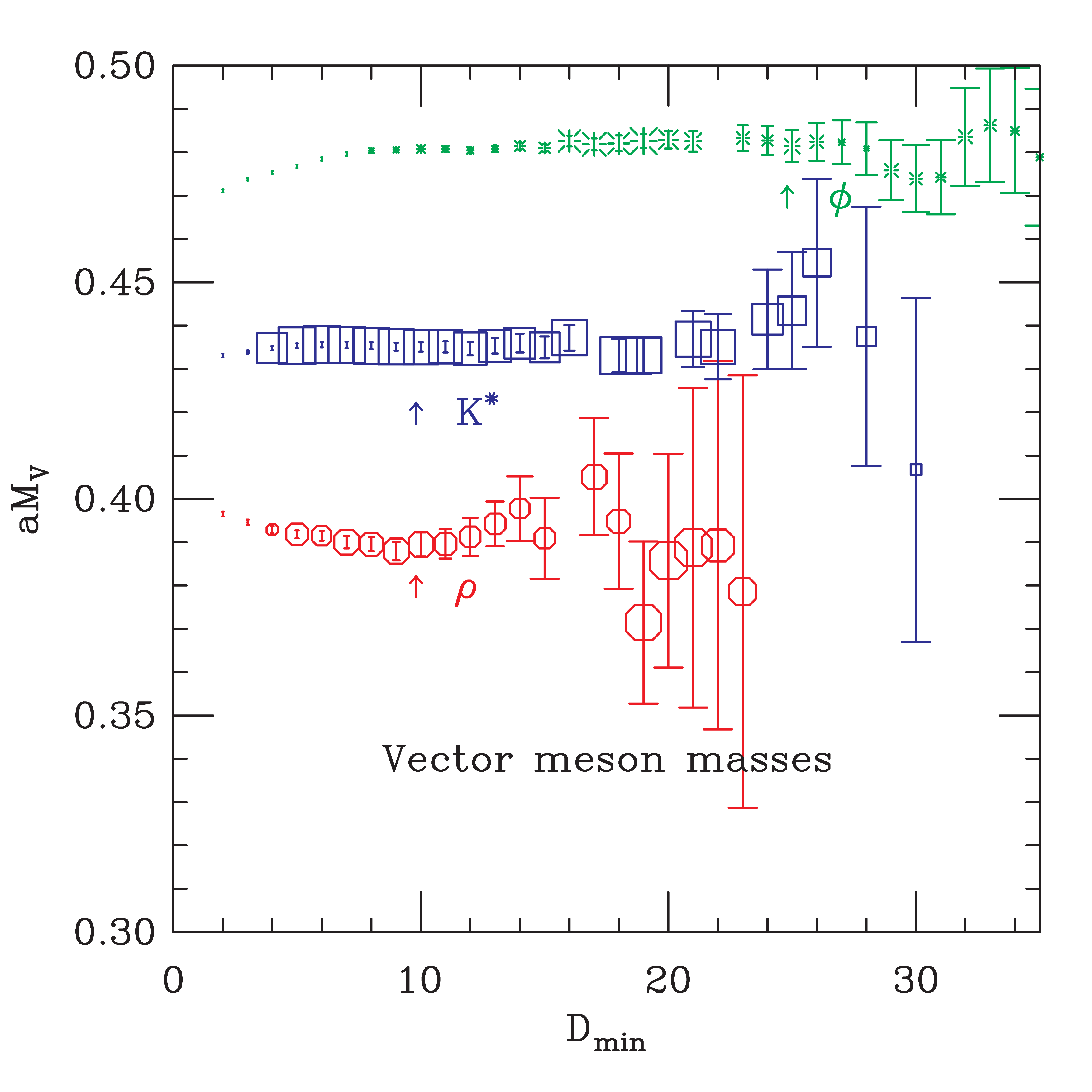
Figure 3: Vector meson masses as a function of minimum distance included in the fit from the run with $10/g^{2}=7.09$ and $am_{l/s}=0.0062/0.031$.

$am_{valence}$	$am_{sea}$	$am_{V}$	range	$\chi^{2}/D$	conf.
0.015 ($\rho$)	$\infty$	0.4660(30)	11–25	4/11	0.97
0.03 ($\rho$)	$\infty$	0.4992(15)	5–25	18/15	0.28
0.01 ($\rho$)	0.01/0.05	0.5690(50)	6–22	15/13	0.32
0.01 ($\rho$)	0.01/0.05	0.5680(30)	6–19	10/10	0.42
0.007 ($\rho$)	0.007/0.05	0.5510(40)	6–18	11/9	0.26
0.005 ($\rho$)	0.005/0.05	0.5340(80)	6–15	5.8/6	0.44
0.01/0.05 ($K^{*}$)	0.01/0.05	0.6492(25)	8–23	5.2/12	0.95
0.01/0.05 ($K^{*}$)	0.01/0.05	0.6462(18)	8–27	29/16	0.023
0.007/0.05 ($K^{*}$)	0.007/0.05	0.6330(30)	9–23	10/11	0.54
0.005/0.05 ($K^{*}$)	0.005/0.05	0.6190(40)	10–23	15/10	0.12
0.05 ($\phi$)	0.01/0.05	0.7193(14)	9–30	11/18	0.90
0.05 ($\phi$)	0.01/0.05	0.7194(11)	9–31	15/19	0.74
0.05 ($\phi$)	0.007/0.05	0.7114(16)	12–30	12/15	0.69
0.05 ($\phi$)	0.005/0.05	0.7140(30)	14–29	15/12	0.25
0.031 ($\rho$)	0.031/0.031	0.4781(14)	16–42	36/23	0.043
0.0124 ($\rho$)	0.0124/0.031	0.4173(13)	10–33	31/20	0.059
0.0062 ($\rho$)	0.0062/0.031	0.3895(28)	10–27	11/14	0.65
0.0124/0.031 ($K^{*}$)	0.0124/0.031	0.4483(18)	15–42	42/24	0.013
0.0062/0.031 ($K^{*}$)	0.0062/0.031	0.4350(11)	10–34	13/21	0.91
0.031 ($\phi$)	0.0124/0.031	0.4831(8)	14–47	55/30	0.0032
0.031 ($\phi$)	0.0062/0.031	0.4810(40)	25–45	18/17	0.39

Table 5: Vector meson masses. Runs tabulated and the format are the same as in Table 3. Here “$\rho$” indicates valence quark mass equal to the lighter dynamical quarks, or degenerate in the quenched case. “$K^{*}$” indicates one valence quark equal to the light dynamical quarks and one at about $m_{s}$, while “$\phi$” indicates two valence quarks with mass about $m_{s}$, although in a flavor nonsinglet state.

$am_{valence}$	$am_{sea}$	$am_{PV}$	range	$\chi^{2}/D$	conf.
0.015 ($a_{1}$)	$\infty$	0.720(40)	9–25	11/11	0.48
0.03 ($a_{1}$)	$\infty$	0.730(6)	7–25	10/13	0.67
0.015 ($b_{1}$)	$\infty$	0.741(22)	6–25	7.3/14	0.92
0.03 ($b_{1}$)	$\infty$	0.748(10)	7–25	15/13	0.33
0.01 ($a_{1}$)	0.01/0.05	0.820(40)	6–15	5.3/6	0.50
0.01 ($a_{1}$)	0.01/0.05	0.848(24)	6–17	6.4/8	0.60
0.007 ($a_{1}$)	0.007/0.05	0.767(21)	5–15	10/7	0.16
0.005 ($a_{1}$)	0.005/0.05	0.790(40)	5–15	9.6/7	0.21
0.01 ($b_{1}$)	0.01/0.05	1.020(90)	6–22	15/13	0.32
0.01 ($b_{1}$)	0.01/0.05	0.980(60)	6–19	10/10	0.42
0.007 ($b_{1}$)	0.007/0.05	0.810(40)	5–18	11/10	0.34
0.005 ($b_{1}$)	0.005/0.05	0.700(90)	6–15	5.8/6	0.44
0.031 ($a_{1}$)	0.031/0.031	0.667(4)	8–25	11/12	0.56
0.0124 ($a_{1}$)	0.0124/0.031	0.600(8)	8–30	22/19	0.30
0.0062 ($a_{1}$)	0.0062/0.031	0.532(19)	10–26	14/13	0.36
0.031 ($b_{1}$)	0.031/0.031	0.681(5)	7–25	21/13	0.08
0.0124 ($b_{1}$)	0.0124/0.031	0.632(9)	7–33	34/23	0.07
0.0062 ($b_{1}$)	0.0062/0.031	0.650(50)	10–27	11/14	0.65

Table 6: Pseudovector meson masses. Runs tabulated and the format are the same as in Table 3.

IV.3 Baryons

Table 7 contains masses for the octet nucleon and $\Xi$. We do not tabulate the $\Lambda$ and $\Sigma$ since our code does not cleanly separate the light quark isospins. In principle, the nucleon mass could be fit by methods similar to those used for the pion mass and decay constant, incorporating effects of continuum chiral corrections, lattice artifacts like taste symmetry breaking, finite size effects and partial quenching. Such an analysis is not yet available. However, statistical errors on the nucleon mass are much larger than for the pseudoscalars, so this full machinery may be less important here. An alternative strategy for dealing with lattice artifacts is to perform a continuum extrapolation at the quark masses used in simulations, and then fit these extrapolated masses to continuum chiral perturbation theory. Figure 4 shows the nucleon masses in units of $r_{1}$. This graph also contains a very rough sketch of how such a continuum and chiral extrapolation might begin. The right most magenta fancy plus is a linear extrapolation in $a^{2}\alpha_{s}$ of the coarse and fine results at $m_{u,d}\approx 0.4\,m_{s}$ to $a=0$, as indicated by the red line. The middle fancy plus is a similar continuum extrapolation at $m_{u,d}\approx 0.2\,m_{s}$. The solid straight line is a linear extrapolation to the physical pion mass. As a rough estimate of the effects of chiral logarithms, the two curved lines are chiral perturbation theory forms constrained to match the two continuum extrapolated points. These forms have two free parameters, so we emphasize that this is not a fit and there is no test of consistency of these forms with our data. The yellow upper curved line is an expansion in powers of $M_{\pi}$ up to order $M_{\pi}^{2}\log(M_{\pi})$ from Ref. LEINWEBER and the cyan lower curve is a form where the nucleon-delta mass splitting is also treated as smallVBERNARD . It is clear that fine lattice results at a smaller quark mass will be needed, since the slopes of the chiral perturbation theory forms are clearly different from the lattice results for quark masses as small as $0.4\,m_{s}$.

$am_{valence}$	$am_{sea}$	$am_{B}$	range	$\chi^{2}/D$	conf.
0.015 (N)	$\infty$	0.6267(18)	8–23	14/12	0.30
0.03 (N)	$\infty$	0.7134(18)	12–30	11/15	0.78
0.01 (N)	0.01/0.05	0.7710(40)	6–16	4.4/7	0.74
0.01 (N)	0.01/0.05	0.7670(30)	6–17	3.8/8	0.88
0.007 (N)	0.007/0.05	0.7480(30)	5–14	5/6	0.54
0.005 (N)	0.005/0.05	0.7230(60)	5–14	9.8/6	0.13
0.01/0.05 ($\Xi$)	0.01/0.05	0.9810(30)	8–20	5.3/9	0.81
0.01/0.05 ($\Xi$)	0.01/0.05	0.9737(20)	8–21	16/10	0.09
0.007/0.05 ($\Xi$)	0.007/0.05	0.9670(50)	10–20	9.2/7	0.24
0.005/0.05 ($\Xi$)	0.005/0.05	0.9540(80)	10–19	4.6/6	0.60
0.031 (N)	0.031/0.031	0.6996(11)	7–37	50/25	0.0023
0.0124 (N)	0.0124/0.031	0.5815(19)	10–29	17/16	0.41
0.0062 (N)	0.0062/0.031	0.5190(40)	11–23	4.6/9	0.87
0.0124/0.031 ($\Xi$)	0.0124/0.031	0.6696(17)	13–33	12/17	0.80
0.0062/0.031 ($\Xi$)	0.0062/0.031	0.6519(18)	12–30	19/15	0.21

Table 7: Octet baryon masses. Runs tabulated and the format are the same as in Table 3.

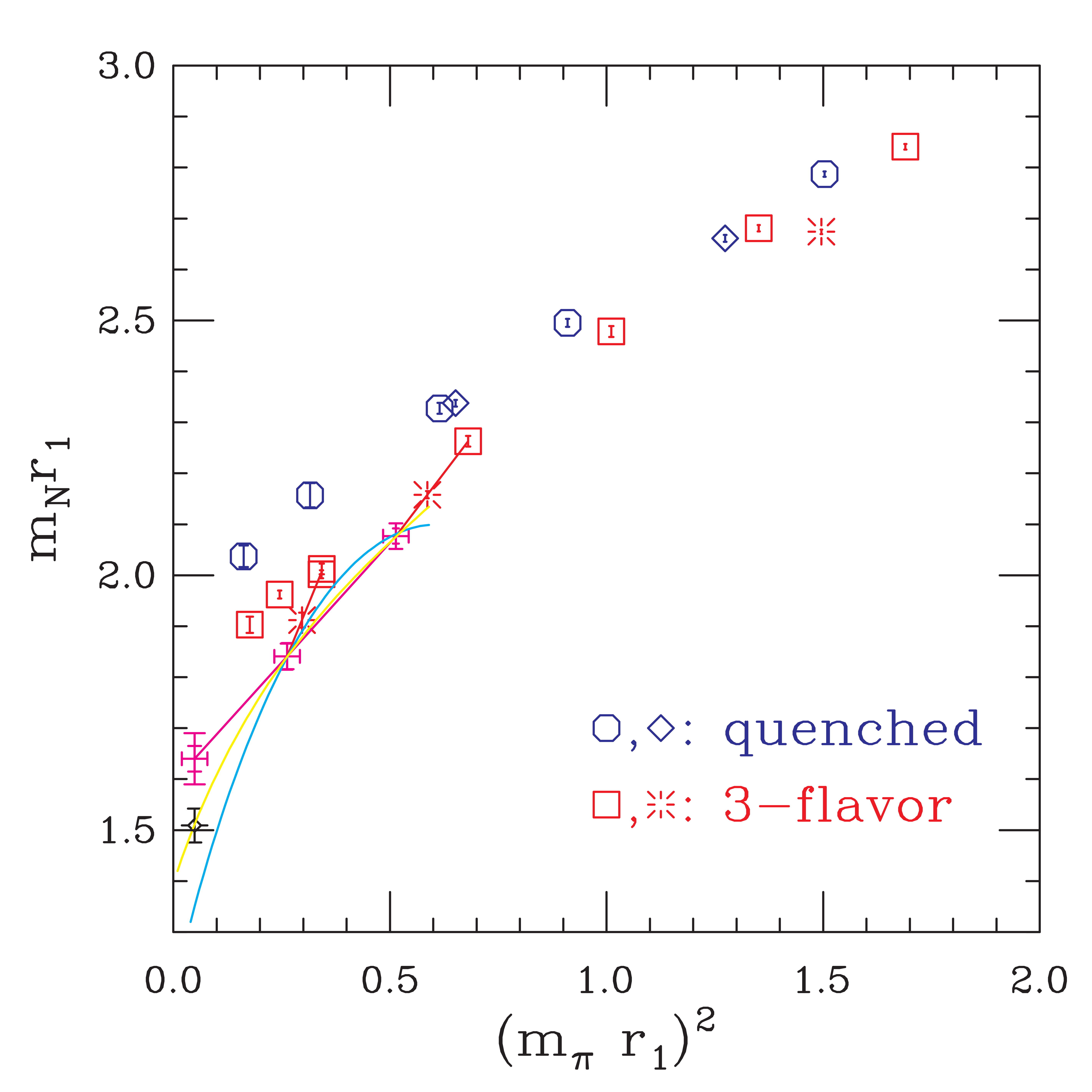
Figure 4: Nucleon masses. The blue diamonds and octagons are quenched coarse and fine runs respectively. The red squares are three flavor coarse lattice results, and the red bursts the three flavor fine lattices. The magenta fancy plusses connected by the straight line and the two curved lines are continuum and chiral extrapolations discussed in the text. The fancy diamond is the experimental value, with an error bar from the uncertainty in $r_{1}$.

V Tests of Systematic and Statistical Errors

The results in the previous two sections allow us to make several algorithm tests as well as more physical tests.

V.1 Single versus double precision

As the valence quark masses are made smaller, the condition number of the fermion matrix increases and one might worry that double precision is necessary for computing the hadron propagators. In general, we have used single precision for the computations at each lattice site, with global sums in double precision. At our smallest quark mass, $am_{u,d}=0.005$, we have tested the accuracy of our hadron spectrum and static potential computations by repeating the computation in double precision on a subset of the lattices. Table 8 shows results for a number of quantities evaluated on a set of 137 lattices with $am_{l/s}=0.005/0.050$. Note that since these are fit on exactly the same sets of lattices with exactly the same programs, any discrepancies are the result of the different precision. However, we provide statistical errors to show how the effects of roundoff compare with the statistical errors. For all of these quantities the effects of using single precision are small compared with the statistical errors, and with the statistical errors we would get from any reasonable lengthening of this run.

Quantity	Double	Single	Comment
$V(2,0,0)$	0.829883(852)	0.829888(853)	potential at r=(2,0,0)
$V(2,2,2)$	1.05426(503)	1.05451(502)
$V(3,3,3)$	1.2511(194)	1.2511(194)
$r_{1}/a$	2.63933(1679)	2.63915(1678)	t=4–5, block=5
$r_{0}/r_{1}$	1.4566(64)	1.4566(64)	t=4–5, block=5
$\pi(20)$	411.53(1.55)	411.44(1.55)	prop. at d=20
$\rho(6)$	143.76(1.78)	143.73(1.78)
$aM_{\pi}$	0.15965(22)	0.15966(21)	d=20–31, $\chi^{2}/D=0.60$
$aM_{K}$	0.36519(34)	0.36519(34)	d=20–32, $\chi^{2}/D=0.82$
$aM_{\rho}$	0.5330(83)	0.5330(83)	d=6–14, $\chi^{2}/D=0.85$
$aM_{N}$	0.7311(84)	0.7312(84)	d=6–14, $\chi^{2}/D=0.50$

Table 8: Comparison of results with single and double precision computations. The first three lines are the static quark potential at three different spatial separations. These separations are in the spatial region used in fitting the potential. The next two lines are parameters extracted from fitting the potential, the inverse lattice spacing in units of $r_{1}$ and a “shape parameter” $r_{0}/r_{1}$. The second part of the table contains hadron propagator comparisons. The $\pi(20)$ and $\rho(6)$ show the pion and rho propagators summed over a time slice at time separations 20 and 6. These distances are near the minimum of the range used in fitting the masses, and so are among the most important distances in our fits. Finally, the last four lines are hadron masses computed from the double and single precision propagators.

V.2 Integration step size

Our simulation algorithm is expected to introduce errors proportional to $\epsilon^{2}$ where $\epsilon$ is the simulation time step size. Based on previous experience and our expectations about the scaling of the fermion force with the quark mass, we have used a step size of about 2/3 of the light quark mass in these runs. As a check on these effects, we have made short runs with larger step sizes at one of our small quark masses (the same parameters at which we checked effects of the spatial size of the lattice.) The production runs here were done at a step size of $\epsilon=0.0067$ (658 lattices), and the short tests at step sizes of $0.01$ (49 lattices) and $0.01333$ (53 lattices) with lattice size $20^{3}\times 64$. Table 9 shows results for the static quark potential and some hadron masses at these different step sizes, using the same fitting ranges in each case. Since the short runs were too short for a good error analysis, statistical errors on these quantities are estimated by scaling the errors on the $L=20$, $\epsilon=0.0067$ run by the square root of the ratio of the numbers of configurations used.

	$L=20$	$L=28$	$L=20$	$L=20$
Q.	$\epsilon=0.0067$	$\epsilon=0.0067$	$\epsilon=0.0100$	$\epsilon=0.013$
$\Box$	1.70092(2)	1.70094(3)	1.70096(7)	1.70066(7)
$\bar{\psi}\psi$	0.07421(10)	0.07420(13)	0.07374(37)	0.07488(35)
$r_{1}/a$	2.598(8)	2.621(9)	2.649(29)	2.619(28)
$aM_{\pi}$	0.22439(20)	0.22421(12)	0.22500(73)	0.22554(70)
$aM_{\rho}$	0.569(5)	0.568(3)	0.557(18)	0.558(18)
$aM_{N}$	0.771(4)	0.767(3)	0.785(15)	0.753(14)

Table 9: Effect of integration step size. These are from runs with $10/g^{2}=6.76$ and $am_{l/s}=0.01/0.05$. Columns two and three are our long runs with $L=20$ and $28$ using a step size of $0.0067$. (Our usual practice is to use a step size about 2/3 of the lightest quark mass.) Columns four and five are from short runs with step sizes $0.01$ and $0.01333$.

V.3 Spatial size of the lattice

In one of our coarse lattice runs, $10/g^{2}=6.76$, $am_{l/s}=0.01/0.05$, we have made a second run at a larger spatial lattice size, $28^{3}\times 64$. (We have also lengthened the run with $L=20$, so this is the run where we have the best statistics.) This allows us to explicitly check the effects of the spatial lattice size. Table 10 shows the results of this test for the static quark potential and simple hadron propagators. Note that these values of $r_{1}/a$ fall on opposite sides of the interpolated (“smoothed $r_{1}$”) value of 2.610, and the values of $r_{0}/r_{1}$ fall on opposite sides of a straight line fit to the coarse lattice points in Fig. 1, leading us to believe that we do not see any statistically significant finite size effects in either the potential or the hadron masses. The sizes of these two lattices in physical units are 2.43 and 3.40 fm, using $r_{1}=0.317$ fm to set the scale, and $M_{\pi}L$ is 4.48 and 6.27 respectively. Using the (staggered) chiral fits MILC_fpi ; MILC_fpi_in-prep to light pseudoscalar masses and decay constants, it is possible to estimate the leading finite volume correction on $M_{\pi}$. We expect a difference $\Delta=0.00026$ between $L=20$ and $L=28$ results, consistent with the observed value in the simulations, $\Delta=0.00018(23)$, shown in Table 10.

Quantity	$L=20$	$L=28$	$\Delta$
$r_{1}/a$	2.598(8)	2.621(9)	-0.023(12)
$r_{0}/r_{1}$	1.4461(36)	1.4533(34)	-0.0072(50)
$M_{\pi}$	0.22439(20)	0.22421(12)	0.00018(23)
$M_{\rho}$	0.569(5)	0.568(3)	0.001(6)
$M_{N}$	0.771(4)	0.767(3)	0.004(5)

Table 10: Comparison of results with different spatial sizes. These are from the runs with $10/g^{2}=6.76$ and $am_{l/s}=0.01/0.05$. The spatial sizes were $L=20$ and $28$, corresponding to physical sizes of $2.4$ and $3.4$ fm, using $r_{1}=0.317$ fm to set the physical scale. The first two lines are parameters extracted from fitting the potential, the inverse lattice spacing in units of $r_{1}$ and a “shape parameter” $r_{0}/r_{1}$. The second part of the table contains hadron mass comparisons. $\Delta$ is the $L=20$ value minus the $L=28$ value in each row.

V.4 Autocorrelations

Because of the high cost of generating sample configurations with dynamical quarks, successive samples were taken at simulation time intervals such that they are not completely statistically independent. The resulting autocorrelations (in simulation time) affect the statistical errors on all of the computed quantities. The “exponential autocorrelation time”, which is determined by the eigenvalue of the Markov process matrix which is closest to one, is expected to be the same for all calculated quantities. However, the contribution of this slowest mode to various quantities varies, and to parameterize the effect of autocorrelations on individual quantities we use the “integrated autocorrelation time”, $\tau_{\rm int}=\sum_{s}C_{Q}(s)$, where $s$ runs over the simulation time separations and $C_{Q}(s)$ is the normalized autocorrelation for quantity $Q$,

$$C_{Q}(s)=\frac{\langle Q(t+s)Q(t)\rangle-\langle Q\rangle^{2}}{\langle Q(t)Q(t)\rangle-\langle Q\rangle^{2}}\ \ \ .$$ (6)

Because we need a covariance matrix to calculate masses from the average propagators, and getting a nonsingular covariance matrix requires more samples than there are points in the fit range, we cannot get a hadron mass from one sample. So, to study autocorrelations of hadron mass estimates we use the “mirror image” of this procedure — we do single elimination jackknife fits with one sample omitted from the data set and compute the autocorrelations of these jackknife fits. Figure 5 shows the jackknife pion masses as a function of the simulation time of the omitted sample for the run with $10/g^{2}=6.76$ and $am_{l/s}=0.01/0.05$. For example, Table 11 shows $C_{Q}(6)$ where $Q$ is the $\pi$, $\rho$ or nucleon mass or the amplitude in the pion propagator, and the simulation time separation is six units, corresponding to successive stored lattices. From this table we can see that the normalized autocorrelation is largest for the pion mass, and has no obvious systematic dependence on the light quark mass. Therefore, we average the autocorrelations over the quark masses, separately for the coarse and fine runs. The resulting autocorrelations as a function of simulation time separation are plotted in Fig. 6.

Not surprisingly, the autocorrelation times are larger on the fine lattices than on the coarse lattices. In Ref. MILC_topology autocorrelations of the topological charge were computed on these lattices. The topological charge evolves more slowly than the hadron masses, with estimated autocorrelation times as large as 35 time units for the $10/g^{2}=7.18$, $am_{l/s}=0.031/0.031$ run. We refer the reader to MILC_topology for more discussion.

$10/g^{2}$	$am_{u,d}$	N	$M_{\pi}$	$A_{\pi}$	$M_{\rho}$	$M_{N}$
6.85	0.05	425	0.196	0.079	0.047	0.077
6.83	0.04/0.05	351	0.383	0.127	-0.031	0.119
6.91	0.03/0.05	564	0.274	0.161	0.082	0.070
6.79	0.02/0.05	486	0.173	0.169	0.025	0.143
6.76	0.01/0.05	658	0.229	0.056	0.046	0.014
6.76	0.007/0.05	487	0.150	0.056	-0.055	-0.020
	average	2971	0.229	0.106	0.024	0.062
7.18	0.031	496	0.426	0.223	0.074	0.203
7.11	0.0124/0.031	534	0.311	0.142	-0.002	0.034
7.09	0.0062/0.031	586	0.283	0.152	0.055	0.011
	average	1616	0.336	0.170	0.042	0.078

Table 11: Normalized autocorrelations $C_{Q}(6)$ for hadron masses and the pion amplitude in the light quark runs. The third column is the number of samples in each run. We also show the results averaged over all the coarse runs, and over all the fine runs, where the third column is the total number of coarse or fine lattices.

Figure 5: Single elimination jackknife masses for the pion, from the run with $10/g^{2}=6.76$ and $am_{l/s}=0.01/0.05$, using fits with $D_{\rm min}=19$.

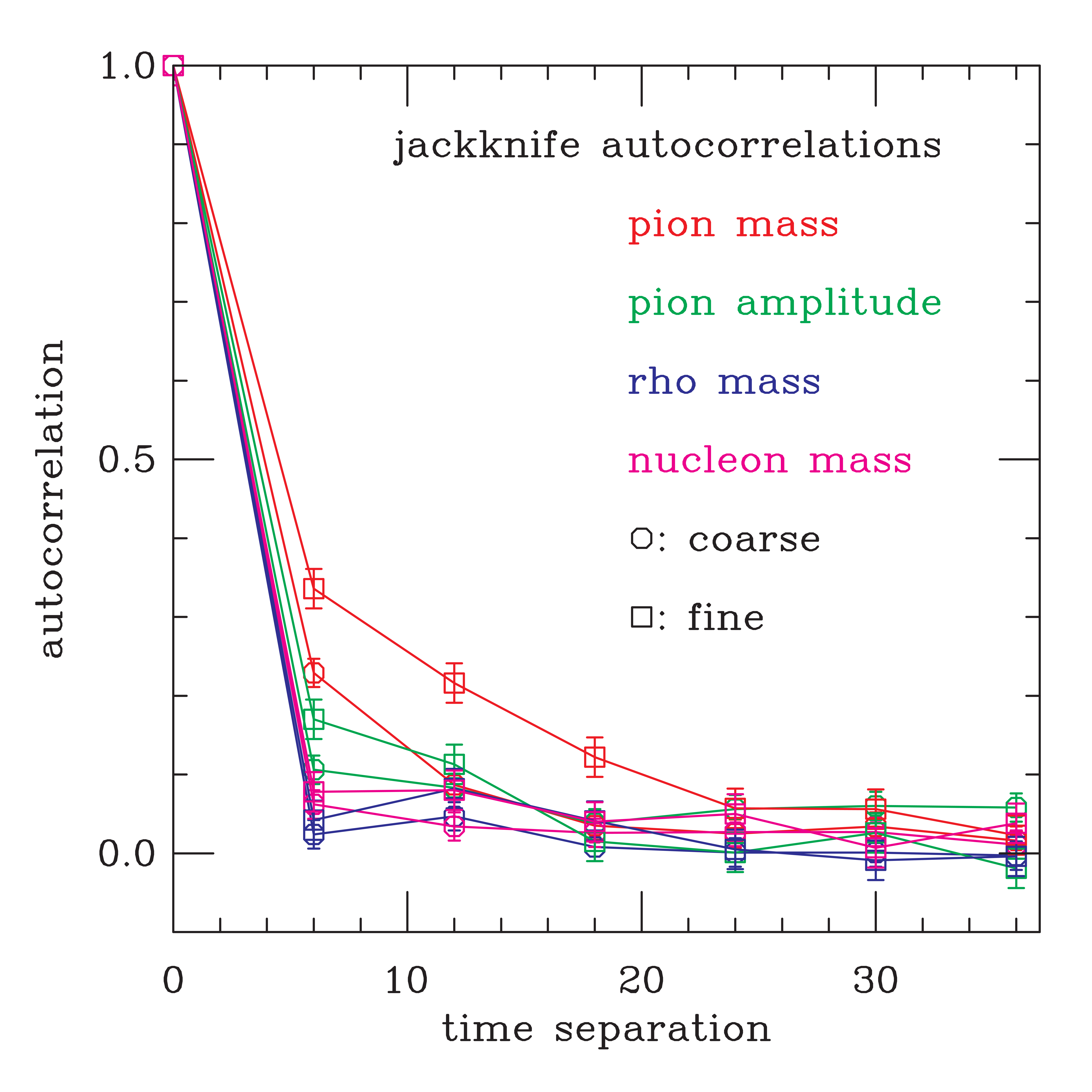
Figure 6: Normalized autocorrelations for the $\pi$, $\rho$ and nucleon masses and the amplitude of the pion propagator as functions of the separation in simulation time. Results for all the coarse lattice runs are averaged together, as are all the fine lattice runs.

VI Hadronic decays and excited states

When the quark mass is small enough, most of the hadrons we study are unstable, decaying strongly into two or more lighter hadrons. In principle, although not always in practice, fitting to the ground state mass in our propagators will give the mass of the lightest state with the right quantum numbers in the periodic box, which in many cases will be a two particle state. In Ref. MILC_spectrum1 we showed this effect in the $0^{++}$ ($a_{0}$) channel. Figure 7 updates this plot with more results on coarse lattices at light quark mass, and the new results on the fine lattices. For the three flavor runs, the fine lattice points agree well with the coarse lattice results. The figure also shows the mass of the lowest energy two-meson state expected to couple to this particle, $\pi+\eta$. Surprisingly, the new points at the lighest quark masses increasingly deviate from this two-meson mass, which is not understood. The light mass quenched propagators remain difficult to fit, which may not be surprising for unstable particles in an unphysical theory. We have not yet tried fitting to the particle-plus-ghost form suggested by Bardeen et al. Bardeen:2001jm . For quark masses where the two-meson state has lower energy, it would be satisfying to find a one meson ($a_{0}$) state as an excited state in the propagator. Our attempts to do this have been unsuccessful so far. In the fine lattice run at $am_{l/s}=0.0062/0.031$ we were able to extract an excited state mass, shown as the cyan decorated square in Fig. 7. However, the mass of this state is still much smaller than the extrapolations from large quark mass, and it is likely also a two-meson state, perhaps $K\bar{K}$.

We also expect to see the pseudovector ($1^{+}$) mesons couple to two zero-momentum mesons, although for these mesons we are not as far below the threshold as in the $0^{++}$ case. Figure 8 shows $1^{+-}$ ($b_{1}$) masses as a function of quark mass along with the decay channel mass $M_{\rho}+M_{\pi}$. We tentatively attribute the downturn at the lightest quark masses to this decay, although better statistics at the lightest coarse lattice and a lighter mass fine lattice run would clarify the situation. Again, we are unable to get good fits for the lightest mass quenched propagators.

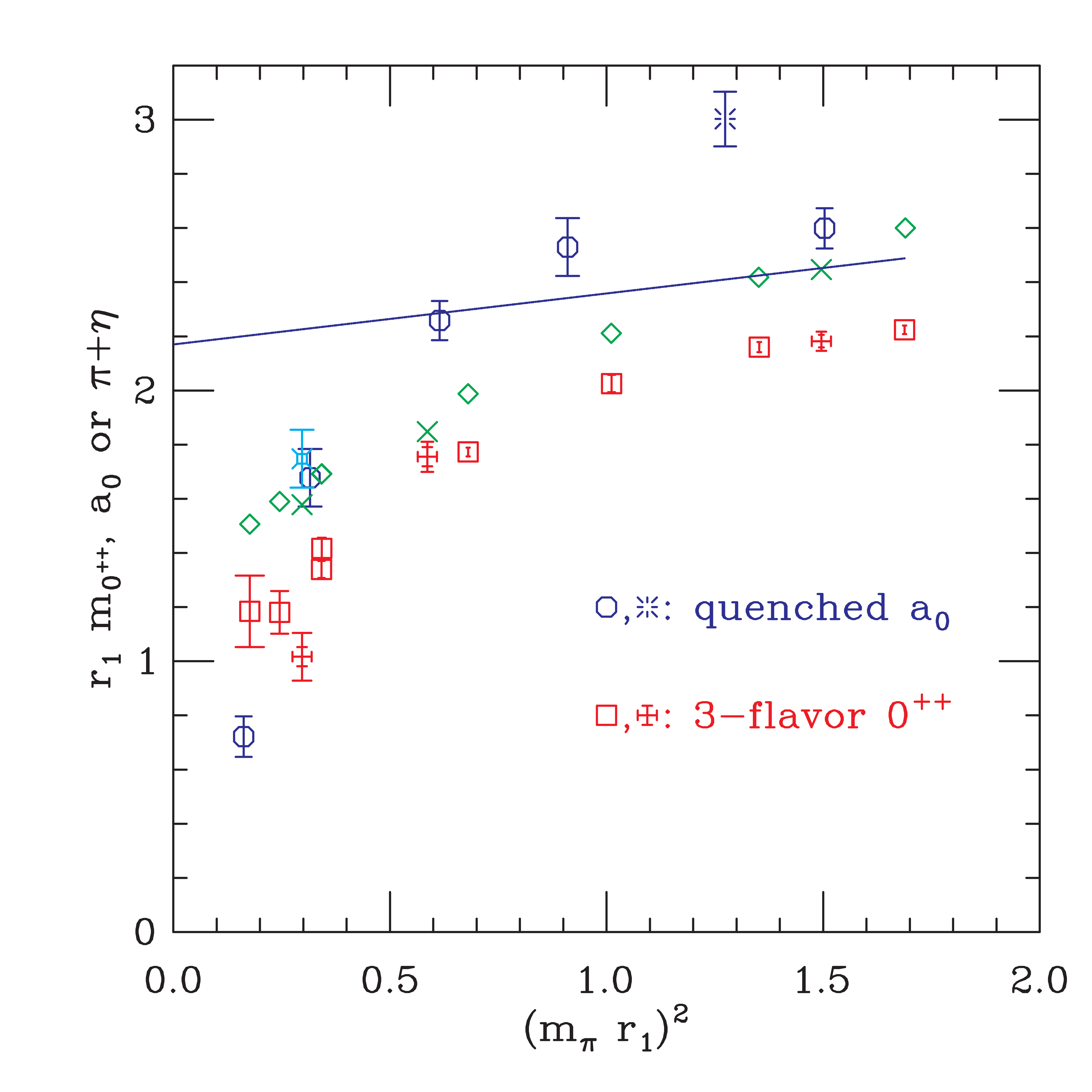
Figure 7: $0^{++}$ energies. The red squares are three flavor coarse runs, and the red fancy plusses, three flavor fine runs. The blue octagons are a quenched coarse run and the blue burst a quenched fine run. The cyan decorated square is an excited $0^{++}$ mass from one of the runs. The green diamonds and crosses are sums of $\pi$ and $\eta$ masses on coarse and fine runs respectively, where the $\eta$ mass is estimated from $M_{\eta}^{2}=\frac{1}{3}M_{\pi}^{2}+\frac{2}{3}m_{s\bar{s}}^{2}$, with $m_{s\bar{s}}$ the unmixed $s\bar{s}$ pseudoscalar mass. The straight blue line is an extrapolation of $a_{0}$ masses from heavier quark runs (not shown in this graph).

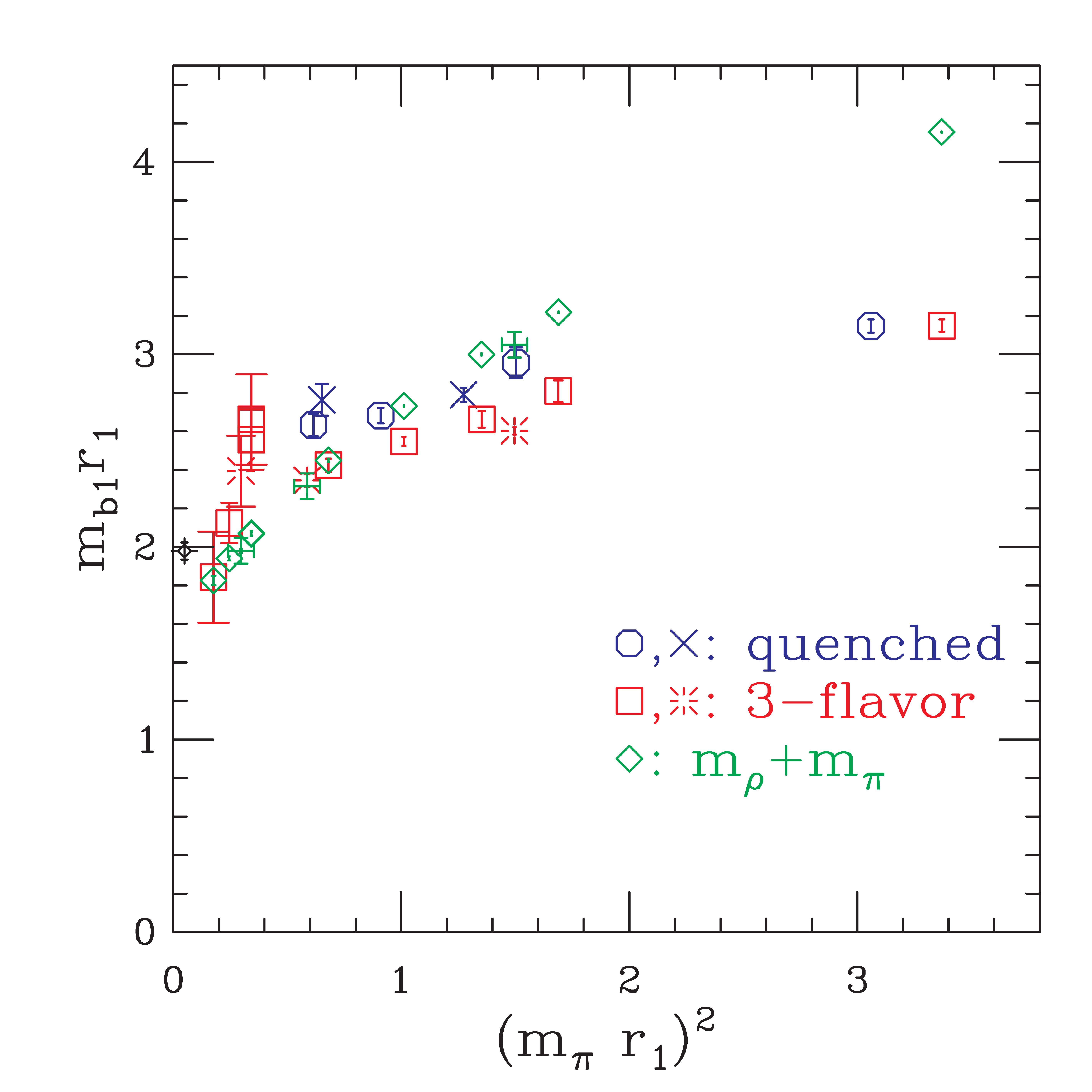
Figure 8: $1^{+-}$ energies. The red squares are three flavor coarse runs and the red bursts three flavor fine runs. The blue octagons and crosses are quenched coarse and fine runs respectively. The green diamonds and fancy plusses are sums of rho and pion masses on coarse and fine three flavor runs respectively. The fancy diamond on the left is the experimental value, with an error bar corresponding to the uncertainty in $r_{1}$.

Kogut-Susskind meson propagators generally include normal exponential contributions from one $J^{PC}$ value and an oscillating exponential component from a parity partner state. In the case of the Goldstone pion, the parity partner has the exotic $J^{PC}=0^{+-}$ and thus does not contribute to the propagator. In combination with a relatively high signal-to-noise ratio at all time separations, this enhances our ability to determine the $0^{-+}$ contributions. Specifically, in addition to the one-state fits, which we presented in Figure 2 and Table 3, when we performed a two-state fit of the pseudoscalar propagator data, we were able to determine the mass of a second, excited $0^{-+}$ state. We have presented preliminary results of this analysis in MILC_excited . We fit $0^{-+}$ propagators to the form:

$$C(t)=A_{0}(e^{-M_{0}t}+e^{-M_{0}(T-t)})+A_{1}(e^{-M_{1}t}+e^{-M_{1}(T-t)}),$$ (7)

where $A_{0}$ and $M_{0}$ are the amplitude and mass of the ground state, and $A_{1}$ and $M_{1}$ are the same for the lowest excited state. Figure 9 is a sample pion fit plot showing the fitted values of $aM_{0}$ and $aM_{1}$ as a function of the minimum time separation, $D_{\rm min}$, included in the fits. By comparing to one-state fits shown in Figure 2, note the inclusion of an excited state in the fitting function allows high-confidence fits to extend down to a $D_{\rm min}$ of 2 or 3, as might be expected. The excited state’s contribution to the propagator decays to unresolvable levels relatively quickly, however, and consequently larger fit distances are often not so useful.

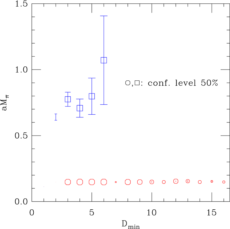
Figure 9: Fit plot showing ground state and excited state masses of Goldstone pion $0^{-+}$ as a function of $D_{\rm min}$, the minimum distance included in the fit. This is from the run with $10/g^{2}=7.09$, $am_{l/s}=0.0062/0.031$, with fits using $D_{\rm max}=28$. The symbol size is proportional to confidence level.

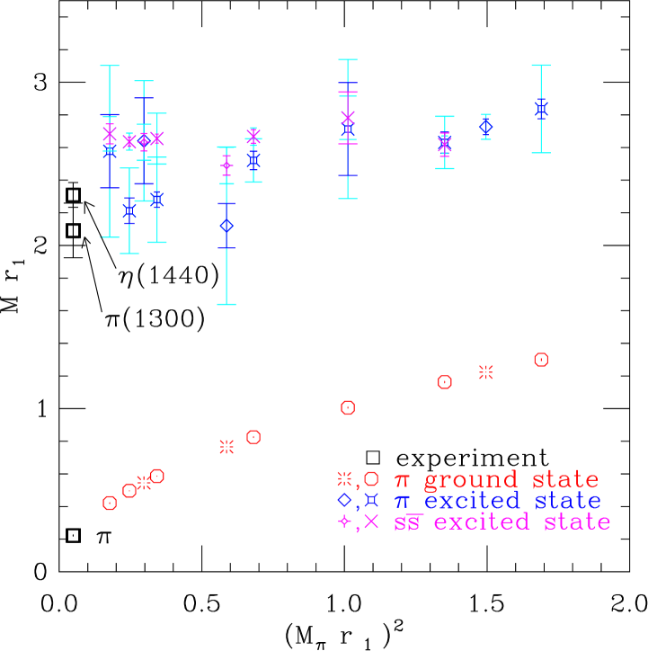
Figure 10: Ground state and excited state $0^{-+}$ masses as a function of $(M_{\pi}r_{1})^{2}$. In the legend, the symbol on the left represents fine lattice results, and that on the right the coarse lattice results.

Figure 10 summarizes the two-state fits for the $0^{-+}$ masses as a function of $(M_{\pi}r_{1})^{2}$. These excited state masses fit a linear function of $(M_{\pi}r_{1})^{2}$ to a 12% confidence level. As the statistical errors on the excited pion mass fits are large compared with the differences between the coarse and fine lattice fits, we considered all of the mass fits together in the linear fit. Extrapolating the resulting linear function to the physical value of $(M_{\pi}r_{1})^{2}=0.050$, we get a prediction of a physical $0^{-+}$ excited state at 1362(41)(247)MeV, which agrees within the large errors with the mass of the $\pi(1300)$ state. The first error is statistical. The second is the systematic error predominantly due to contributions to the propagator which are unaccounted for in the form of the fitting function. We estimate this by examining the fit plots and estimating the range of mass values one might reasonably choose, that is, this error reflects the stability of the fitted value under variation of the fit range, e.g., the difference between the $D_{min}=3$ and $D_{min}=4$ points in Figure 9 and is reflected in Figures 10 and 14 as light cyan error bars on the excited states. We linearly extrapolate the individual systematic errors to $(M_{\pi}r_{1})^{2}=0.05$. Systematic errors due to chiral extrapolation, finite lattice size and lattice spacing, are small relative to the statistical error and the systematic error from additional states.

Similarly, an excited state is evident in the $0^{-+}$ $s\overline{s}$ propagator. The analysis of states containing strange quarks is complicated by the fact that our simulated strange quark masses, $am_{s}=0.050,0.031$ differ from the physical strange quark mass, $am_{s}^{*}=0.039,0.027$ (for the coarse and fine lattices respectively) as discussed in subsection IV.1. To correct for this, after fitting to the form of Eq. (7), we interpolated the meson masses to the correct physical values of the strange quark mass, $m_{s}^{*}$, using

$$M_{\rm PS}(m_{s}^{*})=M_{\rm PS}(m_{s})-(m_{s}-m_{s}^{*})\frac{M_{\rm PS}(m_{s})-M_{\rm PS}(m_{u,d})}{m_{s}-m_{u,d}},$$ (8)

where we use the mass of the excited $0^{-+}$ state at the simulation value of $m_{s}$ for $M_{\rm PS}(m_{s})$, and the pion excited state on the same lattices for $M_{\rm PS}(m_{u,d})$. We cannot interpolate masses from lattices with three flavors of degenerate quarks in this manner, so we eliminate them from this analysis.

The interpolated excited state masses fit a linear function of $(M_{\pi}r_{1})^{2}$ and we again extrapolated the resulting form to the physical $(M_{\pi}r_{1})^{2}$. The result is $M_{s\overline{s}}=1645(40)(145)$ for the excited $s\overline{s}$ psuedoscalar state.

We have no pure $s\overline{s}$ physical $0^{-+}$ with which to compare ground state fits. We can, however, compare the extrapolation of the corrected excited state masses with the experimental mass of the $\eta(1440)$, which one expects to be dominated by the $s\overline{s}$ contribution. This is consistent with our result with the large systematic error. We display all of the pion and (corrected) $0^{-+}$ $s\overline{s}$ fits in Figure 10, with physical states for comparison.

Even more interesting is the kaon propagator. Formed of a light quark and a strange quark, the kaon, $J^{P}=0^{-}$, has no definite charge-conjugation quantum number when $m_{u,d}\neq m_{s}$. Consequently, it has a non-exotic parity partner with $J^{P}=0^{+}$, and the propagator has a tiny, but significant oscillating component. On theses lattices the amplitude of the oscillating state is significantly smaller than that of the kaon ground state, and the mass is greater than that of the kaon ground state, thus it does not interfere with with single-exponential fits of the propagator at large time separations ($D_{\min}>14$). Two-state fits to the form of Eq. (7) fail at all time separations because the $0^{+}$ mass falls below that of the first excited $0^{-}$ state. Figure 11 shows an attempt to fit the $10/g^{2}=7.09$, $am_{u,d}=0.0062$, $am_{s}=0.031$ fine lattice propagator to two non-oscillating exponentials, as in Eq. (7). All fits are of extremely low confidence levels and there is no evident plateau for the excited state. Figure 12 shows fits of the same propagator to a three-state form,

$$C(t)=A_{0}(e^{-M_{0}t}+e^{-M_{0}(T-t)})+A_{1}(e^{-M_{1}t}+e^{-M_{1}(T-t)})+A_{2}(-1)^{t}(e^{-M_{2}t}+e^{-M_{2}(T-t)}),$$ (9)

with high confidence levels and masses of consistent value through a large variation in the lower limit of the fit range, $D_{\rm min}$.

Propagators from both fine lattice sets with $m_{u,d}\neq m_{s}$ were inconsistent with double exponential forms, (Eq. 7), but fit to triple exponentials, (Eq. 9) with high confidence. The same was true of the coarse lattice sets with $am_{u,d}\leq 0.02$. In general, we find that as $m_{u,d}\longrightarrow m_{s}$, the amplitude of the oscillating state becomes indistinguishable from zero, presumably because charge conjugation regains its status as a good quantum number. In the fits to kaon propagators from the coarse lattice set with $10/g^{2}=6.79$, $am_{u,d}=0.030$ we were no longer able to distinguish the amplitude of any oscillating state from noise. Confidence levels for both two-state and three-state fits were a few tenths of a percent, yet we could discern equivalent plateaus for the excited $0^{-}$ state mass as a function of $D_{\rm min}$ in each case. Attempts to read a plateau for the oscillating state were unconvincing. For the coarse lattices with $10/g^{2}=6.81$, $am_{u,d}=0.040$, and both coarse and fine lattices with three degenerate flavors of quarks, two state fits resolved the excited state with high confidence (as we have mentioned before when we considered these very same fits as limiting cases of both pions and $0^{-+}$ $s\overline{s}$ mesons.)

The oscillating scalar state is far lighter than the lightest strange $0^{+}$ meson, the $K_{0}^{*}(1430)$. It does, however, agree well with the sum of the masses of the dominant $K_{0}^{*}(1430)$ decay mode products, $K+\pi$, on every lattice set for which it was measured. Resolution of the $K_{0}^{*}(1430)\rightarrow K+\pi$ decay channel is additional evidence that our simulations with light dynamical quarks correctly reproduce the expected complexities of the physical world. When we perform similar fits to quenched kaon propagators we can find no evidence of an oscillating $0^{+}$ state, even with widely separated valence quark masses, such as $am_{l/s}=0.0062/0.031$. Furthermore, with the quenched kaon propagators, it is simple to extract the contribution of the first excited $0^{-}$ state, see for example Fig. 13.

We have also performed an extrapolation of the excited kaon state masses to the physical value of $(M_{\pi}r_{1})^{2}=0.050$. Again considering the fine and coarse lattice data together the excited states fit, with 8% confidence level, to a line which intercepts $(M_{\pi}r_{1})^{2}=0.050$ at 1527(46)(68)MeV. This is in decent agreement with the K(1460) state and inconsistent with the K(1460)’s expected decay products, $\pi\pi K$, which should be at about 775 MeV. This lends credence to the belief that the K(1460) is a true mesonic state.

Figure 14 summarizes the fits to the kaon propagators. As with the $s\overline{s}$ states, we have corrected the ground state and excited state mass fits for the difference between the simulated strange quark mass and the physical strange quark mass using the interpolation expression (8). Since we have measured a $0^{+}$ state at only one value of the strange quark mass for each lattice spacing, interpolation of the $0^{+}$ state is not possible. We include the pion ground state and the sum of the pion and (uncorrected) kaon ground state masses for comparison. We include isospin-averaged physical states for comparison. We display these results numerically in Table 12.

$10/g^{2}$	$am_{u,d}/am_{s}$	$N_{\rm states}$	$aM_{0^{+}}$	$A_{0^{+}}$	$aM_{\pi}+aM_{K}$	$aM_{K_{\rm ex}}$	range	conf
6.85	0.05	2	—	—	0.97	1.05(2)(10)	3-18	0.36
6.83	0.04/0.05	2	—	—	0.90	1.02(3)(2)	4-32	0.36
6.81	0.03/0.05	2	—	—	0.81	1.07(3)(5)	4-26	0.008
6.79	0.02/0.05	3	0.63(12)(10)	$-3(2)$	0.72	0.96(3)(2)	3-16	0.39
6.76	0.01/0.05	3	0.76(15)(4)	$-13(9)$	0.61	1.00(5)(6)	3-16	0.27
6.76	0.007/0.05	3	0.58(4)(3)	$-10(2)$	0.56	0.97(3)(3)	3-16	0.28
6.76	0.005/0.05	3	0.60(6)(4)	$-24(6)$	0.53	0.98(3)(4)	3-21	0.56
7.18	0.031	2	—	—	0.64	0.71(1)(4)	5-25	0.83
7.11	0.0124/0.031	3	0.47(6)	$-7(3)$	0.48	0.64(2)(3)	5-30	0.49
7.09	0.0062/0.031	3	0.43(2)	$-22(3)$	0.40	0.69(2)(3)	4-30	0.64

Table 12: Results of two- and three-state fits to $0^{-}$ kaon propagators.

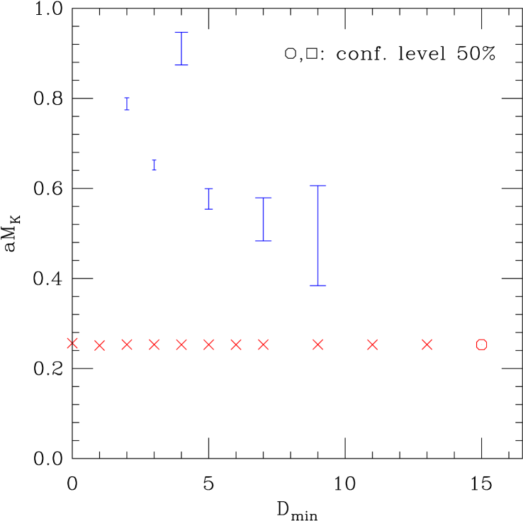
Figure 11: Two-state fits to three-flavor kaon pseudoscalar propagators as a function of minimum distance included in the fit from the run with $10/g^{2}=7.09$ and $am_{l/s}=0.0062/0.031$. The size of the symbols is proportional to the confidence level of the fit. Octagons and squares represent the two $0^{-}$ states, although, as discussed in the text, all of the confidence levels for this fit are so low that these symbols are extremely small. Standard size crosses are used for points where both the error bar and the confidence level are too small to be visible otherwise. These fits used $D_{\rm max}=30$.

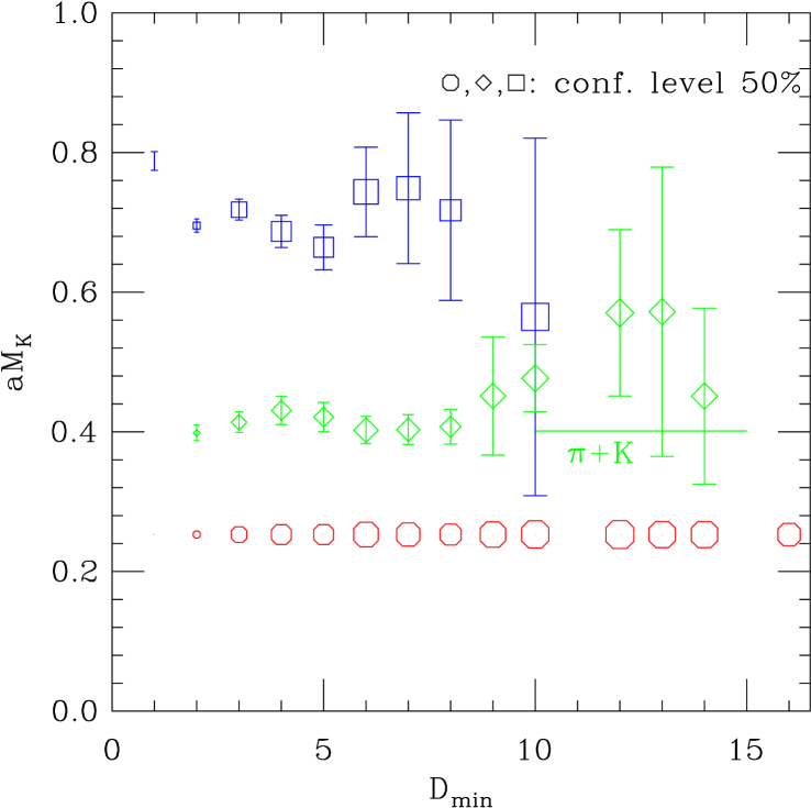
Figure 12: Three-state fits to three-flavor kaon pseudoscalar propagators as a function of minimum distance included in the fit from the run with $10/g^{2}=7.09$ and $am_{l/s}=0.0062/0.031$. The size of the symbols is proportional to the confidence level of the fit. Octagons and squares represent the two $0^{-}$ states; diamonds represent the oscillating $0^{+}$ state. $D_{\rm max}=30$.

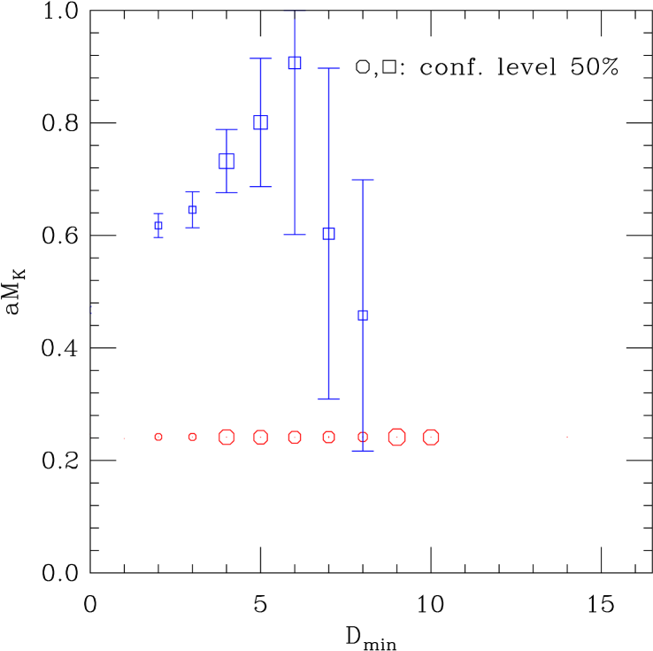
Figure 13: Quenched kaon mass fit plot showing ground state and first excited state, with $10/g=8.40$, $am_{l/s}=0.0062,0.031$, and $D_{\rm max}=17$. Fit to Eq. (7) without an oscillating state.

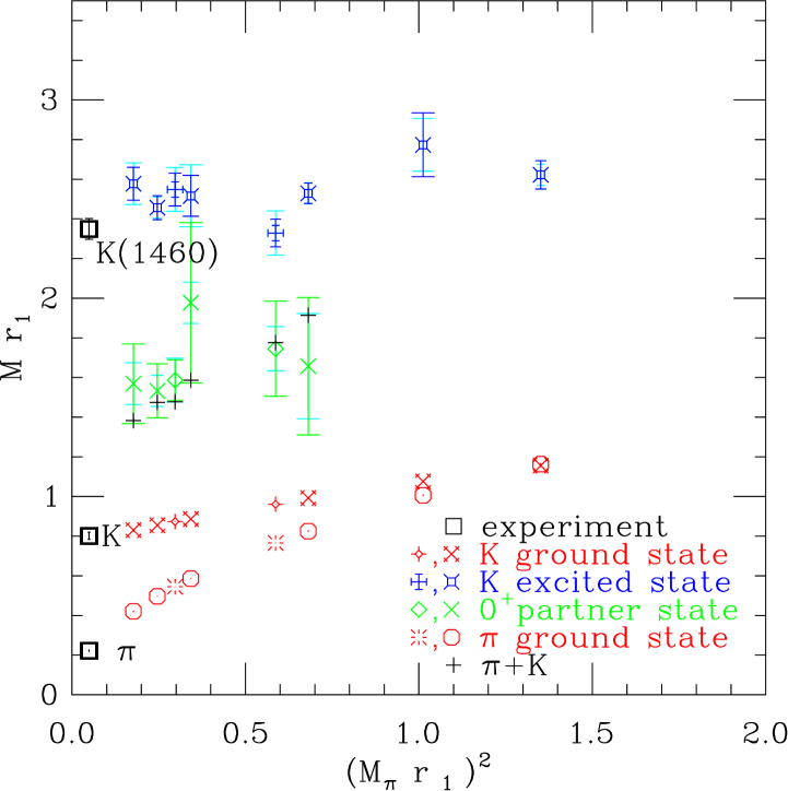
Figure 14: Summary of fits of kaon propagators. Ground state and excited state kaon masses are interpolated to the correct strange quark mass. $0^{+}$ parity partner state and $\pi+K$ masses are uncorrected for comparison. For the $K$s, $\pi$ and $0^{+}$ entries in the legend, the symbol on the left represents fine lattice results, and that on the right the coarse lattice results.

It is worth pointing out that we fit these excited state masses in wall source propagators that were designed specifically to minimize the contribution of excited states. It is likely that analysis with other quark sources would further enhance our ability to resolve excited states.

We note that the consistency of the excited $K$ and $\pi$ states with experiment indicates that there is no unphysical scale in these channels of length $\raise 1.29167pt\hbox{$>$\kern-7.5pt\lower 4.30554pt\hbox{$\sim$}}2$ lattice spacings. This is encouraging, since non-localities that might be introduced by taking the fourth root of the staggered determinant could show up here.

VII Conclusions

In this project we have calculated hadron masses including the effects of three flavors of dynamical quarks, using light quark masses down to $0.1\,m_{s}$ and lattice spacings of about $0.12$ and $0.09$ fm. These quark masses are light enough that we are beginning to “see hadronic decays” in the sense that the lowest energy states for some quantum numbers may be two-meson states instead of a single particle. To the extent that we can reasonably expect, our spectrum results are consistent with the experimental hadron spectrum. One quantity that is sensitive to the effects of sea quarks is “$J$”, which is roughly the derivative of the vector meson mass with respect to the squared pseudoscalar massUKQCD_J . In particular, we plot

$$J=\frac{M_{K^{*}}\left(M_{\phi}-M_{\rho}\right)}{2\left(M_{K}^{2}-M_{\pi}^{2}\right)}\ \ \ .$$ (10)

This quantity is plotted in Fig. 15, which updates results from MILC_spectrum1 , and also includes recent points from the CP-PACS/JLQCD collaborationKaneko2003 .

Comparison of lattice results with the physical spectrum still requires extrapolations to zero lattice spacing and to the physical quark masses. In principle, the extrapolation to zero lattice spacing is straightforward — we expect errors proportional to $a^{2}g^{2}$. Extrapolation to the physical light quark mass is more difficult. First, most of the hadrons decay strongly, and as we have seen for the $0^{++}$, and the $0^{+}$ for nondegenerate quarks, simulations with light sea quark masses show the couplings to the decay channels. For stable hadrons the extrapolation to physical light quark mass involves chiral logarithms. Because of the remaining breaking of taste symmetry, fitting to the chiral logarithms requires that the continuum extrapolation be done first, or simultaneously.

In the case of the pseudoscalar masses and decay constants, taste violations have been included in the chiral perturbation theory, which makes possible a simultaneous extrapolation in lattice spacing and quark massesMILC_fpi ; MILC_fpi_in-prep . The small statistical errors on pseudoscalar masses and decay constants make this rather involved analysis necessary, but also make it possible. Work towards comparable extrapolations for some other quantities, such as the nucleon mass, is in progress.

In the meantime, it is interesting to use a less sophisticated extrapolation to see how these lattice results compare with the real world. Figure 16 shows such a comparison, using a linear or quadratic extrapolation in the light quark mass and linear extrapolation in the squared lattice spacing. Since the difference between the strange quark mass used in our simulations and the correct value is roughly twice as large in the coarse runs as in the fine runs, the extrapolation in lattice spacing also largely corrects for the too-large strange quark mass used in the runs. (It is not entirely an accident that the continuum extrapolation largely takes care of adjusting the strange quark mass, since one of the largest reasons for the error in adjusting the strange quark mass was the neglect of order $a^{2}$ corrections in tuning the strange quark mass.) Note that the lattice nucleon mass plotted here is the linear extrapolation shown in Fig. 4; a proper chiral extrapolation is expected to lower this value.

The spectrum results from these simulations with three dynamical light flavors are encouraging. Clearly, however, considerably more work is needed, in particular on chiral extrapolations, before we can be confident that the calculations can produce accurate and precise results in all the channels that we have examined. Runs are continuing for $m_{u,d}=0.1m_{s}$ on both coarse and fine lattices.

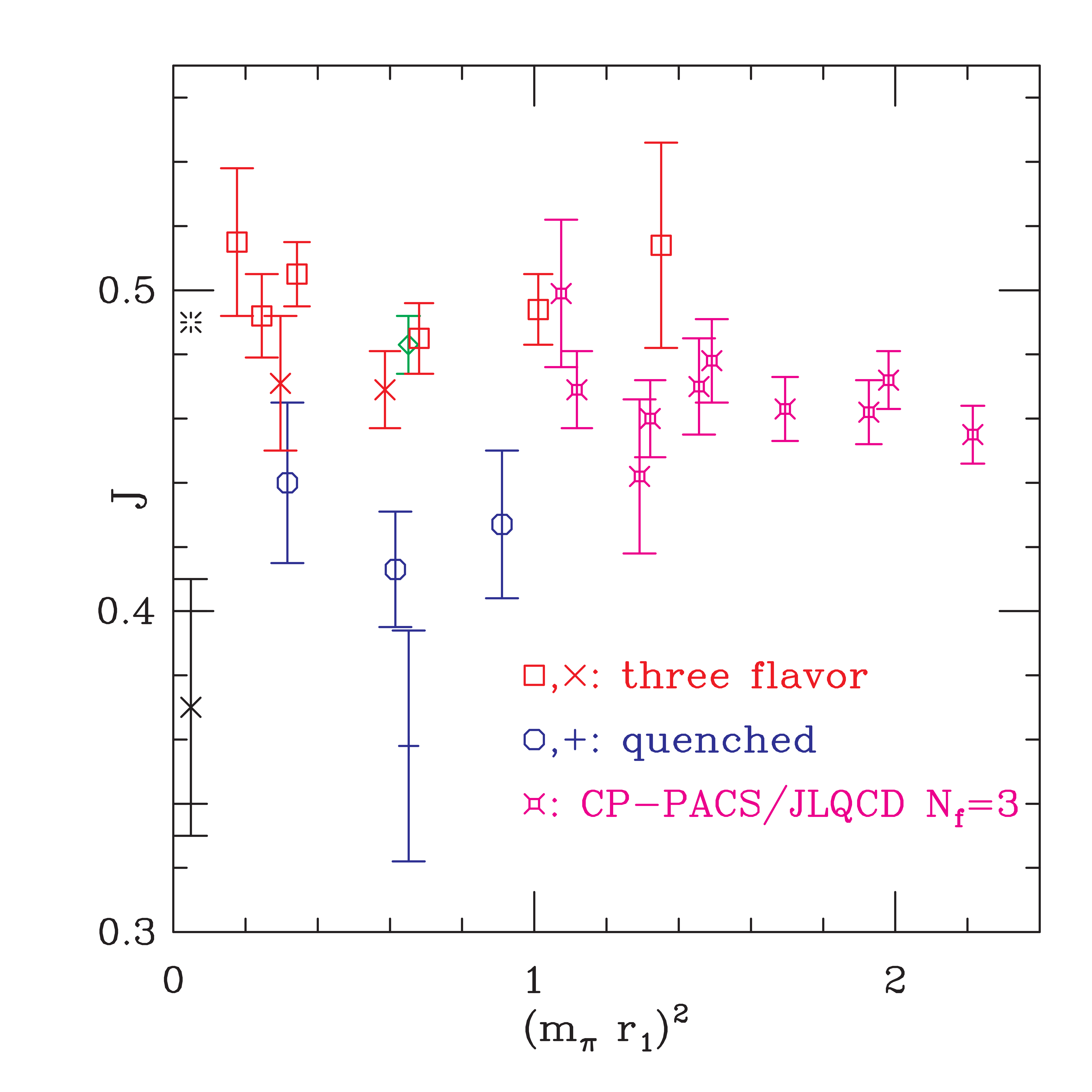
Figure 15: The “J” parameter. The red squares and crosses are three flavor coarse and fine lattice results respectively. The blue octagons and plus signs are quenched coarse and fine results, while the green diamond is a two flavor run. The magenta decorated squares are CP-PACS/JLQCD three flavor Wilson quark resultsKaneko2003 . The cross at the left is the original UKQCD quenched estimateUKQCD_J , and the burst at the left is the experimental value.

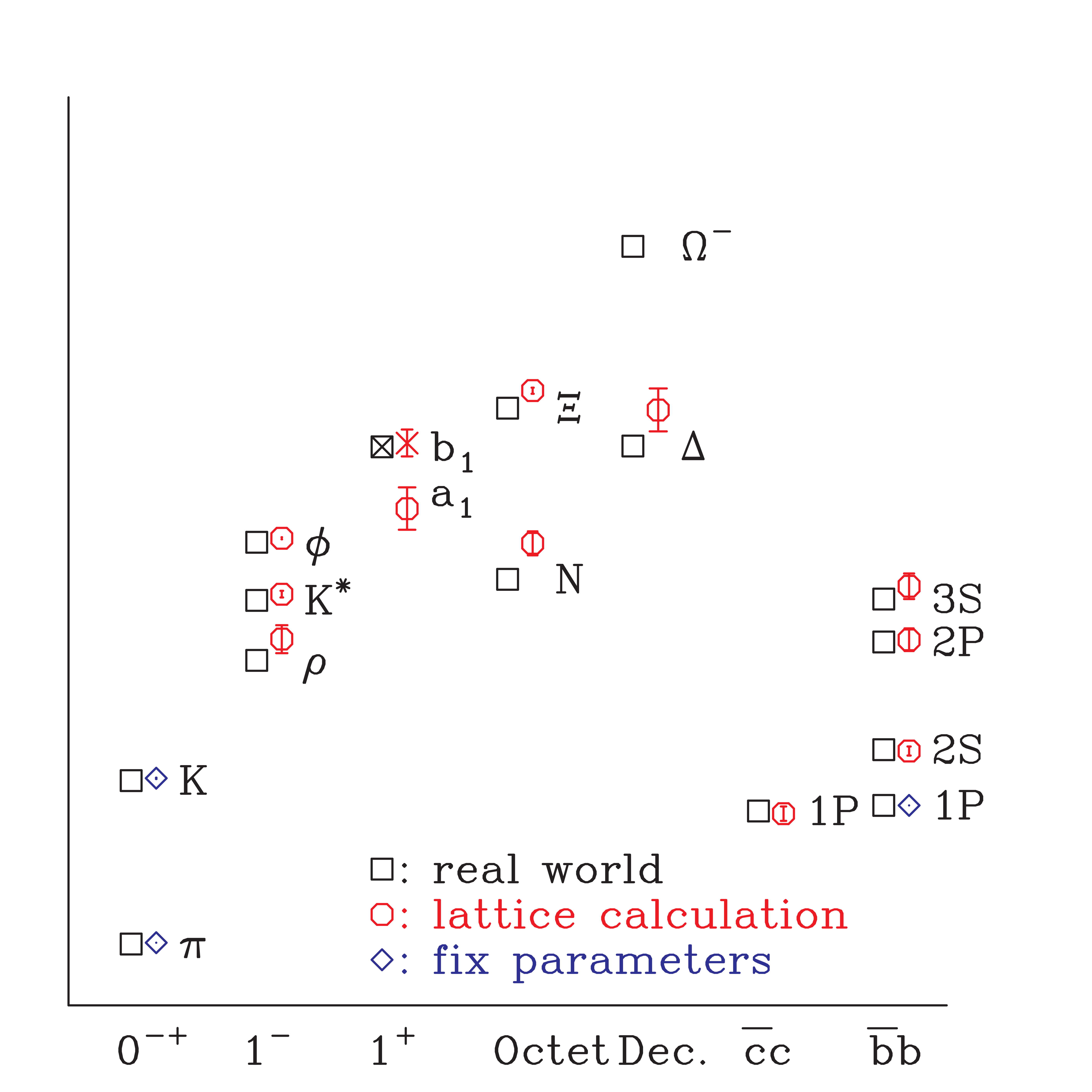
Figure 16: The “big picture”. Crude continuum and chiral extrapolations of hadron masses and splittings compared with experimental values. The upsilon and charmonium columns are differences from the ground state masses, from work of the HPQCD and Fermilab groupsHPQCD_private ; PRL . Here the $\pi$ and $K$ masses fix the light and strange quark masses, and the $\Upsilon$ 1P-1S mass splitting is used to fix the lattice spacing.

References

- (1) The MILC Collaboration, C. Bernard et al., Phys. Rev. D 64 (2001) 054506;
- (2) Some preliminary results may be found in The MILC Collaboration, C. Bernard et al., Nucl. Phys. Proc. Suppl. 119, 257 (2003).
- (3) The MILC Collaboration, C. Bernard et al., Phys. Rev. D 62, 034503, 2000; The MILC Collaboration, C. Bernard et al., Nucl. Phys. Proc. Suppl. 119, 598 (2003).
- (4) A. Gray et al. [HPQCD collaboration], Nucl. Phys. Proc. Suppl. 119, 592 (2003); M. Wingate, J. Shigemitsu, G. P. Lepage, C. Davies and H. Trottier, Nucl. Phys. Proc. Suppl. 119, 604 (2003).
- (5) M. di Pierro et al., hep-lat/0310045, hep-lat/0310042.
- (6) The MILC Collaboration, C. Bernard et al., Nucl. Phys. (Proc.Suppl.) 106, 412 (2002), 119, 613 (2003); M. Wingate et al., hep-lat/0309092, to be published in Nucl. Phys. B (Proc. Suppl.).
- (7) The MILC Collaboration, C. Aubin et al. hep-lat/0309088, to be published in Nucl. Phys. B (Proc. Suppl.).
- (8) The MILC Collaboration, C. Aubin et al., in preparation.
- (9) C. Davies et al., Nucl. Phys. B (Proc. Suppl.) 119 (2003) 595.
- (10) The MILC Collaboration, C. Bernard et al., Nucl. Phys. Proc. Suppl. 119, 260 (2003); Phys. Rev. D 68, 074505 (2003).
- (11) The MILC Collaboration, C. Bernard et al., Nucl. Phys. Proc. Suppl. 119, 991 (2003); Phys. Rev. D 68, 114501 (2003).
- (12) J. Shigemitsu et al., hep-lat/0309039, to be published in Nucl. Phys. B (Proc. Suppl.); The MILC Collaboration, C. Bernard et al., hep-lat/0309055, to be published in Nucl. Phys. B (Proc. Suppl.); M. Okamoto et al., hep-lat/0309107.
- (13) J. Hein, C. Davies, G. P. Lepage, Q. Mason and H. Trottier [HPQCD Collaboration], Nucl. Phys. Proc. Suppl. 119, 317 (2003).
- (14) The HPQCD, MILC, and UKQCD Collaborations, C. Aubin et al., in preparation.
- (15) W. Schroers et al. hep-lat/0309065, to be published in Nucl. Phys. B (Proc. Suppl).
- (16) C.T.H. Davies et al., Phys. Rev. Lett. 92 (2004) 022001; S. Gottlieb, hep-lat/0310041.
- (17) S. Gottlieb et al., Phys. Rev. D 35, 2531 (1987).
- (18) UKQCD Collaboration, S.P. Booth et al., Phys. Lett. B294, 385 (1992).
- (19) C. Davies and G.P. Lepage, HPQCD collaboration, private communication; M. Wingate, et al., hep-ph/0311130.
- (20) G.P. Lepage and P. Mackenzie, Phys. Rev. D 48, (1993) 2250.
- (21) W. Lee and S. Sharpe, Phys. Rev. D 60 (1999) 114503.
- (22) C. Aubin and C. Bernard, Phys. Rev. D 68, (2003) 034014 (2003) [hep-lat/0304014] and Phys. Rev. D 68, (2003) 074011 [hep-lat/0306026]; The MILC Collaboration, C. Aubin et al., hep-lat/0309088.
- (23) E. Jenkins, Nucl. Phys. B368, 190 (1992); D.B. Leinweber, A.W. Thomas, K. Tsushima, S.V. Wright, Phys. Rev. D 61 (2000) 074502; Nucl. Phys. B (Proc.Suppl.) 83 (2000) 179.
- (24) V. Bernard, N. Kaiser and U.G. Meissner. Z. Phys C60, 111 (1993).
- (25) W. A. Bardeen, A. Duncan, E. Eichten, N. Isgur and H. Thacker, Phys. Rev. D 65, (2002) 014509.
- (26) The MILC Collaboration, C. Bernard et al., hep-lat/0309117, to appear in Nucl. Phys. B (Proc. Suppl.).
- (27) CP-PACS/JLQCD collaboration: T. Kaneko et al., hep-lat/0309137, to appear in Nucl. Phys. B (Proc. Suppl.).
- (28) P. Lacock and C. Michael, Phys. Rev. D 52, 5213 (1995).