Numerical Portrait of a Relativistic BCS Gapped Superfluid Numerical Portrait of a Relativistic BCS Gapped Superfluid Numerical Portrait of a Relativistic BCS Gapped Superfluid

Abstract

We present results of numerical simulations of the 3+1 dimensional Nambu – Jona-Lasinio (NJL) model with a non-zero baryon density enforced via the introduction of a chemical potential $\mu\neq 0$. The triviality of the model with a number of dimensions $d\geq 4$ is dealt with by fitting low energy constants, calculated analytically in the large number of colors (Hartree) limit, to phenomenological values. Non-perturbative measurements of local order parameters for superfluidity and their related susceptibilities show that, in contrast with the 2+1 dimensional model, the ground-state at high chemical potential and low temperature is that of a traditional BCS superfluid. This conclusion is supported by the direct observation of a gap in the dispersion relation for $0.5\leq\mu a\leq 0.85$, which at $\mu a=0.8$ is found to be roughly $15\%$ the size of the vacuum fermion mass. We also present results of an initial investigation of the stability of the BCS phase against thermal fluctuations. Finally, we discuss the effect of splitting the Fermi surfaces of the pairing partners by the introduction of a non-zero isospin chemical potential.

I Introduction

The ground state of QCD with $N_{f}\geq 3$ flavors of light quark at low temperature $T$ and asymptotically high density is thought to be a “color-flavor locked” (CFL) state in which SU(3)${}_{c}\otimes$SU$(N_{f})_{L}\otimes$SU$(N_{f})_{R}\otimes$U(1)_B symmetry is spontaneously broken by diquark condensation in the color anti-triplet channel to a diagonal SU(3)_Δ, and which is thus simultaneously color superconducting, superfluid, and chirally broken Alford et al. (1999); Schafer and Wilczek (1999). Since diquark condensation is thought to occur at the Fermi surface via a BCS mechanism, it is accurately described by a self-consistent gap equation in the asymptotic regime $\mu\to\infty$, with $\mu$ the quark chemical potential or Fermi energy, where the QCD coupling $g(\mu)$ is weak Rischke (2004). However, the densities for which analytic predictions of weakly-coupled QCD can be trusted are much greater than the conditions, with $\mu\sim O(1{\rm GeV})$, which are likely to be physically realisable in our universe at the centres of compact stars Alford et al. (2001a).

In this regime we face the twin problems that QCD becomes strongly interacting, and that the most systematic way of computing its properties non-perturbatively, namely numerical simulation of lattice gauge theory, cannot help because of the “sign problem”; the lack of positivity of the QCD Euclidean path integral measure with $\mu\not=0$ makes Monte Carlo sampling methods inoperable. Another complicating factor is that once the density becomes low enough to make the strange quark mass $m_{s}$ no longer negligible compared to $\mu$, then other channels involving pairing between just $u$ and $d$ may be preferred, leading to a plethora of different possible ground states, including even crystalline examples Rajagopal and Wilczek (2001); Alford (2001); Bowers and Rajagopal (2002). Analytic approaches to these questions must either use some approximate non-perturbative approach such as the instanton liquid Rapp et al. (1998), or resort to phenomenological models of the strong interaction such as the Nambu – Jona-Lasinio (NJL) model Alford et al. (1998); Berges and Rajagopal (1999).

Generic NJL models contain fermions, to be thought of either as quarks or baryons, self-interacting via contact four-Fermi terms Nambu and Jona-Lasinio (1961). In a Euclidean metric, the prototype is written in terms of isopinor fermion fields $\psi,\bar{\psi}$, as

$${\cal L}_{NJL}=\bar{\psi}(\partial{\!\!\!/\,}+m)\psi-\frac{g^{2}}{2}\left[(\bar{\psi}\psi)^{2}-(\bar{\psi}\vec{\tau}\gamma_{5}\psi)^{2}\right],$$ (1)

which has SU(2)${}_{L}\otimes$SU(2)_R chiral symmetry. In 3+1 dimensions the interaction strength $g^{2}$ has mass dimension -2, implying that the model is non-renormalisable and must be defined in terms of some explicit ultra-violet scale $\Lambda$ (see e.g. Hands and Kogut (1998)). Since the model has no gluons, it fails to reproduce the physics of confinement; however, for sufficiently large $g^{2}$ the model does exhibit spontaneous chiral symmetry breaking to SU(2)_I, resulting in a physical or “constituent” fermion mass scale $\Sigma\sim g^{2}\Lambda^{3}\gg m$. The phase structure of the model is most conveniently studied in the Hartree approximation, corresponding to retaining only those diagrams which, if the number of fermion degrees of freedom were multiplied by a factor $N$ and the coupling rescaled as $g^{2}/N$, would remain at leading order in $1/N$. At low $T$ it is found that for values of chemical potential $\mu_{c}\sim\Sigma$ there is a transition, whose order depends on the details of the cutoff, in which chiral symmetry is restored and baryon density $n_{B}=\langle\bar{\psi}\gamma_{0}\psi\rangle$ increases sharply from zero  Hatsuda and Kunihiro (1985); Asakawa and Yazaki (1989); Klevansky (1992). For $\mu>\mu_{c}$ the NJL model thus describes a state resembling relativistic “quark matter.” Since there is no short-range repulsion present, the stability of a phase in which both $n_{B}$ and $\Sigma$ are simultaneously non-zero, corresponding to “nuclear matter,” is not a priori clear.

The color superconducting solutions discussed in the first paragraphs have been obtained by solving the self-consistent “gap equation” for the smallest energy $2\Delta$ required to excite a quasiparticle pair out of the ground state consisting of a filled Fermi sea. Solutions with $\Delta>0$, implying the instability of a sharp Fermi surface with respect to formation of a condensate of Cooper pairs, form the basis of the BCS description of superconductivity Bardeen et al. (1957). Such solutions are also characterised by a Cooper pair or diquark condensate $\langle qq\rangle\not=0$ whose precise definition will be given below; here it suffices to identify it with the density of condensed pairs in the ground state. Since the NJL model is not a gauge theory the corresponding BCS ground state is not superconducting (analogous to a Higgs vacuum in particle physics), but rather a superfluid, in which the global U(1)_B baryon number symmetry of (1) is spontaneously broken by $\langle qq\rangle\not=0$, which is thus a true order parameter.

Since to leading order in $1/N$ $\langle qq\rangle=\Delta=0$, it is legitimate to query the approximate methods used to find such solutions. Fortunately in this case it is possible to employ numerical lattice methods, because as reviewed below the lattice-regularised NJL model has no sign problem. Initial studies have focused on the high density phase of the NJL model in 2+1$d$, in part for the obvious technical advantage of working in reduced dimensionality, and in part for the conceptual advantage that NJL₂₊₁ has an ultra-violet stable fixed point and hence an interacting continuum limit, so that in principle we need not worry about the cutoff dependence of the results. Although the simulations reveal enhanced diquark pairing in the scalar isoscalar channel Hands and Morrison (1999), there is no evidence for the expected BCS signal $\langle qq\rangle\not=0$, $\Delta\not=0$. Instead, the condensate vanishes non-analytically with external diquark source strength $j$, and the fermion dispersion relation reveals a sharp Fermi surface and massless quasiparticles Hands et al. (2001a, 2002). The fitted values for the Fermi momentum and Fermi velocity, however, do not match those of free field theory, and indeed are difficult to account for in orthodox Fermi liquid theory Hands et al. (2003). The interpretation is that due to its low dimensionality the system realises superfluidity in an unconventional Berezinskii-Kosterlitz-Thouless (BKT) mode first invoked to describe thin helium films Nelson (1983); the massless modes due to phase fluctuations of the would-be condensate field remain strongly fluctuating, resulting in unbroken U(1)_B symmetry but critical behaviour for all $\mu>\mu_{c}$. Metastability of persistent flow is only revealed by the non-trivial response of the system to a symmetry breaking field with a twist imposed across the spatial boundary.

For this reason in the current paper we present results of simulating NJL₃₊₁, with the goal of exposing superfluid behaviour with the more conventional signal $\langle qq\rangle\not=0$, $\Delta>0$. Our first results suggesting that $\langle qq\rangle\not=0$ for $\mu>\mu_{c}$ have appeared in Hands and Walters (2002). The details of the lattice model, the simulation technique, and the observables monitored to expose this behaviour are reviewed below in Sec. II. As already stated, in 3+1$d$ the model is non-renormalisable and must be defined with a cutoff. The bare parameters $g^{2}$ and $m$ must be chosen so that the model’s properties match those of low energy QCD as closely as possible; in Sec. II.3 we use a large-$N$ expansion (here $N$ is identified with the number of “colors” $N_{c}$) to calculate the vacuum fermion mass $\Sigma_{0}$ and the constants $f_{\pi}$ and $m_{\pi}$, and find that a reasonable matching can be made with an inverse lattice spacing $a^{-1}\simeq 700$MeV. In Sec. III we present results for the phase structure of the model for low $T$, the diquark condensate and associated susceptibilities, and in Sec. IV dispersion relations in the spin-$\frac{1}{2}$ sector. For the first time there is evidence for a non-vanishing BCS gap from a lattice simulation, with $\Delta/\Sigma_{0}\simeq 0.15$, which translates to a gap of around 60MeV in physical units. This is consistent with estimates from self-consistent approaches Berges and Rajagopal (1999); Nardulli (2002). In Sec. V we discuss finite volume effects and finally in Secs. VI and VII present preliminary results for simulations both with $T>0$ and with small but non-zero isospin chemical potential $\mu_{I}\not=0$, which has the effect of separating the $u$ and $d$ quark Fermi surfaces and hence discouraging $ud$ condensation. Sec. VIII contains a brief summary.

II Lattice Model and Parameter Choice

II.1 Formulation and symmetries

The lattice version of the NJL model we employ was first used in a study of chiral symmetry restoration at zero chemical potential in Hands and Kogut (1998). The action, with lattice spacing $a$ set to unity, reads

$$S_{0}=S_{ferm}+S_{bos}=\sum_{xy}\bar{\chi}_{x}M[\Phi]_{xy}\chi_{y}+\bar{\zeta}_{x}M^{*}[\Phi]_{xy}\zeta_{y}+\frac{2}{g^{2}}\sum_{\tilde{x}}\mbox{tr}\Phi^{\dagger}_{\tilde{x}}\Phi_{\tilde{x}},$$ (2)

where $\chi,\bar{\chi},\zeta$ and $\bar{\zeta}$ are Grassmann-valued staggered isospinor fermion fields defined on the sites $x$ of a hypercubic lattice, and $\Phi\equiv\sigma+i\vec{\pi}.\vec{\tau}$ is a $2\times 2$ matrix of bosonic auxiliary fields defined on the dual sites $\tilde{x}$. The kinetic operator $M$ is given by

$$M_{xy}^{pq} = {\frac{1}{2}}\delta^{pq}\left[e^{\mu}\delta_{yx+\hat{0}}-e^{-\mu}\delta_{yx-\hat{0}}+\sum_{\nu=1,2,3}\eta_{\nu}(x)(\delta_{yx+\hat{\nu}}-\delta_{yx-\hat{\nu}})+2m\delta_{xy}\right]$$ (3)

$$+ {\frac{1}{16}}\delta_{xy}\sum_{\langle\tilde{x},x\rangle}\left(\sigma(\tilde{x})\delta^{pq}+i\varepsilon(x)\vec{\pi}(\tilde{x}).\vec{\tau}^{pq}\right)$$

such that the parameters are bare fermion mass $m$, coupling $g^{2}$ (with mass dimension -2) and baryon chemical potential $\mu$. The symbol $\langle\tilde{x},x\rangle$ denotes the set of 16 dual sites adjacent to $x$. The Pauli matrices acting on isospin indices $p,q$ are normalised so that $\mbox{tr}\tau_{i}\tau_{j}=2\delta_{ij}$. The phase factors $\eta_{\nu}(x)=(-1)^{x_{0}+\cdots+x_{\nu-1}}$ and $\varepsilon(x)=(-1)^{x_{0}+x_{1}+x_{2}+x_{3}}$ ensure that fermions with the correct Lorentz covariance properties emerge in the continuum limit, and that in the limit $m\to 0$ the action (2) has a global SU(2)${}_{L}\otimes$SU(2)_R invariance under

$$\chi\mapsto({\cal P}_{e}U+{\cal P}_{o}V)\chi\;\; \;\;\bar{\chi}\mapsto\bar{\chi}({\cal P}_{e}V^{\dagger}+{\cal P}_{o}U^{\dagger})$$ ;

$$\zeta\mapsto({\cal P}_{e}U^{*}+{\cal P}_{o}V^{*})\zeta\;\; \;\;\bar{\zeta}\mapsto\bar{\zeta}({\cal P}_{e}V^{\dagger*}+{\cal P}_{o}U^{\dagger*})$$ ;

$$\Phi \mapsto V\Phi U^{\dagger}\;\;\;\;\mbox{with}\;\;\;U,V\in\mbox{SU(2)}.$$ (4)

The even/odd projectors are given by ${\cal P}_{e/o}(x)={\frac{1}{2}}(1\pm\varepsilon(x))$. In addition the action has a U(1)_B invariance under baryon number rotations:

$$\chi,\zeta\mapsto e^{i\alpha}\chi,\zeta\;\;\;\;\;\bar{\chi},\bar{\zeta}\mapsto\bar{\chi},\bar{\zeta}e^{-i\alpha}.$$ (5)

The auxiliary fields $\sigma$ and $\vec{\pi}$ can be integrated out to yield an action written solely in terms of fermion fields $\chi$ and $\zeta$. In the continuum limit $a\partial\to 0$ lattice fermion doubling leads to a physical content for the model of eight fermion species (four described by $\chi$, four by $\zeta$) with self-interactions resembling those of the continuum NJL model (but with terms of the form $\bar{\chi}\chi\bar{\zeta}\zeta$ differing in detail from those of the form $\bar{\chi}\chi\bar{\chi}\chi$), resulting in an additional approximate U(4)$\otimes$U(4) symmetry which is violated by terms of $O(a)$. Further details are given in Hands and Kogut (1998). In what follows we will somewhat arbitrarily refer to these degrees of freedom as colors and hence define $N_{c}=8$; this is in distinction to the explicit flavor or isospin symmetry (4) which gives rise to $N_{f}=2$.

In order to examine issues associated with diquark pairing, it is necessary to introduce a source term into the action. A suitable term, invariant under (4) but violating baryon number conservation (5), is:

$$S_{source}=\sum_{x}{\frac{j}{2}}(\chi^{tr}_{x}\tau_{2}\chi_{x}+\zeta^{tr}_{x}\tau_{2}\zeta_{x})+{\frac{\bar{\jmath}}{2}}(\bar{\chi}_{x}\tau_{2}\bar{\chi}^{tr}_{x}+\bar{\zeta}_{x}\tau_{2}\bar{\zeta}^{tr}_{x}),$$ (6)

where in this paper we will consider $j,\bar{\jmath}$ real and positive. With this addition the partition function follows from integrating over the Grassmann degrees of freedom:

$$Z[j,\bar{\jmath}] = \int D\chi D\bar{\chi}D\zeta D\bar{\zeta}D\Phi\exp-(S_{ferm}+S_{bos}+S_{source})$$ (7)

$$= \int D\Phi\;\mbox{Pf}^{N_{c}/4}({\cal A}[\Phi,j,\bar{\jmath}])e^{-S_{bos}[\Phi]}$$

with the antisymmetric matrix ${\cal A}(j,\bar{\jmath})$, which acts on bispinors $(\bar{\chi},\chi^{tr})$ (and ${\cal A}^{*}(-j,-\bar{\jmath})$ on $(\bar{\zeta},\zeta^{tr})$), given by

$${\cal A}=\left(\begin{matrix}\bar{\jmath}\tau_{2}&M\cr-M^{tr}&j\tau_{2}\cr\end{matrix}\right).$$ (8)

The reality of $\mbox{Pf}{\cal A}=\sqrt{\mbox{det}{\cal A}}$ follows by noting the identity $\tau_{2}M\tau_{2}=M^{*}$ Hands et al. (2002). In fact, $\mbox{Pf}{\cal A}$ can also be shown to be positive definite Hands et al. (2002, 2000), implying that $Z$ can also be defined for a single power of the pfaffian, (i.e. with the fields $\zeta,\bar{\zeta}$ omitted), corresponding to $N_{c}=4$. However, the smallest value of $N_{c}$ permitted by the exact hybrid Monte Carlo algorithm (see Sec. II.4) is 8.

II.2 Observables

Here we list the various observables monitored in the simulations. For simplicity we restrict our attention to those constructed from the $\chi,\bar{\chi}$ fields; their equivalents in the $\zeta$ sector are easily found. Angled brackets denote averages taken with respect to the measure defined by (7).

The chiral condensate $\langle\bar{\chi}\chi\rangle$ is given by

$$\langle\bar{\chi}\chi\rangle={\frac{1}{V}}{\frac{\partial\ln Z}{\partial m}}={\frac{1}{2V}}\left\langle\mbox{tr}\biggl{(}\begin{matrix}&\openone\cr-\openone&\cr\end{matrix}\biggr{)}{\cal A}^{-1}\right\rangle.$$ (9)

To leading order in a large-$N_{c}$ expansion the chiral condensate is proportional to the expectation value of the scalar field $\Sigma\equiv\langle\sigma\rangle=\frac{g^{2}}{2}\langle\bar{\chi}\chi\rangle$, which in the chiral limit also defines the physical or constituent fermion mass. The baryon charge density $n_{B}$ per flavor is given by

$$n_{B}=\frac{1}{2V}{\frac{\partial\ln Z}{\partial\mu}}={\frac{1}{8V}}\left\langle\mbox{tr}\biggl{(}\begin{matrix}&e^{\mu}\delta_{yx+\hat{0}}+e^{-\mu}\delta_{yx-\hat{0}}\cr-e^{\mu}\delta_{yx-\hat{0}}-e^{-\mu}\delta_{yx+\hat{0}}&\cr\end{matrix}\biggr{)}{\cal A}^{-1}\right\rangle.$$ (10)

In the diquark sector it is convenient to define operators

$$qq_{\pm}(x)={\frac{1}{4}}[\chi^{tr}_{x}\tau_{2}\chi_{x}\pm\bar{\chi}_{x}\tau_{2}\bar{\chi}^{tr}_{x}]$$ (11)

and corresponding source strengths $j_{\pm}=j\pm\bar{\jmath}$. The condensates are then

$$\langle qq_{\pm}\rangle={\frac{1}{V}}{\frac{\partial\ln Z}{\partial j_{\pm}}}={\frac{1}{4V}}\left\langle\mbox{tr}\biggl{(}\begin{matrix}\pm\tau_{2}&\cr&\tau_{2}\end{matrix}\biggr{)}{\cal A}^{-1}\right\rangle.$$ (12)

In the continuum limit, the corresponding operators written in terms of spinors $\psi,\bar{\psi}$ with 4 spin, 2 flavor and 4 color components are Hands et al. (2000)

$$qq_{\pm}\propto\psi^{tr}C\gamma_{5}\otimes\tau_{2}\otimes(C\gamma_{5})^{*}\psi\pm\bar{\psi}C\gamma_{5}\otimes\tau_{2}\otimes(C\gamma_{5})^{*}\bar{\psi}^{tr},$$ (13)

with $C$ the charge conjugation matrix satisfying $C\gamma_{\mu}C^{-1}=-\gamma_{\mu}^{*}$. The condensate wavefunction is thus scalar isoscalar, but with a non-trivial (and for us uninteresting) variation under “color” rotations, and manifestly antisymmetric as required by the exclusion principle. We will also consider the diquark susceptibilities

$$\chi_{\pm}\equiv{\frac{\partial\langle qq_{\pm}\rangle}{\partial j_{\pm}}}=\sum_{x}\langle qq_{\pm}(0)qq_{\pm}(x)\rangle$$ (14)

which are constrained by identities analogous to the axial Ward identity for the pion propagator; a particularly useful form in the $j_{-}\to 0$ limit reads

$$\chi_{-}|_{j_{-}=0}={\frac{\langle qq_{+}\rangle}{j_{+}}}.$$ (15)

When U(1)_B is spontaneously broken by the formation of a condensate $\langle qq_{+}\rangle\not=0$, therefore, $qq_{-}$ interpolates the resulting Goldstone mode, whose masslessness as $j_{+}\to 0$ is guaranteed by (15). Physically the Goldstone mode is responsible for long-range interactions between vortices in the superfluid phase, and at non-zero $T$ for propagating wave excitations of local energy density known as second sound.

In order to study the spectrum in the spin$-{\frac{1}{2}}$ sector we need the Gor’kov propagator ${\cal G}={\cal A}^{-1}$. It can be written as

$${\cal G}_{xy}=\left(\begin{matrix}A_{xy}&N_{xy}\cr\bar{N}_{xy}&\bar{A}_{xy}\cr\end{matrix}\right)$$ (16)

where each entry is a $2\times 2$ matrix in isospace. The notation indicates both normal $\langle q(x)\bar{q}(y)\rangle$ and anomalous $\langle q(x)q(y)\rangle$ components: on a finite system $A$ and $\bar{A}$ vanish in the limit $j,\bar{\jmath}\to 0$, and we recover the usual fermion and anti-fermion propagators as $N$ and $\bar{N}$ respectively. The number of independent components is constrained by the identities $N_{22}\equiv N_{11}^{*}$, $N_{21}\equiv-N_{12}^{*}$, $A_{22}\equiv-A_{11}^{*}$ and $A_{21}\equiv A_{12}^{*}$, so that ${\cal G}$ can be reconstructed using just two conjugate gradient inversions of ${\cal A}$. In addition, isospin and time-reversal symmetries dictate that after averaging over configurations the only independent non-vanishing components are $\mbox{Re}\overline{N}_{11}$ and ${\rm Im}A_{12}$, which henceforth we will refer to simply as $N$ and $A$ respectively.

II.3 Phenomenological Parameter Choice

As previously discussed, in a number of dimensions $d\geq 4$, the continuum NJL model is non-renormalisable, which implies that the lattice model becomes trivial in the continuum limit Klevansky (1992); Hands and Kogut (1998). This means one must choose a fixed lattice spacing $a$, corresponding to a fixed inverse coupling constant $\beta=\frac{a^{2}}{g^{2}}$, by fitting the model’s parameters to low energy, vacuum phenomenology. Employing methods outlined in Klevansky (1992), we calculate the ratio between the pion decay rate $f_{\pi}$ and the constituent quark mass, i.e. the dynamical mass of the quark in the chirally broken phase. By fitting to phenomenological values we may extract $\beta$ as a function of the model’s only other free parameter, the current quark mass $m$. Finally, calculating and fitting the pion mass $m_{\pi}$ allows us to fix $m$, and hence $\beta$. We take advantage of the fact that a perturbative expansion in $1/N_{c}$ is possible in four-Fermi theories by calculating quantities analytically to leading order in $1/N_{c}$, the Hartree approximation. Feynman diagrams are evaluated using staggered quark propagators defined on an $L_{s}^{3}\times L_{t}/2^{4}$ Euclidean blocked lattice with periodic boundary conditions in spatial dimensions and anti-periodic boundary conditions in the temporal dimension. The integrals over loop momenta are evaluated as sums over momentum modes.

Let us first calculate the gap equation, the fermion self-interaction, to leading order in $1/N_{c}$. For sufficiently strong coupling $g^{2}>g_{c}^{2}$ the scalar auxiliary field $\sigma$ develops a spontaneous vacuum expectation value $\Sigma$, which in the chiral limit can be identified with the constituent fermion mass and is given by

$$\begin{array}[]{c c c c c}\Sigma&=&\begin{picture}(30.0,20.0)(0.0,0.0) \put(0.0,0.0){} \put(0.0,0.0){} \put(0.0,0.0){} \end{picture}&=&{\displaystyle\frac{N_{c}N_{f}\Sigma^{*}}{\beta}\int^{\frac{\pi}{2}}_{-\frac{\pi}{2}}\frac{{\rm d}^{4}p}{\left(2\pi\right)^{4}}\frac{1}{\tilde{p}^{2}+\left(\Sigma^{*}a\right)^{2}}},\end{array}$$ (17)

where $\tilde{p}^{2}=\sum_{\nu=0}^{3}\sin^{2}p_{\nu}$ is the dimensionless squared loop momentum, $N_{c}$ and $N_{f}$ are the number of flavors and colors respectively, and $\beta=a^{2}/g^{2}$ is the dimensionless inverse coupling constant. In this section we shall distinguish the expectation value of the scalar field $\Sigma$ from the constituent mass, which to leading order in $(1/N_{c})$ we define as $\Sigma^{*}\equiv\Sigma+m$; elsewhere in this paper the two shall be used interchangeably and both denoted by $\Sigma$.

$f_{\pi}$ is calculated from the vacuum to one-pion axial-vector matrix element

$$\begin{picture}(300.0,30.0)(-140.0,30.0) \put(0.0,0.0){} \put(0.0,0.0){} \put(0.0,0.0){} \put(0.0,0.0){} \put(0.0,0.0){} \raise 35.0pt\hbox to0.0pt{\kern 110.0pt\makebox(0.0,0.0)[b]{$ka^{-1}$}\hss} \ignorespaces \raise 57.5pt\hbox to0.0pt{\kern 43.0pt\makebox(0.0,0.0)[b]{$(p+k/2)a^{-1}$}\hss} \ignorespaces \raise 2.5pt\hbox to0.0pt{\kern 43.0pt\makebox(0.0,0.0)[t]{$(p-k/2)a^{-1}$}\hss} \ignorespaces \raise 30.0pt\hbox to0.0pt{\kern-5.0pt\makebox(0.0,0.0)[r]{$\left<0\left|J_{i5\mu}(k)\right|\pi_{j}\right>=i\gamma_{\mu}\gamma_{5}\frac{\tau_{j}}{2}$}\hss} \ignorespaces \raise 30.0pt\hbox to0.0pt{\kern 80.0pt\makebox(0.0,0.0)[r]{$ig_{\pi qq}\gamma_{5}\tau_{i}$}\hss} \ignorespaces \put(0.0,0.0){} \end{picture}.\vspace{1cm}$$ (18)

Translating this diagram, noting that the pion-quark-quark coupling $g_{\pi qq}\sim g/\surd N_{c}$, and taking the $k\to 0$ limit we find

$$\frac{f_{\pi}}{\Sigma^{*}}=\frac{\displaystyle\sqrt{2N_{c}N_{f}}\int^{\frac{\pi}{2}}_{-\frac{\pi}{2}}{\frac{{\rm d}^{4}p}{\left(2\pi\right)^{4}}\frac{\cos{2p_{\nu}}}{\left[\tilde{p}^{2}+\left(\Sigma^{*}a\right)^{2}\right]^{2}}}}{\displaystyle\left(\int^{\frac{\pi}{2}}_{-\frac{\pi}{2}}{\frac{{\rm d}^{4}p}{\left(2\pi\right)^{4}}\frac{1}{\left[\tilde{p}^{2}+\left(\Sigma^{*}a\right)^{2}\right]^{2}}}\right)^{\frac{1}{2}}}.$$ (19)

In order to check that this form is sensible we choose to examine the continuum limit by extracting the leading order behaviour of (19) as the dimensionless quark mass $\Sigma^{*}a$ is reduced to zero. This is done by the introduction of a dimensionless hyper-spherical cut-off $\delta$ which splits the loop momenta into two regions, one with $\left|p\right|>\delta$ and one with $\left|p\right|\leq\delta$. As $\delta\to 0$, the inner region picks up the continuum behaviour, whilst the outer region yields the finite terms relevant to lattice perturbation theory Karsten and Smit (1981). Ignoring these terms and taking $\Sigma^{*}a\to 0$ we pick up a leading contribution $f_{\pi}/\Sigma^{*}\sim\sqrt{N_{c}N_{f}\ln(\delta/\Sigma^{*}a)/4\pi^{2}}$. Although this quantity is logarithmically divergent, we know that the integral between $\pi/2$ and $-\pi/2$ is both finite and independent of $\delta$, and that the transition between the two regions of integration is smooth. This means that the $\ln\delta$ term must be cancelled out by a similar term in the outer region and the continuum behaviour of $f_{\pi}/\Sigma^{*}$ is thus given by

$$\frac{f_{\pi}}{\Sigma^{*}}\sim\sqrt{\frac{N_{c}N_{f}}{\left(2\pi\right)^{2}}\ln{\frac{1}{\Sigma^{*}a}}}.$$ (20)

This is the same behaviour found as $\Sigma^{*}/\Lambda\to 0$ for the regularisation schemes employed in Klevansky (1992), namely $3d$-momentum, $4d$-momentum, and real-time cut-offs as well as the Pauli-Villars scheme.

By calculating (19) in the infinite volume limit, fitting $f_{\pi}$ to its experimental value of 93MeV and $\Sigma^{*}$ to a reasonable 400MeV we are able to extract the dimensionless quark mass $\Sigma^{*}a=0.557$, such that to leading order in $1/N_{c}$ the lattice spacing $a=(720{\rm MeV})^{-1}\sim 0.3{\rm fm}$. Solving the gap equation (17) with this value for the mass we find that $\beta\Sigma a=0.273$. Using the identity $\Sigma^{*}\equiv m+\Sigma$ we deduce a relationship between the bare quark mass and the inverse coupling:

$$\beta=\frac{0.273}{(0.557-ma)}.$$ (21)

Finally, in order to fix the bare quark mass and hence the coupling, we need to fit one more phenomenological observable. Again following Klevansky (1992), we calculate the mass of the pion $m_{\pi}$ by solving the self-consistent equation

$$4\frac{m}{\Sigma^{*}}=2N_{c}N_{f}\frac{(m_{\pi}a)^{2}}{\beta}I,$$ (22)

where $I$ represents the integral

$$I=\int^{\frac{\pi}{2}}_{-\frac{\pi}{2}}{\frac{{\rm d}^{4}p}{\left(2\pi\right)^{4}}\frac{1}{\left[\tilde{p}^{2}_{+}+({\Sigma^{*}}a)^{2}\right]\left[\tilde{p}^{2}_{-}+({\Sigma^{*}}a)^{2}\right]}},$$ (23)

and $\tilde{p}^{2}_{\pm}=\sum_{\nu=0}^{3}\sin^{2}(p\pm im_{\pi}a)_{\nu}$. Setting $m_{\pi}$ to a phenomenologically reasonable 138MeV and demanding that (21) is satisfied fixes the bare mass to $ma=0.006$ and the inverse coupling to $\beta=0.495$. Table 1 contains a summary of the fits made and parameters extracted.

Phenomenological	Lattice Parameters
Observables Fitted	Extracted
$\Sigma^{*}=400$MeV	$ma=0.006$
$f_{\pi}=93$MeV	$\beta=0.495$
$m_{\pi}=138$MeV	$a^{-1}=720$MeV

Table 1: Summary of large-$N_{c}$ parameter fits.

II.4 The Simulation

We chose to perform the numerical simulation of the path integral defined by (7) in the partially quenched limit $j=\bar{\jmath}=0$, for two reasons. The first is technical; in this limit $\mbox{Pf}^{2}({\cal A})=\mbox{det}MM^{\dagger}$, so that there is no obstruction to using the hybrid Monte Carlo (HMC) algorithm Duane et al. (1987), which is “exact” in the sense that there is no systematic error due to non-zero time step, a reassuring feature whenever a previously unexplored phase is to be studied. The second is pragmatic; it enables many values of $j$ to be studied with a single run at fixed $g^{2}$ and $\mu$, thus saving much computer time. Our previous studies in 2+1$d$ Hands et al. (2001a, 2002) used both partially quenched and full pfaffian simulations, and found essentially no difference in the results.

The simulations were run on a variety of lattice sizes and values of $\mu$. In a typical simulation, we generated 500 equilibrated configurations separated by HMC trajectories of mean length 1.0. The time step required to achieve an acceptance rate $\sim 80\%$ was found to decrease with increasing lattice size. For larger lattices, where the optimal time step was smaller than $1/25$, we also tuned the number of colors $N_{c}^{\prime}\gtrsim N_{c}=8$ used during the generation of molecular dynamic trajectories; in tuning the number of colors, which is “renormalised” by the discretisation of the trajectory, one can increase the acceptance without increasing the number of integration steps used. In the exact accept/reject step, and hence the integral over all configurations, $N_{c}\equiv 8$. Measurements were carried out on every second configuration, in all cases with $j=\bar{\jmath}\Rightarrow j_{-}=0$. In the rest of the paper we will quote all results in terms of $j_{+}$, henceforth referred to as $j$.

The reader may be wondering why HMC simulations of the NJL model with $\mu\not=0$ are possible, whereas they are well-known to be ineffective for QCD. In both cases the algorithm reproduces as path integral measure the positive definite $\mbox{det}MM^{\dagger}$. For QCD $M$ describes a color triplet of quarks $q$, $M^{\dagger}$ a color anti-triplet of conjugate quarks $q^{c}$, thus permitting gauge singlet baryonic $qq^{c}$ bound states. The lightest such state can be shown to be degenerate with the Goldstone pion associated with chiral symmetry breaking, which means that baryonic matter is induced into the ground state at an onset $\mu_{oHMC}\sim O(m_{\pi}/2)$, in contradiction to the physical expectation $\mu_{oQCD}\sim O(m_{nucleon}/3)$ Gocksch (1988); Stephanov (1996). In NJL-like models, by contrast, in the large-$N_{c}$ limit the Goldstone pole is saturated by disconnected $q\bar{q}$ bubbles, which cannot contribute in the $qq^{c}$ channels Barbour et al. (1999); hence the HMC onset occurs at the constituent scale $\mu_{o}\sim\Sigma$ as expected, resulting in a ground state of degenerate fermion degrees of freedom and hence a Fermi surface. For the continuum model studied here $q$ and $q^{c}$ have identical quantum numbers and are hence indistinguishable; however the HMC approach also yields physically reasonable behaviour even in models where the chiral symmetry group is U(1) rather than SU(2)$\otimes$SU(2) and this is not the case Barbour et al. (1999).

The observables defined as matrix traces in equations (9,10,12) may be estimated on a particular $\Phi$ configuration by calculating the bilinear $\eta^{\dagger}\Gamma{\cal A}^{-1}\eta$ using a conjugate gradient algorithm with a stochastic source vector $\eta$ satisfying $\overline{\eta^{\dagger}\eta}\propto\delta_{xy}\delta^{pq}$; during each measurement we used a set of 5 such vectors. The Gor’kov propagator ${\cal G}$ is similarly calculated but using this time a point source. Special care is needed for susceptibilities, which contain contributions from both connected and disconnected fermion line diagrams, and hence must be calculated using both methods via expressions such as

$$\chi=\langle\overline{\eta^{i\dagger}\Gamma{\cal A}^{-1}\eta^{i}\eta^{j\dagger}\Gamma{\cal A}^{-1}\eta^{j}}\rangle-\langle\overline{\eta^{i\dagger}\Gamma{\cal A}^{-1}\eta^{i}}\rangle^{2}+\sum_{x}\langle\mbox{tr}{\cal G}_{0x}\Gamma{\cal G}_{0x}^{tr}\Gamma\rangle.$$ (24)

We label these two contributions the disconnected and connected parts of $\chi$ respectively.

III Zero Temperature Phase Structure

III.1 Chiral Symmetry Restoration

In this section we investigate the nature of the chiral restoration transition with our phenomenologically motivated parameter set, since the order of this transition is found to be sensitive to the choice of parameters employed Klevansky (1992). We measure the chiral condensate $\left<{\overline{\chi}}\chi\right>$ and baryon number density $n_{B}$ on $V=L_{s}^{3}\times L_{t}$ lattices with $L_{s}=L_{t}=12$, 16 and 20, and for various chemical potentials $\mu a$ between 0.0 and 1.2. Henceforth all dimensionful quantities will be quoted in lattice units $a=1$. The quantum average and statistical errors of the measured quantities are calculated using a jackknife estimate and the results extrapolated linearly to the infinite volume limit $V^{-1}\to 0$.

Our results are presented in Fig. 1. In order to compare the lattice data (points) with perturbative results, both $\left<\overline{\chi}\chi\right>$ and $n_{B}$ are calculated to leading order in $1/N_{c}$ (solid curves), corresponding to a mean-field theory in which the scalar field $\sigma=\Sigma$ on every dual lattice site and the auxiliary pseudoscalars $\pi_{i}$ are exactly zero; in this limit the condensate is given by $\left<\overline{\chi}\chi\right>=\frac{2}{g^{2}}\Sigma\equiv\frac{2}{g^{2}}\left<\sigma\right>$.

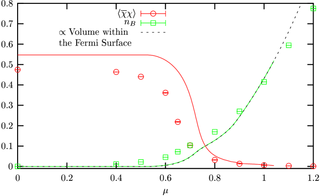
Figure 1: Chiral condensate and number density extrapolated to $V^{-1}\to 0$ as functions of $\mu$, showing both the large-$N_{c}$ solution (solid curve) and lattice results (points). The dashed curve is proportional to the volume of the Brillouin zone bounded by the large-$N_{c}$ Fermi surface.

At $\mu=0$, the large-$N_{c}$ solution predicts a non-zero condensate and zero baryon density, corresponding to a vacuum with broken chiral symmetry. As $\mu$ is increased the system passes into a phase in which chiral symmetry is approximately restored and matter begins to build up, with a pronounced “kink” at $\mu_{c}\simeq 0.75$. In particular, $n_{B}$ is seen to be closely related to the volume of momentum space enclosed by the Fermi surface defined by the Fermi momentum $\vec{k}_{F}$ given for free fermions by

$$\sinh^{2}\mu=\sum_{i=1}^{3}\sin^{2}{k_{Fi}}+\Sigma^{2}$$ (25)

and plotted in the large-$N_{c}$ limit as the dashed line. This implies that in the continuum $n_{B}\propto k_{F}^{3}$ as one would expect, whilst on a lattice $n_{B}$ saturates at the value 1.0 as $\mu\to\infty$.

The lattice data agree qualitatively with our analytic solution, although for these data both $\left<\overline{\chi}\chi\right>$ and $\mu_{o}$ are roughly 15% smaller, an effect we attribute to ${O}(1/N_{c})$ corrections. The transition at $\mu\sim\mu_{c}$ has the appearance of a crossover, and may thus be compatible with a second order transition in the chiral limit $m\to 0$. If this is the case the region with $n_{B}>0$ for $\mu<\mu_{c}$ could be associated with a “nuclear matter” phase, since if, as $T\to 0$, $\Sigma$ falls below its vacuum value $\Sigma_{0}$ for $\mu<\mu_{c}$, the only possible physical agency is $n_{B}>0$ (a mixed phase of quark matter droplets in vacuum at constant pressure is not consistent with thermodynamic equilibrium unless there are at least two conserved quantum numbers present Glendenning (1992)). This behaviour is in marked contrast with that of the 2+1$d$ model in which the transition is strongly first-order and baryonic matter has chiral symmetry restored at any density Hands and Morrison (1999); Hands et al. (2002); Kogut and Strouthos (2001). Finally, it is illustrative to convert these densities into physical units. The large-$N_{c}$ estimate $a^{-1}=720$MeV translates the lattice point $(\mu a,n_{B}a^{3})\simeq(0.65,0.072)$ into $\mu=470$MeV, $n_{B}=3.5\mbox{fm}^{-3}$. Bearing in mind that due to species doubling, in a cube of volume $(2a)^{3}$ $\chi$ describes two spin and four color components of a continuum fermion, we deduce a total physical density of $0.88N_{c}N_{f}\mbox{fm}^{-3}$, to be compared with the nuclear matter onset $\mu_{q}\simeq 320$MeV, $n_{q}\simeq 0.15N_{c}\mbox{fm}^{-3}$.

III.2 Diquark Condensation

The main purpose of this study is to determine the nature of the high density phase in which chiral symmetry is approximately restored. In particular, in order to explore the possibility of a U(1)_B-violating BCS phase, we study the diquark order parameters (12) and their susceptibilities (14) as functions of chemical potential. On their own, the susceptibilities are of limited importance. In conjunction with the Ward identity (15) however, their ratio

$$R=-\frac{\chi_{+}}{\chi_{-}}$$ (26)

provides an important tool to distinguish between phases in which U(1)_B symmetry is either manifest or broken. With manifest symmetry, and in the limit $j\to 0$, these two susceptibilities should be identical up to a sign factor, and the ratio should equal 1. If the symmetry is broken, however, the Ward identity predicts that the Goldstone mode $\chi_{-}$ should diverge as $j\to 0$ and hence $R$ should vanish.

As stated in Sec. II.4, the disconnected terms of (14) are calculated via the use of multiple noise vector estimation, whilst the symmetry constraints discussed after (16) imply that the connected terms are given by

$$\chi^{con}_{\pm}=\frac{1}{4}\left(-\left[\left|{\cal G}_{11}\right|^{2}+\left|{\cal G}_{21}\right|^{2}+\left|{\cal G}_{33}\right|^{2}+\left|{\cal G}_{43}\right|^{2}\right]\pm\left[\left|{\cal G}_{13}\right|^{2}+\left|{\cal G}_{23}\right|^{2}+\left|{\cal G}_{31}\right|^{2}+\left|{\cal G}_{41}\right|^{2}\right]\right),$$ (27)

evaluated between a random point source and the point $x$.

The susceptibilities are measured and $R$ calculated on the aforementioned lattice sizes and for various values of $\mu$, with the diquark source $j$ varying from 0.1 to 1.0 during each set of measurements. It is interesting to note that although in most cases the disconnected contributions are found to be consistent with zero, in the low $\mu$ phase with large $j$, $\chi_{+}^{dis}$ can be up to 10-20% the magnitude of $\chi_{+}^{con}$. In contrast with the NJL model in 2+1$d$ Hands et al. (2002), therefore, we cannot assume that $\chi_{+}\simeq\chi_{+}^{con}$.

An interesting empirical observation is that whilst the observables measured in Sec. III.1 were found to scale linearly with the inverse volume of the lattice, observables in the diquark sector appear to scale linearly with the inverse temporal extent, corresponding to the temperature of the system. Accordingly, the ratio $R$ is extrapolated linearly to the limit $L_{t}^{-1}\to 0$, which as in Hands et al. (2002) is found to give a reasonable description of the data. An example of the quality of the fits is illustrated in Fig. 2.

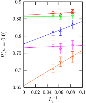
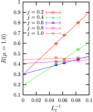
Figure 2: Susceptibility ratio $R$ at $\mu=0.0$ and 1.0 on various lattice sizes.

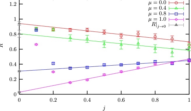
Figure 3: $R$ extrapolated to $j\to 0$ for various values of $\mu$.

Figure 3 shows this extrapolated data plotted as a function of $j$ for various values of $\mu$, as well as the results of a linear extrapolation to $j\to 0$. One immediately notices that whilst this extrapolation appears plausible for $j\geq 0.3$, the data at lower values of $j$ in the high $\mu$ phase diverge rapidly from the linear trend. The fact that this effect increases systematically with increasing $\mu$ and decreasing $j$ suggests that its origin is some systematic effect not considered thusfar; indeed, the study presented in Sec. VI shows this to be due to residual finite temperature effects. For this reason, we believe that we are justified in disregarding data with $j\leq 0.2$ when taking the $j\to 0$ limit. With this omission Fig. 3 shows that for $\mu=0$ a linear fit is consistent with a ratio of $R\approx 1$, corresponding to a manifest baryon number symmetry as one would expect in the vacuum. At $\mu=1.0$, however, $R\approx 0$ suggesting that U(1)_B symmetry is broken.

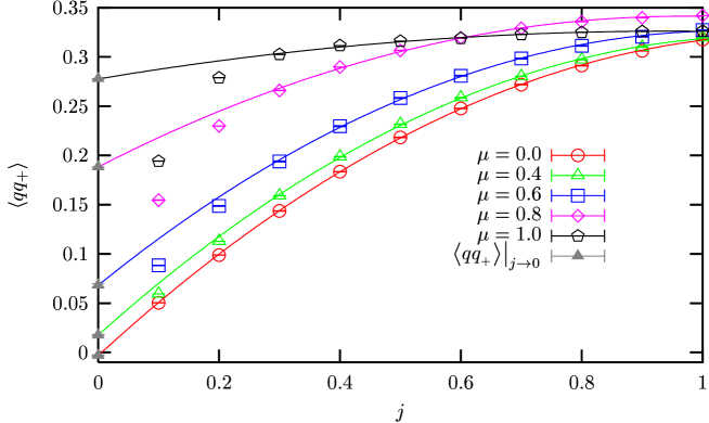
Figure 4: $\left<qq_{+}\right>$ extrapolated to $j\to 0$ for various values of $\mu$.

For more direct evidence of diquark condensation we measure the order parameter defined in (12). Again, these data are extrapolated linearly to the limit $L_{t}^{-1}\rightarrow 0$ with the quality of the fits being good. Figure 4 shows the extrapolated values of $\left<qq_{+}\right>$ plotted against $j$ for various values of $\mu$. Fitting a quadratic curve through the data with $j\geq 0.3$, one can clearly see that the high $\mu$, low $j$ data again disagree with the curve; again ignoring these points, the data are extrapolated to $j\to 0$. For $\mu=0$ we find no diquark condensation as one would expect, but as $\mu$ increases from zero, so does $\left<qq_{+}\right>$. Together, the observations that $\lim_{j\to 0}R=0$ and $\lim_{j\to 0}\langle qq_{+}\rangle\not=0$ support the existence of a BCS superfluid phase at high chemical potential.

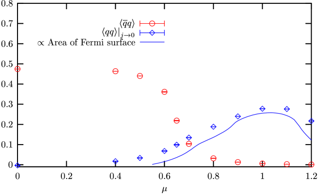
Figure 5: A comparison between the diquark and chiral order parameters as functions of $\mu$.

Finally, $\left<qq_{+}\right>$ is plotted as a function of $\mu$ in Fig. 5, along with the previously presented result for $\left<{\overline{\chi}}\chi\right>$. Although there is clearly a transition from a phase with no diquark condensation to one in which the diquark condensate has a magnitude similar to that of the vacuum chiral condensate, this transition is far less pronounced than in the chiral case. $\left<qq_{+}\right>$ increases approximately as $\mu^{2}$, but eventually saturates as $\mu$ approaches 1.0 and even decreases past $\mu\sim 1.1$. This behaviour is directly related to the geometry of the Fermi surface for a system defined on a cubic lattice, the area of which we have calculated in the large-$N_{c}$ free fermion limit from (25) and have plotted as the solid curve. The method of this calculation is sketched in Appendix A. In the continuum, $\left<qq_{+}\right>$ should continue to rise as $\mu^{2}$, such that the curvature $\partial^{2}\left<qq_{+}\right>/\partial\mu^{2}$ is positive, in contrast to the behaviour observed in simulations of two color QCD, in which there is no Fermi surface and U(1)_B breaking proceeds via Bose-Einstein condensation Aloisio et al. (2001); Kogut et al. (2003); Hands et al. (2001b) leading to $\partial^{2}\langle qq_{+}\rangle/\partial\mu^{2}<0$.

The apparent weakness of the transition at intermediate $\mu$ is related to the fact that at these chemical potentials, the value of $\left.R\right|_{j\to 0}$ interpolates between the two extremes of 0 and 1. This is counterintuitive, since it suggests a partially broken symmetry, even at $j=0$. It may be that this is a side-effect of the chiral transition being a crossover, since there is no sharp point at which a large Fermi surface is created. It is also possible, of course, that this behaviour for intermediate $\mu$ is merely an artifact of our poor control over the $j\to 0$ extrapolation.

IV The Quasiparticle Dispersion Relation

IV.1 Spectroscopy in the Fermionic Sector

In this section we study the dynamics of the model’s fermionic excitations, which as in the original BCS theory Bardeen et al. (1957) can be viewed as quasiparticles with energy $E$ relative to the system’s Fermi energy $E_{F}$. In a traditional Fermi liquid, these can be identified with particle excitations above the Fermi surface, and hole excitations below, both of which can have energies arbitrarily close to $E=0$. In a superfluid system, however, the particles and holes mix, and energies of the lowest-lying excitations are separated from zero by a BCS gap $\Delta$, which in analogy to the chiral mass gap in the vacuum $\Sigma_{0}$, can be viewed as an effective order parameter for the system. One advantage of this parameter is that unlike the diquark condensate, $\Delta$ can be directly related to a macroscopic thermodynamic property of the system, the critical temperature $T_{c}$ Schmitt et al. (2002). In principle, being a spectral quantity it is also measurable in a color superconducting phase in QCD, where according to Elitzur’s theorem one cannot define a local order parameter in a gauge invariant way Elitzur (1975).

The propagation of the quasiparticles is described by the Gor’kov propagator, defined in (16), such that by analysing its momentum dependence we can map out a quasiparticle dispersion relation $E(k)$, i.e. the energy spectrum as a function of momentum, and hence measure $\Delta$. In particular, we have measured the time-slice form of both “normal” and “anomalous” propagators

$$N(\vec{k};t)=\sum_{\vec{x}}{\rm Re}\left[\bar{N}_{11}(\vec{0},0;\vec{x},t)\right]e^{-i\vec{k}.\vec{x}};$$ (28)

$$A(\vec{k};t)=\sum_{\vec{x}}{\rm Im}\left[A_{12}(\vec{0},0;\vec{x},t)\right]e^{-i\vec{k}.\vec{x}},$$ (29)

on $L_{x}\times L_{y,z}^{2}\times L_{t}$ lattices with $L_{x}=96$, $L_{y,z}=12$. This choice of having one spatial direction much longer than the others gives the system a large number of modes with which to sample $E(k)$, whilst minimising the extra computational expense of running on a larger volume. In particular, by setting $\vec{k}=(k,0,0)$ with $k=2\pi n/L_{x}$ $(n=0,1,2,\dots,L_{s}/4)$, the lattice fermions have 25 independent modes between 0 and $\pi/2$ in the $k_{x}$ direction. Since the study presented in Sec. V shows that the diquark observables display little spatial dependence, there should be no detrimental effects from working with $L_{x}\gg L_{y,z}$.

Simulations were performed with $L_{t}=16$ and 20 at various chemical potentials using the same values of the diquark sources as in the previous section. $L_{t}=12$ data were also generated, but these prove to have too few time-slices over which to reliably fit the propagator, and are therefore neglected in our analysis. Again, approximately 500 equilibrated trajectories were generated per run, with measurement taking place on every other configuration. Two additional simulations were performed at $\mu=0.0$ and 0.8 with $L_{t}=24$, which after equilibration took approximately $5\frac{1}{2}$ and $16$ CPU days respectively to generate 400 trajectories on a 2.0GHz Intel Xeon processor.

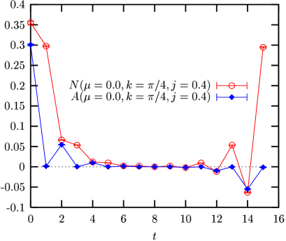
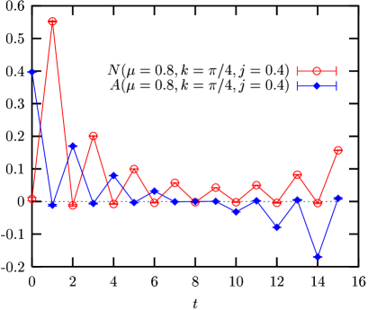
Figure 6: Normal and anomalous propagators measured on a $96\times 12^{2}\times 16$ lattice in both the chirally broken and restored phases.

Some example propagators in both the chirally broken and restored phases are plotted in Fig. 6. At $\mu=0.0$ the normal propagator is non-zero for all $t$, whilst at $\mu=0.8$ it approximates zero on even time-slices, which reflects the fact that with manifest chiral symmetry the $N_{oo}$ and $N_{ee}$ components of the standard staggered fermion propagator vanish. The anomalous propagator is zero on all odd time-slices for all values of $\mu$.

To map out the dispersion relation for each value of $\mu$, the energy is extracted by fitting the propagators to

$$\begin{array}[]{c l l}N(k,t)=Ae^{-Et}+Be^{-E(L_{t}-t)}&{\rm if}&t={\rm odd}\\ N(k,t)=0&{\rm if}&t={\rm even}\end{array}$$ (30)

and

$$\begin{array}[]{c l l}A(k,t)=C(e^{-Et}-e^{-E(L_{t}-t)})&{\rm if}&t={\rm even}\\ A(k,t)=0&{\rm if}&t={\rm odd},\end{array}$$ (31)

where $A$, $B$ and $C$ are kept as free parameters, as is the energy $E$. Although, as expected, the values of $E$ extracted from the two propagators are found to be consistent, we choose to use those extracted from (31) to map out our dispersion relation, since having one less free parameter than (30), the fits to this form are found to be of a higher quality. Some example fits are illustrated in Fig. 7.

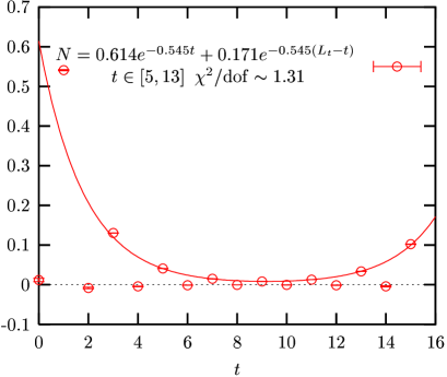
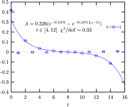
Figure 7: Normal and anomalous propagators with $j=0.3$ and $k=\pi/4$ with their fitted curves measured on a $96\times 12^{2}\times 16$ lattice at $\mu=0.8$.

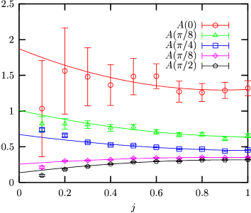
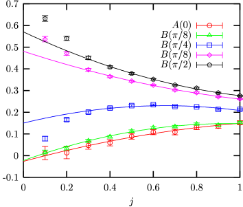
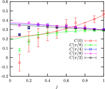
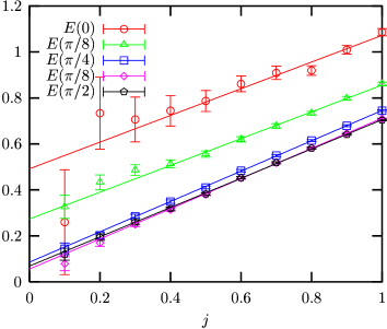
Figure 8: Zero temperature propagator parameters at $\mu=0.8$ and various values of $k$. The solid curves show extrapolation to $j\to 0$.

Figure 8 shows plots of the free parameters in (30) and (31) at $\mu=0.8$, extrapolated to $T\to 0$; in turn these are extrapolated to $j\to 0$. Quadratic polynomial curves are fitted to the coefficients $A(k)$, $B(k)$ and $C(k)$, whilst the energy $E(k)$ is fitted linearly. As with the extrapolations of $\left<qq_{+}\right>$ and $R$, these appear to smoothly fit the data except for those with low values of the diquark source $j$, for which the discrepancy discussed in Sec. III.2 persists. Again, points with $j<0.3$ are ignored for the purpose of the extrapolations; we rely on the conclusions of Secs. V and VI to justify the omission of these data from our analysis.

IV.2 The Vacuum Dispersion Relation

Before considering a lattice system with a Fermi surface, we review the nature of the dispersion relation in the familiar case of the vacuum. With $\mu=0$, time reversal is a good symmetry of the lattice and the coefficients $A$ and $B$ become identical such that (30) reduces to its usual form $\left|N(k,t)\right|=A(e^{-Et}+e^{-E(L_{t}-t)})$. This can be understood physically by noting that the vacuum spectrum appears identical to both particles and antiparticles, and hence to both the forward- and backward-moving parts of $N$. In agreement with this, $A$ and $B$ are found to be equal, within errors, for all three values of $L_{t}$.

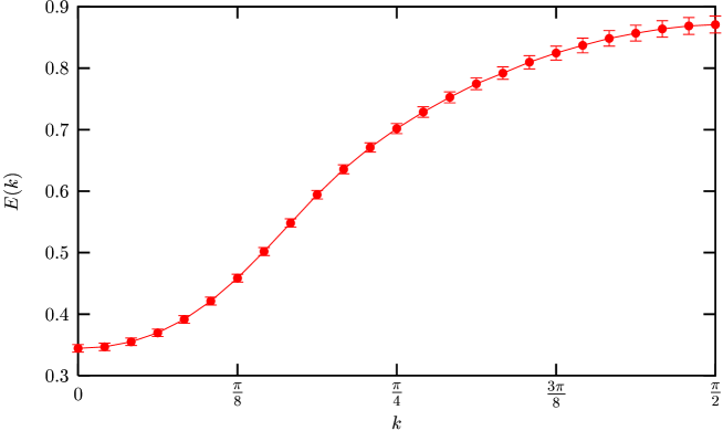
Figure 9: The vacuum dispersion relation $E(k)$ extrapolated to $T\to 0$ and then $j\to 0$.

Figure 9 illustrates the energies extracted from $A(k,t)$, extrapolated to zero temperature through $L_{t}=16$, 20 and 24 and then to $j\to 0$, which results in the familiar lattice dispersion relation $E(k,\mu=0)$ Boyd et al. (1992)

$$\sinh^{2}E=\alpha^{2}\sum_{i=1}^{3}\sin^{2}k_{i}+\Sigma_{0}^{2},$$ (32)

where $\alpha$ is a constant which allows for the renormalisation of the speed of light by thermal effects; in practice its fitted value is close to one as expected. The energy gap at $k=0$ can be identified with the vacuum fermion mass, from which we learn that $\Sigma_{0}=0.351(6)$. As $k$ is increased, the dispersion relation is approximately quadratic for small $k/\Sigma_{0}$ (as expected for a non-relativistic particle), until discretisation effects dominate its form and the periodicity of (32) causes it to level off as $k\to\pi/2$.

IV.3 Measurement of the Gap

In this section we study the dispersion relation at $\mu=0.8$, with the aim of observing the BCS gap $\Delta$. First, however, we study the momentum dependence of the other free parameters fitted from the forms (30) and (31). Figure 10 illustrates the values of $A$, $B$ and $C$ extrapolated first to $T\to 0$ and then to $j\to 0$, and plotted as functions of momentum $k$.

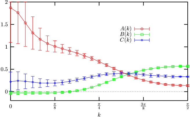
Figure 10: The propagator coefficients $A$, $B$ and $C$ for $\mu=0.8$ extrapolated to $T\to 0$ and then $j\to 0$.

The coefficients $A(k)$ and $B(k)$ represent the amplitudes of forward- and backward-moving spin-$\frac{1}{2}$ propagation, which due to our choice to study the antiparticle propagator $N\equiv\overline{N}_{11}={\cal G}_{31}\sim\left<\overline{q}(x)q(y)\right>$, correspond to hole and particle excitations respectively in the limit that $j\to 0$. For small momenta, corresponding to excitations deep within the Fermi sea, propagation is dominated by hole degrees of freedom. As the Fermi momentum is approached, particles are easier to excite and become the dominant contribution as $k\to\frac{\pi}{2}$. To degrees of freedom with $k=k_{F}$, as in the vacuum the background appears the same to both particles and holes such that $A(k_{F})=B(k_{F})$. For this reason, in analogy with the coefficients of filled and unfilled states in the original BCS theory Bardeen et al. (1957), the intercept of the curves of $A(k)$ and $B(k)$ defines the Fermi momentum for the interacting theory in the $T\to 0$ limit. In the anomalous sector, the coefficient $C(k)$ is approximately zero deep within the Fermi sea, but becomes non-zero (even in the limit $j\to 0$) in a broad peak about the Fermi momentum, which is a sign of particle-hole mixing in this region. This is in contrast with similar measurements in NJL₂₊₁ Hands et al. (2002).

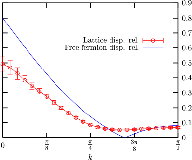
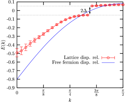
Figure 11: The lattice dispersion relation and typical free fermion dispersion relation at $\mu=0.8$. In the right-hand panel the hole branch is plotted as negative.

The left-hand panel of Fig. 11 illustrates the lattice dispersion relation $E(k)$ at $\mu=0.8$ extracted from (31) and extrapolated first to $T\to 0$ and then $j\to 0$ (points), compared with that of free massless fermions on the lattice, parametrised by

$$E(k)=-\mu+\sinh^{-1}(\sin k).$$ (33)

For this free dispersion relation, there are two distinct branches, one for hole excitations below the Fermi surface for which $E$ reduces with $k$, and one for particle excitations for which $E$ increases with $k$. We should note at this point that the crossover between these regimes, $k_{F}=\sin^{-1}(\sinh 0.8)\sim 0.348\pi$, is consistent with the intercept of $A(k)$ and $B(k)$ in Fig. 10 to within the precision allowed by the momentum resolution. By contrast the lattice data display no evidence for two distinct branches, which is another signal of particle-hole mixing. More importantly, at no point do the lattice data pass through zero, but between $\pi/3\leq k\leq 17\pi/48$ (again consistent with the free-field $k_{F}$), they have a minimum of $E(k)=0.053(6)$; this is the BCS gap $\Delta$. Comparing this to our measurement of the vacuum fermion mass in Sec. IV.2, we find the ratio

$$\frac{\Delta(\mu=0.8)}{\Sigma_{0}}=0.15(2),$$ (34)

which assuming a fermion mass of 400${\rm MeV}$ implies that $\Delta(\mu=0.8)\sim 60{\rm MeV}$, consistent with the analytic predictions of Berges and Rajagopal (1999); Nardulli (2002).

This may be viewed more graphically in the right-hand panel of Fig. 11, where excitations below $E_{F}$ have been plotted as negative. This makes the free fermion dispersion relation a smooth curve that passes continuously through $E=0$ at the Fermi momentum, and is similar in nature to that of lattice four-Fermi models with no BCS gap Hands et al. (2002, 2003). For our data, however, this plot introduces a discontinuity of $2\Delta$ which looks exactly like that of a traditional BCS superfluid in the continuum.

IV.4 $\mu$ Dependence of the Gap

Having systematically investigated the dispersion relation and extracted the gap at one value of chemical potential, it would be illuminating to repeat the analysis of the previous section for a range of chemical potentials in the BCS phase. However, generating data with $L_{t}=24$ in the chirally restored phase is a CPU intensive task, taking $O$(20) CPU days on a fast desktop PC for each value of $\mu$. The reason this is so much more expensive than in the chirally broken phase is that the rate of convergence of the conjugate gradient subroutine used to invert $M^{\dagger}M$ in the generation of our $\{\Phi\}$ configurations is related to the magnitude of the diagonal components of $M$, which are in turn proportional to the constituent quark mass $\Sigma(\mu>\mu_{c})\simeq 0$.

For this reason we utilise the data generated with $L_{t}=16$ and 20 and approximate the $T\to 0$ limit by extrapolating through these data and assigning a conservative estimate for the error; the $j\to 0$ extrapolations may then be carried out as before. Although of little statistical significance, it should be noted that the dispersion relation at $\mu=0.8$ extracted using this method is consistent, for all values of $k$, with that extracted using the full statistical treatment of the previous section.

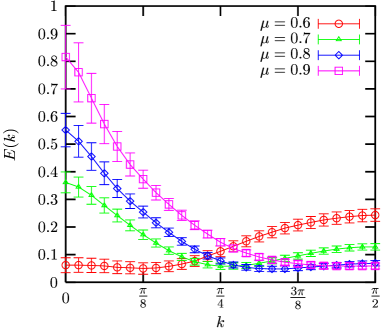
Figure 12: Lattice dispersion relations at various values of $\mu$.

Figure 12 illustrates a selection of these dispersion relations for various chemical potentials. An interesting point to note is that unlike the diquark condensate, there is an upper bound of $\mu\sim\sinh^{-1}(1.0)\sim 0.88,$ above which we cannot extract an estimate of the gap using the method outlined in Sec. IV.1. This can be understood by considering the nature of the lattice Fermi surface for free fermions in the infinite volume limit, parametrised by (25) and plotted at two values of $\mu$ in the large-$N_{c}$ limit in Fig. 13.

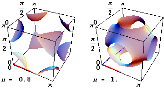
Figure 13: The zero temperature, infinite volume Fermi surface at two values of chemical potential.

For ${k_{F}}_{i}\ll\pi/2$, corresponding to small values of $\mu$, the small-angle identities imply that the surface is approximately spherical and the momenta sampled herein, emphasised on the $k_{x}$ axis in Fig. 12, are sufficient to probe either side of the surface and detect the presence of a gap. For $\mu>\sinh^{-1}(\sin{\pi/2})$, however, the reduced rotational invariance of the lattice dominates, and (25) has no real solution with $\vec{k}=(0\leq k_{x}\leq\frac{\pi}{2},0,0)$. It is for this reason that the curve at $\mu=0.9$ in Fig. 12 shows no minimum and we cannot extract a value of $\Delta$. Whilst there is almost certainly a gap present, as the maximum of $\left<qq_{+}\right>$ lies between $1.0\leq\mu\leq 1.1$, to detect its presence via the dispersion relation one is required to sample momenta along e.g. the more complicated diagonal path $\vec{k}=(k,k,k)$ with $0\leq k\leq\pi/2$, illustrated in the right-hand panel of Fig. 13. Because of the large number of spatial modes required to sample this path with sufficient resolution, such a study is computationally beyond our current capability.

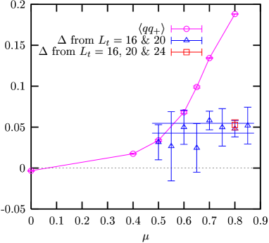
Figure 14: Estimates for the gap $\Delta$ compared with $\left<qq_{+}\right>$ for a range of $\mu$.

Finally, $\Delta$ is plotted as a function of $\mu$ in Fig. 14 and compared with the value of the diquark condensate. Although the error bars on our estimated values are fairly large, we see little evidence of any $\mu$ dependence once the gap becomes non-zero. In fact, a least-squares fit to $\Delta={\rm constant}$, denoted by the horizontal bar, has a chi-squared value of only 0.33 per degree of freedom. In combination with Fig. 5, Fig. 14 provides qualitative support for a simple-minded picture in which only diquark pairs within a shell encasing the Fermi surface of thickness $2\Delta$, independent of $\mu$, participate in the pairing, resulting in a condensate $\langle qq_{+}\rangle\propto\Delta\mu^{2}$.

V Finite Spatial Volume Effects

The conclusions of Secs. III and IV, that the high-$\mu$ phase is one with both $\left<qq_{+}\right>\neq 0$ and $\Delta\neq 0$, both rely on the discarding of data with $j<0.3$, since results in the diquark sector with these small diquark sources disagree with the trends at higher $j$. In order to be able to trust our $j\to 0$ extrapolations it is necessary, therefore, to justify this omission, especially since it is the data in the region of this limit that have been discarded.

We have previously argued that the discrepancy at low-$j$ could be due to finite size effects Hands and Walters (2002), since whilst our simulations were performed on lattices with $L_{s}\lesssim 20$, variational studies of the $N_{f}=2$, $N_{c}=3$ continuum NJL model at zero temperature in a finite spatial volume show that with no diquark source, a spatial extent of 7fm ($\sim 25$ lattice spacings) is required before the model approximates its infinite volume limit Amore et al. (2002). We have argued further that the source of these finite size effects is due not to the realisation of an exact Goldstone-mode, but to the difficulty of representing a thin shell of states about the Fermi surface which contribute to diquark condensation on a discrete momentum lattice. Whilst this is supported in part by the finite size study presented in Hands and Walters (2002), in which $\left<qq_{+}\right>$ displays a non-monotonic dependence on $L_{s}$, it should be noted that the magnitudes of these fluctuations are less than 1% for $L_{s}\geq 8$ and all values of $j$, much smaller than the approximate $30\%$ suppression of $\left<qq_{+}\right>$ at $j=0.1$ seen in Fig. 4. In fact, the diquark condensate shows little notable $L_{s}$ dependence even prior to extrapolation to $T\to 0$.

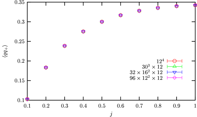
Figure 15: Diquark condensate at $\mu=0.8$ on $L_{x}\times L_{y,z}^{2}\times L_{t}$ lattices with $L_{t}=12$ and various $L_{x,y,z}$.

In Fig. 15, $\left<qq_{+}\right>$ is plotted as a function of $j$ at $\mu=0.8$ with $L_{t}=12$ and various spatial extents, including the results of a large simulation with $L_{s}=30$. This shows that the diquark condensate displays no significant size dependence at any $j$. The same lack of any significant spatial size dependence is found for both $\left<qq_{+}\right>$ with $L_{t}=16$ and 20 and for $E(k)$ with $L_{t}=16$ and 20 within the allowed momentum resolution. The fact that these observables remain unchanged at low $j$, even when changing the spatial volume by up to a factor of $2.5^{3}\sim 16$, makes it hard to believe our previous suggestion that the suppression at $j<0.3$ is due to finite size effects. Instead, we propose an alternative suggestion in the following section.

VI Non-zero Temperature

In previous reports of this work Walters and Hands (2004); Walters (2003), we have suggested that an obvious extension would be to carry out simulations at non-zero temperature, with the aim of measuring the critical temperature of the superfluid phase, $T_{c}$. The non-relativistic BCS theory predicts the relation between this parameter and the magnitude of the gap to be Bardeen et al. (1957)

$$\frac{\Delta}{T_{c}}=1.764.$$ (35)

Furthermore, it has been shown that this relation holds for relativistic color superconducting systems in weakly coupled QCD with two flavors Schmitt et al. (2002). Although such weak coupling predictions may be trusted only at asymptotically high densities, naïvely applying (35) to our measurement of $\Delta(\mu=0.8)=0.053(6)$ suggests that $T_{c}\sim 0.03a^{-1}$, such that at this chemical potential and in the limit $j\to 0$, one should observe a superfluid phase only when the temporal extent is greater than about 35 lattice spacings. The fact that we observe a BCS phase, even though our simulations were performed on lattices with temporal extents much smaller than this relies on our performing measurements with $j\neq 0$ and then extrapolating in the correct manner. Setting $j\neq 0$ has the effect of making condensation more favourable, which suggests that at fixed $j$ there could be a crossover at some pseudo-critical temperature, $T_{c}(j)$, separating a region where diquark condensation is suppressed by thermal fluctuations and one in which it is not. One would expect the effect of increasing the source would be to increase $T_{c}(j)$ such that diquark condensation can be observed on lattices with smaller temporal extents. If one can successfully extrapolate to zero temperature first, a $j\to 0$ extrapolation should then be possible.

This causes a problem if one wishes to determine the value of the condensate at a particular chemical potential and non-zero temperature, since it is possible that at temperatures close to $T_{c}$, $T_{c}(j)$ crosses the temperature of the lattice over the range of $j$ studied. Figure 16 illustrates the diquark condensate measured at $\mu=0.8$ on lattices with various temporal extents corresponding to various non-zero temperatures, as well as the “$T=0$” curves for $\mu=0.0$ and 0.8 from $12^{4}$, $16^{4}$ and $20^{4}$ lattices, as plotted in Fig. 4.

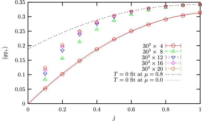
Figure 16: Diquark condensate at $\mu=0.8$ on various lattices at non-zero temperature.

The $L_{t}=4$ results lie well below the $T=0$ curve for all values of $j$, suggesting that the temperature is high enough to suppress condensation for the entire range of $j$. A quadratic extrapolation through these points is very similar to the zero temperature vacuum fit from Fig. 4 and is consistent with $\left.\left<qq\right>\right|_{j\to 0}=0$. As the temperature of the lattice is decreased, however, the data at higher $j$ are no longer suppressed and an extrapolation through all $j$ is no longer possible. This can be seen more clearly in Fig. 17, where we focus on the data measured on a $30^{3}\times 12$ lattice.

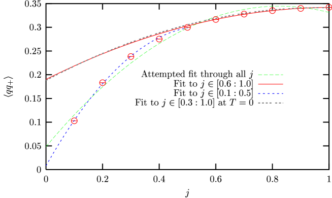
Figure 17: Diquark condensate at $\mu=0.8$ an a $30^{3}\times 12$ lattice.

Whilst an attempted fit through all values of $j$ appears of poor quality, by choosing a suitable point to separate the low- and high-$j$ data one can fit the two regions successfully.

Whilst this implies that establishing the critical temperature of the superfluid phase is not as simple as we initially believed, it does provide an alternative explanation of the suppression in $\left<qq_{+}\right>$ at $T=0$ for $j<0.3$. The fact that the curve fitted through the $L_{t}=12$ data over $j\in[0.6:1.0]$ agrees with that of data extrapolated to $T\to 0$ and fitted over $j\in[0.3,1.0]$ suggests that these curves represent not the correct infinite volume limit, as previously suggested, but the correct zero temperature limit of the $j\to 0$ extrapolation. Whilst a linear $T\to 0$ extrapolation is sufficient to reach this curve for $0.3\leq j\leq 0.5$, the data at $j<0.3$ must be suppressed too much for such an extrapolation to be sufficient, i.e. the temperature of the lattice must be too high compared with $T_{c}(j<0.3)$. This justifies in retrospect the discarding of the low $j$ data in the extrapolations of Secs. III and IV, which form the basis for the claimed superfluid ground state.

VII Non-zero Isospin Chemical Potential

In previous sections, we have demonstrated numerically that the ground-state of our two flavor model at non-zero $\mu$ and low $T$ is that of a BCS gapped lattice superfluid. The pairing mechanism in this system, between quarks of opposite momenta and isospin, and thus analogous to 2SC condensation between $u$ and $d$ quarks in QCD, is particularly energetically favourable. If the system were non-interacting, it would cost no energy to create a pair of quarks at the common Fermi surface of the degenerate flavors, such that when the attractive interaction is restored, the system is expected always to be unstable to diquark condensation Alford et al. (2001b).

In nature, however, the Fermi momenta $k_{F}^{u}$ and $k_{F}^{d}$ for up and down quarks respectively are expected to differ. A simplistic argument outlined in Alford et al. (2000), simplified still further here to describe a two flavor system, suggests that in compact stellar matter $k_{F}^{u}$ should be less than $k_{F}^{d}$. For massless non-interacting matter with baryon chemical potential $\mu_{B}=400{\rm MeV}$, an electron chemical potential $\mu_{e}=89{\rm MeV}$ is required to enforce both charge neutrality and chemical equilibrium under weak interactions. Together, these two conditions determine all the chemical potentials and Fermi momenta:

$$\begin{array}[]{c}k_{F}^{u}=\mu_{u}=\mu_{B}-\frac{1}{2}\mu_{e}=355.5{\rm MeV},\\ k_{F}^{d}=\mu_{d}=\mu_{B}+\frac{1}{2}\mu_{e}=444.5{\rm MeV},\\ k_{F}^{e}=\mu_{e}=89{\rm MeV}.\end{array}$$ (36)

Here we use the term baryon chemical potential in the context of the NJL model, where baryons are identified with quarks and $\mu_{B}\equiv\frac{1}{2}(\mu_{u}+\mu_{d})$. The effect of separating the free-particle Fermi surfaces of pairing quarks should be to make the superconducting phase less energetically favourable, and should prove a good method to investigate the stability of the superfluid phase.

Such a study was applied to the 2SC color superconducting phase in a mean field four-Fermi model in Bedaque (2002). Similar to results for superconductors in the presence of a magnetic field Clogsten (1962); Chandrasekhar (1962), when the free field Fermi surfaces are separated by only a small amount the ground-state of interacting matter remains superconducting with degenerate Fermi surfaces for the pairing partners. At some critical free fermion separation, however, the system is found to go through a first order transition to a gapless Fermi liquid with two separate surfaces. Unlike normal superconductors, however, the size of the gap increases slightly under small flavor asymmetries, an effect attributed to the model’s color structure extracted from one gluon exchange in QCD. This analysis has also been extended further to include systems in which the Fermi surfaces $k_{F}^{u}$ and $k_{F}^{d}$ are separated not only by an isospin chemical potential, but a fixed momentum $\vec{q}$ Alford et al. (2001b). In such a system, when $\left|k_{F}^{u}-k_{F}^{d}\right|$ and $\vec{q}$ are sufficiently large that the Fermi surfaces cross, Pauli blocking implies that 2SC becomes unstable with respect to a state in which diquark condensation occurs only at a ring of states close to the intercept of the surfaces. The state has both broken translational and rotational invariance in which the diquark pairs have non-zero total momentum; in analogy with such phases in electron superconductivity this is known as the LOFF phase Larkin and Ovchinnikiv (1964); Fulde and Ferrel (1964).

In the lattice NJL model, the pairing quarks of opposite isospin are represented by the two components of the staggered fermion field

$$\chi_{x}\equiv\left(\begin{array}[]{c}\chi_{1}(x)\\ \chi_{2}(x)\end{array}\right)=\left(\begin{array}[]{c}u(x)\\ d(x)\end{array}\right),$$ (37)

hereon referred to as “up” and “down” quark flavors. The Fermi surfaces of the pairing partners can be separated by directly allocating them different chemical potentials, $\mu_{u}$ and $\mu_{d}$, equivalent to having simultaneously non-zero baryon chemical potential $\mu_{B}=\frac{1}{2}\left(\mu_{u}+\mu_{d}\right)$ and isospin chemical potential $\mu_{I}=\frac{1}{2}\left(\mu_{u}-\mu_{d}\right)$. Although this definition implies that $\mu_{u}>\mu_{d}$, which is contrary to the conclusions of the argument outlined above, this notation has been chosen to be consistent with the analytic studies of Toublan and Kogut (2003) and Frank et al. (2003) (since the NJL model does not include weak interactions and is therefore isospin invariant, the labels $u$ and $d$ are interchangeable). In the physical context of compact stars, the two scales should be ordered $\mu_{B}\gg\mu_{I}$, since the simple argument leading to (36) predicts that $\frac{1}{2}\left|\mu_{u}-\mu_{d}\right|\sim 0.1\mu_{B}$.

With this introduction, the fermion kinetic operator $M$, defined previously in (3) becomes

$$M^{pq}_{xy} = \frac{1}{2}\left(e^{\mu_{B}}(e^{\tau_{3}\mu_{I}})^{pq}\delta_{yx+\hat{0}}-e^{-\mu_{B}}(e^{-\tau_{3}\mu_{I}})^{pq}\delta_{yx-\hat{0}}\right)$$

$$+ \frac{1}{2}\delta^{pq}\left[\sum_{\nu=1}^{3}\eta_{\nu}(x)\left(\delta_{yx+\hat{\nu}}-\delta_{yx-\hat{\nu}}\right)+2m\delta_{xy}\right]$$

$$+ \frac{1}{16}\delta_{xy}\sum_{\left<\tilde{x},x\right>}\left(\sigma(\tilde{x})\delta^{pq}+i\epsilon(x)\vec{\pi}(\tilde{x}).\vec{\tau}^{pq}\right).$$

Unfortunately, this means that the proof that $\det M$ is real and positive presented in Hands et al. (2002) is no longer valid, which can be seen be noting that e.g. $\tau_{2}(e^{\tau_{3}\mu_{I}})\tau_{2}=e^{-\tau_{3}\mu_{I}}\neq(e^{\tau_{3}\mu_{I}})^{*}$, and the identity $\tau_{2}M\tau_{2}=M^{*}$ no longer holds. Although this would not cause the simulation to fail, since we use $\det M^{\dagger}M$ as our fermionic measure, the fact that this choice is the sole reason the algorithm would work implies that non-trivial interactions between $\chi$ and $\zeta$ quarks will be introduced which could cause the argument of Barbour et al. (1999) to break down. Instead, we choose to simulate in the quenched isospin limit in which $\det M^{\dagger}M$ is calculated with $\mu_{I}=0$ in the HMC update of the bosonic fields, whilst (VII) is used in ${\cal A}$ during the measurement of the observables.

Before we discuss setting $\mu_{I}\neq 0$ in the superfluid phase, let us examine the effect this introduction has on the chiral phase transition. An analytic study of the NJL model has shown that introducing a small $\mu_{I}$ causes the chiral phase transition to split into two, one transition for the condensate of each quark flavor Toublan and Kogut (2003).

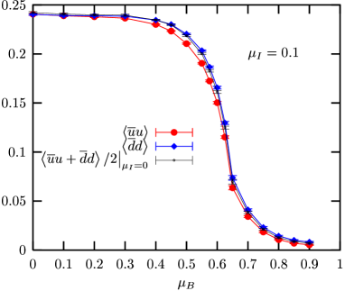
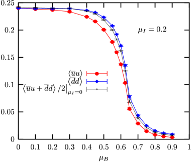
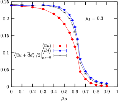
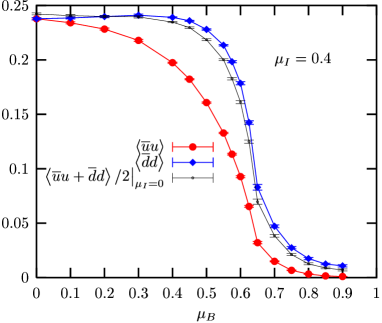
Figure 18: $\left<\overline{u}u\right>$ and $\left<\overline{d}d\right>$ condensates for various $\mu_{B}$ and $\mu_{I}$ on a $12^{4}$ lattice.

Figure 18 illustrates lattice measurements of the up and down quark condensates

$$\left<\overline{u}u\right>,\left<\overline{d}d\right>\equiv\frac{1}{V}\frac{\partial\ln{Z}}{\partial m_{u,d}}=\frac{1}{4V}\left<{\rm tr}\left(\begin{array}[]{c c}&\openone\pm\tau_{3}\\ -\openone\mp\tau_{3}&\end{array}\right){\cal A}^{-1}\right>$$ (39)

as functions of $\mu_{B}$ for various $\mu_{I}$ measured on a $12^{4}$ lattice. Although these results are measured on only one volume, the speed of these simulations means that is is possible to gain fine resolution in $\mu_{B}$. Consistent with the predictions of Toublan and Kogut (2003), the two transitions, which are coincident in the limit that $\mu_{I}\to 0$, separate as $\mu_{I}$ is increased. This can be understood by noting that for fixed $\mu_{I}$ the chemical potential of the up quark is larger than that of the down, such that as $\mu_{B}$ increases, $\mu_{u}$ reaches the critical chemical potential first. It is not clear, however, why the curve of the up condensate deviates from the $\mu_{I}=0$ solutions more than that of the down. This effect, not predicted in Toublan and Kogut (2003), could be some finite volume artifact, or a result of the quenched approximation. As an aside, it has been argued that the observation of two transitions is an artifact of the diagonal flavor structure of the NJL model with broken chiral symmetry and would not be observed in nature. In particular, the introduction of an instanton-motivated flavor mixing vertex with even a weak coupling is shown to restore the single transition Frank et al. (2003).

In the diquark sector, we relabel the order parameter $\left<qq_{+}\right>$ defined in (12) as $\left<ud\right>$, to emphasise the fact that condensation occurs between quarks of different flavors.

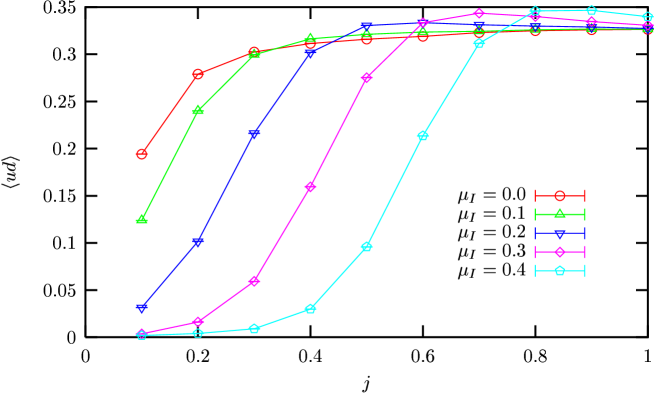
Figure 19: $\left<ud\right>$ condensate as a function of $j$ for various $\mu_{I}$ with $\mu_{B}=1.0$.

Figure 19 illustrates the $\left<ud\right>$ condensate measured at $\mu_{B}=1.0$ on $12^{4}$, $16^{4}$ and $20^{4}$ lattices as a function of $j$ for various values of $\mu_{I}$. Results are extrapolated to $T\to 0$ as before. As expected, the effect of significantly increasing $\mu_{I}$ for fixed $j$ is to suppress condensation, an effect that is more pronounced at smaller values of $j$. Less straightforward to understand, however, is that at values of $j$ above this suppression $\left<ud(j)\right>$ appears to increase slightly with increasing $\mu_{I}$. By analogy with Bedaque (2002), this could be due to the non-trivial $O(a)$ color-mixing terms of the staggered quark action, but again could be due to the crudeness of the quenched approximation.

As with our results at non-zero temperature, because the effect of increasing the diquark source is to make the superfluid more robust to setting $\mu_{I}\neq 0$, it is not yet clear how to determine the critical isospin chemical potential in the limit $j\to 0$.

VIII Summary

To our knowledge this is the first systematic non-perturbative study of a 3+1$d$ relativistic system (albeit one with a Lorentz non-invariant cutoff) which has a Fermi surface. Our goal has been to study such a system with phenomenologically reasonable parameters, but with the main focus on characterising the high-density ground state. The principal result is that in the limit $T\to 0$ the Fermi surface is unstable with respect to condensation of diquark pairs in the scalar isoscalar channel, leading to a ground state characterised by a U(1)_B-violating order parameter $\langle qq_{+}\rangle$. The resulting energy gap $\Delta$ which opens up at the Fermi surface is approximately 15% of the constituent quark mass scale, in good agreement with self-consistent estimates made with similar models in continuum approaches. It seems likely that the model is thus a superfluid described in terms of orthodox BCS theory.

Detailed quantitative agreement with further aspects of the BCS theory, such as the prediction (35) for $T_{c}$, is hard to verify because of practical difficulties in simultaneously probing both $T\to 0$ and $j\to 0$ limits. Finite volume effects in this system are complicated to unravel because of their separate dependencies on $L_{s}$ and $L_{t}$. As described in Secs. V and VI, for the first time we have been able to simulate a sufficiently broad range of $L_{s}$, $L_{t}$ to be able to demonstrate that the apparent suppression of the order parameter for small $j$ is due to our distance from the $L_{t}\to 0$ limit. Note, though, that the ratio $L_{t}/L_{s}$ cannot be made arbitrarily large without introducing artifacts due to discretisation of $k$-space, as shown in Fig. 4 of Hands and Walters (2002). With the bare parameters used in this study we estimate that volumes greater than $40^{4}$ will be needed for quantitative studies of $T_{c}$.

Finally, we have made the first exploratory study of a system with non-zero chemical potentials for both baryon number and isospin, which as described in Sec. VII is a necessary precondition for an accurate description of the conditions prevailing inside a neutron star. It is amusing that the sign problem comes back to bite, restricting us to considering non-zero isospin density in the quenched approximation only. Nonetheless, we have been able to observe the expected suppression of $ud$ pairing at the Fermi surface. Bearing in mind that phenomenology demands $\mu_{I}\ll\mu_{B}$, it is not ruled out that future simulations could successfully unquench isospin by either reweighting or analytic continuation in the small parameter $\mu_{I}/\mu_{B}$, much as the conditions in heavy ion collisions can be accessed by lattice QCD simulations at $\mu_{B}=0$ analytically continued in $\mu_{B}/T$.

Appendix A The Area of the Fermi Surface

In Fig. 5 we plot the area of the Fermi surface in the infinite volume limit as a function of chemical potential $\mu$. Here we outline the method used to produce this curve.

In general, one can calculate the area of any surface $S$ by integrating $\phi=1$ over that surface

$$\mbox{Surface Area}=\int_{S}1{\rm d}\sigma,$$ (40)

where ${\rm d}\sigma$ is an infinitesimal two-dimensional element of $S$. If the $z$-component of that surface is single-valued, one may turn this into a two-dimensional integral in the $x$-$y$ plane

$$\int_{S}1{\rm d}\sigma\simeq\iint_{A}\frac{\delta\sigma}{\delta x\delta y}{\rm d}y{\rm d}y,$$ (41)

where $A$ is the area projected onto $z=0$ and $\delta\sigma$ is the area of a parallelogram tangential to $S$ that projects onto a square of area $\delta x\delta y$. In the limit that $\delta\to\rm d$, $\frac{\delta\sigma}{\delta x\delta y}$ is given by the absolute gradient of $z(x,y)$

$$\left|\nabla z(x,y)\right|=\left|\left(\frac{\partial z}{\partial x},\frac{\partial z}{\partial y},\frac{\partial z}{\partial z}\right)\right|=\sqrt{\left(\frac{\partial z}{\partial x}\right)^{2}+\left(\frac{\partial z}{\partial y}\right)^{2}+1}$$ (42)

and the equality in (41) becomes exact.

In calculating the area of the Fermi surface, we consider the section of momentum space with $0\leq k_{x,y,z}\leq\frac{\pi}{2}$ in which the surface is a single-valued function ${k_{F}}_{z}({k_{F}}_{x},{k_{F}}_{y})$. From (25), we find that the $k_{z}$-component of the Fermi surface for free fermions at fixed $\mu$ is given by

$${k_{F}}_{z}({k_{F}}_{x},{k_{F}}_{y})=\sin^{-1}\sqrt{C-\sin^{2}{k_{F}}_{x}-\sin^{2}{k_{F}}_{y}}$$ (43)

where the constant $C\equiv\sinh^{2}\mu-\Sigma^{2}$ and the value of $\Sigma(\mu)$ is taken from the large-$N_{c}$ solution of the gap equation (17) in the infinite volume limit. The absolute gradient of this function is

$$\left|\nabla{k_{F}}_{z}({k_{F}}_{x},{k_{F}}_{y})\right|=\sqrt{1+\frac{\cos^{2}{k_{F}}_{x}\sin^{2}{k_{F}}_{x}+\cos^{2}{k_{F}}_{y}\sin^{2}{k_{F}}_{y}}{(C-\sum_{i=x,y}\sin^{2}{k_{F}}_{i})(1-C+\sum_{i=x,y}\sin^{2}{k_{F}}_{i})}}$$ (44)

and the surface area is given by

$$\iint_{A}\left|\nabla{k_{F}}_{z}({k_{F}}_{x},{k_{F}}_{y})\right|{\rm d}{k_{F}}_{y}{\rm d}{k_{F}}_{x},$$ (45)

which we evaluate numerically. In setting the limits of integration, we have several cases, determined by the value of $C(\mu)$:

1. For $C\leq 0$, (43) has no real solutions and the surface area is zero. From the definition of $C$ one can see that this corresponds physically to the chemical potential being insufficiently large to allow the existence of a sea of particles with mass $\Sigma$.

2. For $0<C\leq 1$, the approximately spherical surface intercepts the $k_{x}$ and $k_{y}$ axes at $\sin^{-1}\sqrt{C}$ and we have one region of integration.

3. For $1<C\leq 2$, the discretisation of space-time dominates and the surface no longer intercepts the axes. This is the situation depicted in the right-hand panel of Fig. 13. (43) no longer has any real solutions with $\sin^{2}k_{x}+\sin^{2}k_{y}\leq 1$ or $>2$. We must separate our integral, therefore, into two regions.

4. For $2<C\leq 3$, the surface is again approximately spherical, but with the centre at $(\frac{\pi}{2},\frac{\pi}{2},\frac{\pi}{2})$. In this final region, saturation effects are dominant as the surface area of the sphere decreases with increasing $\mu$ until at $C=3$ (i.e. $\mu\sim\sinh^{-1}\sqrt{3}\sim 1.32$) the area reduces to zero and the lattice is saturated with fermions.

The limits of integration are listed in table 2.

$C$	$k_{x}$	$k_{y}$
$\leq 0$	${\rm Area}=0$	n/a
$0:1$	$0:\sin^{-1}\sqrt{C}$	$0:\sin^{-1}\sqrt{C-\sin^{2}k_{x}}$
$1:2$	$0:\sin^{-1}\sqrt{C-1}$	$\sin^{-1}\sqrt{C-1-\sin^{2}k_{x}}:\frac{\pi}{2}$
	$\sin^{-1}\sqrt{C-1}:\frac{\pi}{2}$	$0:\sin^{-1}\sqrt{C-\sin^{2}k_{x}}$
$2:3$	$\sin^{-1}\sqrt{C-2}:\frac{\pi}{2}$	$\sin^{-1}\sqrt{C-1-\sin^{2}k_{x}}:\frac{\pi}{2}$

Table 2: Limits of integration in calculating the area of the Fermi surface for different values of $C\equiv\sinh^{2}\mu-\Sigma^{2}$.

The only limitation of this method is that the anti-periodicity of the Fermi surface in the region considered implies that $\nabla{k_{F}}_{z}$ diverges at the boundaries $k_{z}=0$ and $k_{z}=\frac{\pi}{2}$. Analytically, this divergence is cancelled in the integral by the infinitesimal size of $\mbox{d}x$ and $\mbox{d}y$. In a numerical solution, however both $\delta x$ and $\delta y$ are non-vanishing and the integral diverges. To overcome this effect we introduce a small “buffer” about these boundaries to stop the inclusion of divergent terms. The size of this buffer is then reduced until its effect on the solution is negligible. The buffer used to produce the curve in Fig. 5 is $10^{-9}$; once the curve is evaluated, it is multiplied by an arbitrary constant (1/45) to allow it to be compared directly with the measured value of $\left<qq_{+}\right>$.

Appendix B The Volume of the Fermi Sea

In Fig. 1, the volume of the Fermi sea in the infinite volume limit is plotted as a function of chemical potential. This calculation, which is simpler than that for the area of the Fermi surface, is done by integrating $\phi=1$ numerically over the volume bounded by (43)

$$\mbox{Volume}=\iiint_{V}1{\rm d}k_{z}{\rm d}k_{y}{\rm d}k_{x},$$ (46)

where again the limits are determined by the value of $C$. These are listed in table 3.

$C$	$k_{x}$	$k_{y}$	$k_{z}$
$\leq 0$	${\rm Volume}=0$	n/a	n/a
$0:1$	$0:\sin^{-1}\sqrt{C}$	$0:\sin^{-1}\sqrt{C-\sin^{2}k_{x}}$	$0:\sin^{-1}\sqrt{C-\sin^{2}k_{x}-\sin^{2}k_{y}}$
$1:2$	$0:\sin^{-1}\sqrt{C-1}$	$0:\sin^{-1}\sqrt{C-1-\sin^{2}k_{x}}$	$0:\frac{\pi}{2}$
	$0:\sin^{-1}\sqrt{C-1}$	$\sin^{-1}\sqrt{C-1-\sin^{2}k_{x}}:\frac{\pi}{2}$	$0:\sin^{-1}\sqrt{C-\sin^{2}k_{x}-\sin^{2}k_{y}}$
	$\sin^{-1}\sqrt{C-1}:\frac{\pi}{2}$	$0:\sin^{-1}\sqrt{C-\sin^{2}k_{x}}$	$0:\sin^{-1}\sqrt{C-\sin^{2}k_{x}-\sin^{2}k_{y}}$
$2:3$	$0:\frac{\pi}{2}$	$0:\sin^{-1}\sqrt{C-2}$	$0:\frac{\pi}{2}$
	$0:\sin^{-1}\sqrt{C-2}$	$\sin^{-1}\sqrt{C-2}:\frac{\pi}{2}$	$0:\frac{\pi}{2}$
	$\sin^{-1}\sqrt{C-2}:\frac{\pi}{2}$	$\sin^{-1}\sqrt{C-2}:\sin^{-1}\sqrt{C-1-\sin^{2}k_{x}}$	$0:\frac{\pi}{2}$
	$\sin^{-1}\sqrt{C-2}:\frac{\pi}{2}$	$\sin^{-1}\sqrt{C-1-\sin^{2}k_{x}}:\frac{\pi}{2}$	$0:\sin^{-1}\sqrt{C-\sin^{2}k_{x}-\sin^{2}k_{y}}$

Table 3: Limits of integration in calculating the volume of the Fermi sea for different values of $C\equiv\sinh^{2}\mu-\Sigma^{2}$.

As the integrand, unity, is well behaved over all $k_{x}$, $k_{y}$ and $k_{z}$, there is no need to introduce a buffer into this calculation. Once the curve is evaluated, it is normalised such that Volume$(C=3)\equiv 1$ to allow direct comparison with the large-$N_{c}$ prediction for $n_{B}$.

References

- Alford et al. (1999) M. G. Alford, K. Rajagopal, and F. Wilczek, Nucl. Phys. B537, 443 (1999), eprint hep-ph/9804403.
- Schafer and Wilczek (1999) T. Schafer and F. Wilczek, Phys. Rev. Lett. 82, 3956 (1999), eprint hep-ph/9811473.
- Rischke (2004) D. H. Rischke, Prog. Part. Nucl. Phys. 52, 197 (2004), eprint nucl-th/0305030.
- Alford et al. (2001a) M. G. Alford, J. A. Bowers, and K. Rajagopal, J. Phys. G27, 541 (2001a), eprint hep-ph/0009357.
- Rajagopal and Wilczek (2001) K. Rajagopal and F. Wilczek, Handbook of QCD (World Scientific, 2001), chap. 35, eprint hep-ph/0011333.
- Alford (2001) M. G. Alford, Ann. Rev. Nucl. Part. Sci. 51, 131 (2001), eprint hep-ph/0102047.
- Bowers and Rajagopal (2002) J. A. Bowers and K. Rajagopal, Phys. Rev. D66, 065002 (2002), eprint hep-ph/0204079.
- Rapp et al. (1998) R. Rapp, T. Schafer, E. V. Shuryak, and M. Velkovsky, Phys. Rev. Lett. 81, 53 (1998), eprint hep-ph/9711396.
- Alford et al. (1998) M. G. Alford, K. Rajagopal, and F. Wilczek, Phys. Lett. B422, 247 (1998), eprint hep-ph/9711395.
- Berges and Rajagopal (1999) J. Berges and K. Rajagopal, Nucl. Phys. B538, 215 (1999), eprint hep-ph/9804233.
- Nambu and Jona-Lasinio (1961) Y. Nambu and G. Jona-Lasinio, Phys. Rev. 122, 345 (1961).
- Hands and Kogut (1998) S. Hands and J. B. Kogut, Nucl. Phys. B520, 382 (1998), eprint hep-lat/9705015.
- Hatsuda and Kunihiro (1985) T. Hatsuda and T. Kunihiro, Phys. Rev. Lett. 55, 158 (1985).
- Asakawa and Yazaki (1989) M. Asakawa and K. Yazaki, Nucl. Phys. A504, 668 (1989).
- Klevansky (1992) S. P. Klevansky, Rev. Mod. Phys. 64, 649 (1992).
- Bardeen et al. (1957) J. Bardeen, L. N. Cooper, and J. R. Schrieffer, Phys. Rev. 108, 1175 (1957).
- Hands and Morrison (1999) S. J. Hands and S. E. Morrison (UKQCD), Phys. Rev. D59, 116002 (1999), eprint hep-lat/9807033.
- Hands et al. (2001a) S. Hands, B. Lucini, and S. Morrison, Phys. Rev. Lett. 86, 753 (2001a), eprint hep-lat/0008027.
- Hands et al. (2002) S. J. Hands, B. Lucini, and S. E. Morrison, Phys. Rev. D65, 036004 (2002), eprint hep-lat/0109001.
- Hands et al. (2003) S. Hands, J. B. Kogut, C. G. Strouthos, and T. N. Tran, Phys. Rev. D68, 016005 (2003), eprint hep-lat/0302021.
- Nelson (1983) D. Nelson, Phase Transitions and Critical Phenomena (eds. Domb and Lebowitz) 7, 1 (1983).
- Hands and Walters (2002) S. Hands and D. N. Walters, Phys. Lett. B548, 196 (2002), eprint hep-lat/0209140.
- Nardulli (2002) G. Nardulli, Riv. Nuovo Cim. 25N3, 1 (2002), eprint hep-ph/0202037.
- Hands et al. (2000) S. Hands et al., Eur. Phys. J. C17, 285 (2000), eprint hep-lat/0006018.
- Karsten and Smit (1981) L. H. Karsten and J. Smit, Nucl. Phys. B183, 103 (1981).
- Duane et al. (1987) S. Duane, A. D. Kennedy, B. J. Pendleton, and D. Roweth, Phys. Lett. B195, 216 (1987).
- Gocksch (1988) A. Gocksch, Phys. Rev. D37, 1014 (1988).
- Stephanov (1996) M. A. Stephanov, Phys. Rev. Lett. 76, 4472 (1996), eprint hep-lat/9604003.
- Barbour et al. (1999) I. Barbour, S. Hands, J. B. Kogut, M.-P. Lombardo, and S. Morrison, Nucl. Phys. B557, 327 (1999), eprint hep-lat/9902033.
- Glendenning (1992) N. K. Glendenning, Phys. Rev. D46, 1274 (1992).
- Kogut and Strouthos (2001) J. B. Kogut and C. G. Strouthos, Phys. Rev. D63, 054502 (2001), eprint hep-lat/9904008.
- Aloisio et al. (2001) R. Aloisio, V. Azcoiti, G. Di Carlo, A. Galante, and A. F. Grillo, Nucl. Phys. B606, 322 (2001), eprint hep-lat/0011079.
- Kogut et al. (2003) J. B. Kogut, D. Toublan, and D. K. Sinclair, Phys. Rev. D68, 054507 (2003), eprint hep-lat/0305003.
- Hands et al. (2001b) S. J. Hands, I. Montvay, L. Scorzato, and J. Skullerud, Eur. Phys. J. C22, 451 (2001b), eprint hep-lat/0109029.
- Schmitt et al. (2002) A. Schmitt, Q. Wang, and D. H. Rischke, Phys. Rev. D66, 114010 (2002), eprint nucl-th/0209050.
- Elitzur (1975) S. Elitzur, Phys. Rev. D12, 3978 (1975).
- Boyd et al. (1992) G. Boyd, F. Karsch, and S. Gupta, Nucl. Phys. B385, 481 (1992).
- Amore et al. (2002) P. Amore, M. C. Birse, J. A. McGovern, and N. R. Walet, Phys. Rev. D65, 074005 (2002), eprint hep-ph/0110267.
- Walters and Hands (2004) D. N. Walters and S. Hands (2004), eprint hep-lat/0308030.
- Walters (2003) D. N. Walters (2003), eprint hep-lat/0310038.
- Alford et al. (2001b) M. G. Alford, J. A. Bowers, and K. Rajagopal, Phys. Rev. D63, 074016 (2001b), eprint hep-ph/0008208.
- Alford et al. (2000) M. G. Alford, J. Berges, and K. Rajagopal, Nucl. Phys. B571, 269 (2000), eprint hep-ph/9910254.
- Bedaque (2002) P. F. Bedaque, Nucl. Phys. A697, 569 (2002), eprint hep-ph/9910247.
- Clogsten (1962) A. Clogsten, Phys. Rev. Lett. 9, 266 (1962).
- Chandrasekhar (1962) B. Chandrasekhar, App. Phys. Lett. 1, 7 (1962).
- Larkin and Ovchinnikiv (1964) A. Larkin and Y. Ovchinnikiv, Zh. Eksp. Teor. Fiz. 47, 1136 (1964).
- Fulde and Ferrel (1964) P. Fulde and R. Ferrel, Phys. Rev. 135, A550 (1964).
- Toublan and Kogut (2003) D. Toublan and J. B. Kogut, Phys. Lett. B564, 212 (2003), eprint hep-ph/0301183.
- Frank et al. (2003) M. Frank, M. Buballa, and M. Oertel, Phys. Lett. B562, 221 (2003), eprint hep-ph/0303109.