Equation of state at finite temperature and chemical potential, lattice QCD results

Abstract:

We present an $N_{t}=4$ lattice study for the equation of state of  $2+1$ flavour staggered, dynamical QCD at finite temperature and chemical potential. We use the overlap improving multi-parameter reweighting technique to extend the equation of state for non-vanishing chemical potentials. The results are obtained on the line of constant physics and our physical parameters extend in temperature and baryon chemical potential upto $\approx 500-600$ MeV.

1 Introduction

QCD at finite temperature ($T$) and/or chemical potential ($\mu$) is of fundamental importance, since it describes relevant features of particle physics in the early universe, in neutron stars and in heavy ion collisions (for a clear introduction see [1]). QCD is asymptotically free, thus its high $T$ and high density phases are dominated by partons (quarks and gluons) as degrees of freedom rather than hadrons. In this quark-gluon plasma (QGP) phase the symmetries of QCD are restored. In addition, recently a particularly interesting, rich phase structure has been conjectured for QCD at finite $T$ and $\mu$ [2, 3, 4, 5].

Much effort has been devoted recently to heavy ion collisions at CERN and Brookhaven in order to experimentally detect the quark-gluon plasma. Clearly, a theoretical understanding of the underlying physics is of extreme importance. Extensive lattice QCD calculations were carried out to give first principle answers e.g. for the transition temperature ($T_{c}$) and for the equation of state (EoS). For recent reviews see [6, 7, 8, 9, 10, 11, 12, 13, 14]. Unfortunately, all these results are at vanishing chemical potential, whereas the experiments are carried out at non-vanishing $\mu$ values.

Thus, the main goal of the present paper is to determine the EoS at finite temperature and chemical potential.

QCD at finite $\mu$ can be formulated on the lattice [15, 16]; however, standard Monte-Carlo techniques cannot be used at $\mu\neq 0$. The reason is that for non-vanishing real $\mu$ the functional measure – thus, the determinant of the Euclidean Dirac operator – is complex. This fact spoils any Monte-Carlo technique based on importance sampling. Several proposals were studied to solve the problem. Unfortunately, none of them was able to give the EoS at non-vanishing $\mu$.

In a recent paper two of us proposed a new method, the so-called overlap improving multi-parameter reweighting technique [17], to study lattice QCD and give the phase boundary at finite $T$ and $\mu$. The idea was to produce an ensemble of QCD configurations at $\mu$=0 and at $T=T_{c}$. Then the Boltzmann weights of these configurations at $\mu\neq 0$ and at $T$ lowered to the transition temperatures were determined at this non-vanishing $\mu$ using [18, 19]. Since transition configurations were reweighted to transition configurations a much better overlap was observed than by reweighting pure hadronic configurations to transition ones [20]. We also emphasized that for small $\mu$ the technique works for temperatures both below and above the transition temperature. We generalized the overlap improving multi-parameter reweighting method to arbitrary number of staggered quarks and applied it to the $n_{f}=2+1$ case [21]. Based on the volume ($V$) dependence of the Lee-Yang zeros of the partition function we determined the endpoint of QCD with semi-realistic masses on $N_{t}=4$ lattices. We obtained $\approx 160$ MeV for the endpoint temperature and $\approx 700$ MeV for the endpoint baryonic chemical potential. Note that using a Taylor expansion around $\mu=0$, $T\neq 0$ for small chemical potentials could be also seen as a variant of the multi-parameter reweighting method, which can be used to determine hadron masses [24], thermal properties [25] and even to obtain the EoS as was done in [26] for two flavours. The Taylor expansion method was also used to evaluate the pressure on quenched configurations [27]. Recently, simulations at imaginary chemical potentials and analytic continuation were also used to determine the phase boundary on the $\mu-T$ plane for 2,3 and 4 flavour staggered QCD [28, 29, 30].

In this paper we suggest a technique by which the EoS is determined on the line of constant physics (LCP) . An LCP can be defined by a fixed ratio of the strange quark mass ($m_{s}$) and light quark masses ($m_{ud}$) to the $\mu$=0 transition temperature ($T_{c}$). The $\mu=0$ LCP results are compared with earlier “non-LCP techniques” ([31, 32, 33]) , which calculate the EoS at fixed $m_{q}a$ (in this approach the increase of the temperature – thus the decrease of the lattice spacings “$a$” – results in an increase of the quark mass). We comment on the differences. Our parameter choice corresponds approximately to the physical strange quark mass. However, the ratio of the pion mass ($m_{\pi}$) and the mass of the rho meson ($m_{\rho}$) is around $0.5-0.75$, which is roughly 3 times larger than its physical value. The temperature dependence of the EoS is studied in a wide range. In our lattice analysis we use $2+1$ flavour QCD with dynamical staggered quarks. The determination of the equation of state at finite chemical potential requires several observables (e.g. expectation values of the plaquette $\langle Pl\rangle$, or the chiral condensate $\langle{\bar{\Psi}}\Psi\rangle$) at non-vanishing $\mu$ values. In order to obtain these quantities we use the overlap improving multi-parameter reweighting technique of Ref. [17]. We employ the integral method [34] to calculate the pressure. The energy density ($\epsilon$) can be obtained by combining the results on the pressure and on the “interaction measure” ($\epsilon-3p$). Using the pressure, one can directly determine the quark number density ($n$).

The paper is organized as follows. In Section 2 we summarize the lattice parameters. In Section 3 we present the technique by which the lines of constant physics can be determined. Section 4 presents the equation of state at vanishing chemical potential. Sections 5 and 6 deal with the question how to reweight into the region of $\mu\neq 0$ and how to estimate the error of the reweighted quantities. In Section 7 we give the equation of state for non-vanishing chemical potential and temperature. Those who are not interested in the details of the lattice techniques should simply omit Sections 2–6 and jump to Section 7, or refer to [35] or [36]. Finally, Section 8 contains a summary and the conclusions.

2 Lattice parameters

In this paper we use $2+1$ flavour dynamical QCD with unimproved staggered action. We study the system at several gauge couplings and masses. Simulations are done for the equation of state along two different lines of constant physics and at 14 different temperatures. Following the experiences of previous studies on the EoS the simulation points are distributed in a way that they are denser around the transition temperature than elsewhere. The temperature range spans up to $3T_{c}$. In physical units our parameters correspond to pion to rho mass ratio of $m_{\pi}/m_{\rho}\approx 0.5-0.75$ and lattice spacings of $a\approx 0.12-0.35$ fm. See the next section for more details on the measured quantities (masses, string tension: $\sqrt{\sigma}$ and potential scale: $R_{0},R_{1}$) along the lines of constant physics.

The finite temperature contributions to the EoS are obtained on $4\cdot 8^{3}$, $4\cdot 10^{3}$ and $4\cdot 12^{3}$ lattices, which can be used to extrapolate into the thermodynamical limit (we usually call them hot lattices). On these lattices we determine not only the usual observables (plaquette, Polyakov line, chiral condensates) but also the determinant of the fermion matrix and the baryon density ($n_{B}$) at finite $\mu$. $10000-20000$ trajectories are simulated at each bare parameter set. Plaquettes, Polyakov lines and the chiral condensates are measured at each trajectory whereas the CPU demanding determinants and related quantities are evaulated at every 30 trajectories. For our parameters the CPU time used for the production of configurations is of the same order of magnitude than the CPU time used for calculating the determinants.

Zero temperature runs are done on $12^{4}$ and $14^{3}\cdot 24$ lattices (we usually call them cold lattices). $1500-2500$ trajectories are simulated at each bare parameter set. Hadron propagators and Wilson loops are measured at every 10 trajectories. Masses and the static potential are determined by correlated fits. The proper fitting interval is chosen to obtain minimal $\chi^{2}$/d.o.f., and/or $\chi^{2}$/d.o.f.$\approx$1. In order to avoid instability when inverting the correlation matrix we use the smeared eigenvalue technique [37].

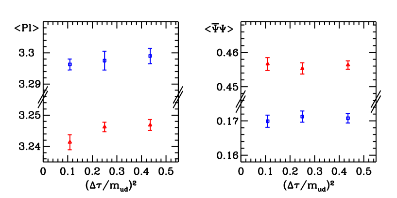
Figure 1: (a) The variation of the plaquette as a function of the step-size squared at $\beta=5.4$ and $m_{q}a=0.064$. The boxes come from the cold and the triangles from the hot lattices. The cold system has a stronger step-size dependence. As it can be seen step-sizes smaller than $m_{ud}/2$ result in smaller systematic uncertainties than the statistical error. (b) The same for the chiral condensate of the light quarks. Their step-size dependence is negligible.

Our simulations employ the standard R-algorithm [38]. The length of one trajectory is unity. The step-size dependence of different relevant quantities (expectation values of the plaquette $\langle Pl\rangle$, or chiral condensate $\langle{\bar{\Psi}}\Psi\rangle$) was already analysed in the literature (see e.g. [39, 31]). We also studied the systematic uncertainties associated with the step-size dependence of the results. Similarly to other groups we found that these effects are much more pronounced for cold lattices. The most sensitive quantity is the plaquette difference between hot and cold lattices. This difference can be of the order of the step-size error. Figure 1 shows the plaquette and the chiral condensate of the light quarks as a function of the step-size squared, which is the leading error in the R-algorithm [38]. Based on these experiences the step-size is chosen to be $m_{ud}/2$. The errors that are introduced this way are 0.2 % for zero temperature lattices and 0.1 % for finite temperature ones.

Statistical uncertainities are determined by jackknife analysis with 20-50 jackknife samples.

Since we usually move along the line of constant physics by changing the lattice spacing $a$ and keeping the masses fixed we will explicitely write out the lattice spacing $a$ in our formulas. In this paper we study lattices with isotropic couplings. In this case the lattice spacing is the same in the temporal and spatial directions. We write $\mu_{B}$ for the baryonic chemical potential, whereas for the quark chemical potential ($u,d$ quarks) we use the notation $\mu$. Similarly, the baryon density is denoted by $n_{B}$ and the light quark density by $n$.

3 Lines of constant physics (LCP) at $\mu=0$

In this section we discuss the role of LCP when determining the EoS in pure gauge theory and in dynamical QCD. After that we determine the lines of constant physics, along which our simulations are done.

The EoS has been determined for pure gauge (quenched) theory on the lattice already in the early years of lattice QCD. Continuum extrapolations have been made by using several lattice actions. The results are in agreement within errorbars [40, 41, 42]. Results obtained by the integral method and the derivative method were also compared [43, 44].

In order to detetermine the temperature $T=1/[N_{t}a(\beta)]$ of the pure gauge theory, we have to compute the lattice spacing ($a$) as a function of the gauge coupling ($\beta$). Note that when changing the coupling of the pure gauge system one automatically remains (upto scaling violations) on the line of constant physics. The situation is quite different in full QCD. In the $d$ dimensional space of the bare parameters one defines $d$ appropriately chosen quantities. The LCP is given by $d-1$ constraints and it is parametrized by a non-constrained combination of the above quantities. For the $2+1$ flavour staggered action we have three bare parameters ($\beta$, and two masses, $m_{ud},m_{s}$). Thus, we need two constraints. There are several possibilities for these constraints and consequently there are many ways to define an LCP. A convenient choice for two of the three quantities can be the bare quark masses ($m_{ud}$ and $m_{s}$). A more physical possibility is to use the pion and kaon masses ($m_{\pi},m_{K}$). There are several options for the third quantity. It can be the rho mass ($m_{\rho}$), the string tension ($\sqrt{\sigma}$), the $R_{0},R_{1}$ scales of the potential ([45], and also [46]) or the transition temperature. Fixing the ratios of the third quantitiy to the first two gives two constraints and the third quantity in lattice units fixes the scale along the LCP.

In our analysis first we use the bare quark masses ($m_{ud}$ and $m_{s}$) and the transition temperature to define an LCP. In this paper we use two LCP’s (LCP₁ and LCP₂). The conditions

$$\begin{array}[]{c}m_{ud}=0.48T_{c}=0.48/(N_{t}a)\ \ \ \ {\rm and}\ \ \ \ \ m_{s}=2.08\cdot m_{ud}\\ m_{ud}=0.384T_{c}=0.384/(N_{t}a)\ \ \ \ {\rm and}\ \ \ \ \ m_{s}=2.08\cdot m_{ud}\end{array}$$ (3)

are used as the constraints for LCP₁ and LCP₂, respectively. For both LCP’s we determined four different transition couplings ($\beta_{c}$) by susceptibility peaks on $N_{t}=1/(T_{c}a)=4$, 6, 8 and 10 lattices with spatial extensions $N_{s}\mathop{\raise 1.29167pt\hbox{$>$\kern-7.5pt\raise-4.73611pt\hbox{$\sim$}}}3N_{t}/2$ and quark masses given by eq. (3). The quark masses or the transition gauge couplings can be used to parametrize the LCP’s.

Note that $m_{s}/m_{ud}$ is the same for both of our LCP’s. This relationship does not change when we interpolate between the two LCP’s or perform reweighting in some parameters. Thus, for transparency we usually do not specify the quark flavours when discussing the physical scale. We simply speak about “quark mass parameter” or “quark mass”. The flavour dependence is indicated explicitely only when necessary.

It is instructive to define LCP’s by using renormalized quantities (LCP^∗’s, namely LCP${}_{1}^{*}$ and LCP${}_{2}^{*}$) and to test scaling violation. One can calculate $m_{\rho},m_{\pi}$, $R_{0}$ and $\sigma$ on $T=0$ lattices ($V=14^{3}\cdot 24$) using the bare parameters obtained for LCP₁ and LCP₂. By measuring these quantities at somewhat different quark masses gives the possibility to define by linear interpolations the LCP^∗’s. Our results for LCP₂ and LCP${}_{2}^{*}$ are summarized in Table 1 and Table 2. The definition of LCP${}_{2}^{*}$ was $m_{\pi}/m_{\rho}\approx 0.626$. As it can be seen different definitions of the scales deviate from each other only by $\approx$ 8 %. Table 1 and Table 2 contains the $T=0$ results for the “non-LCP approach”, too (see next section).

$N_{t}$	$\beta$	$ma$	$\sqrt{\sigma}a$	$R_{0}/a$	$R_{1}/a$	$m_{\rho}a$	$m_{\pi}a$
4	5.271	0.096	0.5889(9)	2.02(1)	1.483(2)	1.421(1)	0.78514(6)
6	5.4	0.064	0.3686(6)	3.19(5)	2.34(2)	1.048(1)	0.6805(1)
8	5.5	0.048	0.2697(5)	3.96(9)	3.64(10)	0.778(4)	0.5595(13)
10	5.58	0.0384	0.2358(4)	4.44(5)	3.71(5)	0.637(4)	0.480(3)
4	5.271	0.1412	0.350(1)	2.94(4)	2.71(3)	1.511(7)	0.9282(3)
6	5.4	0.067	0.426(2)	2.92(7)	2.21(9)	1.076(3)	0.693(10)
8	5.5	0.043	0.344(2)	3.27(28)	2.50(8)	0.933(15)	0.566(1)
10	5.58	0.0304	0.347(2)	2.95(4)	2.72(3)	0.86(3)	0.469(2)
3.2	5.19	0.096	0.6846(11)	1.748(3)	1.327(2)	1.450(5)	0.7677(6)
4	5.27	0.096	0.5899(9)	2.02(1)	1.483(2)	1.421(1)	0.78514(6)
4.8	5.36	0.096	0.4613(6)	2.55(13)	1.81(1)	1.314(3)	0.8045(3)
6.21	5.5	0.096	0.3239(30)	3.85(7)	2.63(1)	1.081(1)	0.803(1)
7	5.58	0.096	0.2716(10)	4.8(1)	2.94(9)	0.9513(8)	0.777(2)

Table 1: Different quantities along LCP₂ (upper part) and the “non-LCP approach” (lower part). The middle part shows new simulation points that were used to determine LCP${}_{2}^{*}$. As usual, the numbers in the parenthesis indicate the estimated statistical errors of the last digits. The effective $N_{t}$ values for the “non-LCP approach” were calculated as follows. We determined four different critical couplings on $N_{t}$=4,6,8 and 10 lattices, while the quark mass was fixed at $ma$=0.096. Effective $N_{t}$-s were determined by interpolating between and slightly extrapolating from these points.

$N_{t}$	$\beta$	$ma$	$\sqrt{\sigma}R_{0}$	$m_{\rho}R_{0}$	$\sqrt{\sigma}R_{1}$	$m_{\pi}/m_{\rho}$
4	5.271	0.096	1.190(8)	2.87(2)	0.874(3)	0.552(4)
6	5.4	0.064	1.176(2)	3.34(6)	0.860(9)	0.649(1)
8	5.5	0.048	1.06(3)	3.08(9)	0.98(3)	0.719(5)
10	5.58	0.0384	1.05(1)	2.83(5)	0.87(1)	0.75(1)
4	5.271	0.1412	1.03(2)	4.44(8)	0.95(1)	0.614(4)
6	5.4	0.067	1.24(4)	3.14(8)	0.94(4)	0.644(11)
8	5.5	0.043	1.12(10)	3.05(31)	0.86(3)	0.60(1)
10	5.58	0.0304	1.02(2)	2.52(12)	0.94(2)	0.55(2)
3.2	5.19	0.096	1.197(3)	2.53(1)	0.908(3)	0.529(3)
4	5.271	0.096	1.190(8)	2.87(2)	0.874(3)	0.552(4)
4.8	5.36	0.096	1.18(6)	3.35(18)	0.835(6)	0.612(3)
6.21	5.5	0.096	1.25(3)	4.16(8)	0.852(11)	0.743(2)
7	5.58	0.096	1.30(3)	4.57(10)	0.80(3)	0.817(3)

Table 2: Dimensionless combinations along LCP₂ (upper part) and the “non-LCP approach” (lower part). The middle part shows new simulation points that were used to determine LCP${}_{2}^{*}$. Quark mass dependent dimensionless quantities change more in the “non-LCP approach”.

By the finite temperature technique, described above, only a few points of the LCP’s can be obtained. To interpolate $\beta(a)$ between these points (and extrapolate slightly away from them) we use the renormalization group inspired ansatz proposed by Allton [47]. Note that not only the quark mass parameter ($m_{q}a$) can be used as a parameter of the LCP’s, but a particularly illustrative parametrization is obtained by inverting eq. (3) and using $N_{t}$ as a continuous parameter. (We use later this $N_{t}$ parametrization for constructing the LCP on the $\mu-\beta$ plane by a linear combination of LCP₁ and LCP₂, see Section 5.) Figure 2 shows LCP₁ and LCP₂ with our simulation points. A line of constant physics obtained by renormalized quantities (LCP${}_{2}^{*}$) and the simulation points in the “non-LCP” approach are also shown. Note that even though the determination of the LCP₁ and LCP₂ are done on finite temperature lattices, the obtained bare parameters are used in the rest of the paper for $T=0$ and $T\neq 0$ simulations.

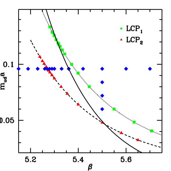
Figure 2: The lines of constant physics (LCP₁ and LCP₂) on the $\beta$ vs. $m_{ud}a$ plane. The strange quark mass is given by $m_{s}=2.08m_{ud}$ for both LCP’s. The simulation points are shown by squares/triangles and connected by dashed/dotted lines for LCP₁/LCP₂, respectively. An approximate LCP obtained by renormalized quantities (LCP${}_{2}^{*}$, the definition is $m_{\pi}/m_{\rho}\approx 0.626$) is shown by a solid line. The diamonds along a horizontal line represent the simulation points in the “non-LCP” approach. Additional 3 diamonds in the vertical direction show the simulation points used to test the path independence of the integral method (see next Section).

4 Equation of state along the lines of constant physics (LCP) at $\mu=0$

In previous studies of the EoS with staggered quark actions, the pressure and the energy density were determined as functions of the temperature for fixed value of the bare quark mass $m_{q}a$ in the lattice action [31, 32, 33]. In these studies a fixed $N_{t}$ was used (e.g. $N_{t}=4$ or 6) at different temperatures. Since $T=1/(N_{t}a)$ the temperature is set by the lattice spacing which changes with $\beta$. This convenient, fixed bare $m_{q}a$ choice leads to a system which has larger and larger physical quark masses at decreasing lattice spacings (thus, at increasing temperatures). Increasing physical quark masses with increasing temperatures could result in systematic errors of the EoS.

Clearly, instead of this sort of analysis (in the rest of the paper we refer to it as “non-LCP approach”) one intends to study the temperature dependence of a system with fixed physical observables, therefore on an LCP.

Recently, the EoS was also studied by using an action with dynamical Wilson quarks [48]. In this case there is no convenient choice similar to the approach with fixed $m_{q}a$ (“non-LCP approach”). The authors determined the lines of constant physics and the $\beta$ functions. They obtained the EoS along different LCP’s in the range of $m_{\pi}/m_{\rho}=0.65-0.95$.

In our analysis we use full QCD with staggered quarks along the LCP and compare these results with those of the “non-LCP approach”.

In order to be self-contained in this Section we review the $\mu=0$ technique to determine the interaction measure ($\epsilon-3p$) by using the non-perturbative $\beta$-function. Then we shortly discuss the integral method [34] to determine the pressure. In practice, the energy density, entropy density or the speed of sound can be directly deduced from the interaction measure and the pressure (c.f. $sT=\epsilon+p$ and $c_{s}^{2}=dp/d\epsilon$). We review the basic formulas and emphasize the issues related to the EoS determination along an LCP.

The energy density and pressure are defined in terms of the free-energy density ($f$):

$$\epsilon(T)=f-T\frac{\partial{f}}{\partial{T}},\ \ \ \ \ \ \ \ p(T)=-f.$$ (4)

Expressing the free energy in terms of the partition function ($f=-T/V\log Z=$
$-T\partial(\log Z)/\partial V$) we have:

$$\epsilon(T)=\frac{T^{2}}{V}\frac{\partial{\log Z}}{\partial{T}},\ \ \ \ \ \ \ \ p(T)=T\frac{\partial(\log Z)}{\partial V}.$$ (5)

As mentioned before, we use the same lattice spacings in the temporal and spatial directions. The temperature and volume are connected to this lattice spacing by

$$T=\frac{1}{aN_{t}}, V=a^{3}N_{s}^{3}.$$ (6)

By varying the bare parameters one can change the lattice spacing; however, it is not possible to change $T$ and $V$ independently. This is the reason why eqs. (5,6) cannot be used directly. Instead one determines the interaction measure by the help of the $\beta$ function and the pressure by using the integral method.

Inspecting eqs.(5, 6) we see that the interaction measure $(\epsilon-3p)/T^{4}$ is directly proportional the total derivative of $\log Z$ with respect to the lattice spacing:

$$\frac{\epsilon-3p}{T^{4}}=-\frac{N_{t}^{3}}{N_{s}^{3}}a\frac{d(\log Z)}{da}.$$ (7)

Here, the derivative with respect to $a$ is defined along the LCP, which means that only the lattice spacing changes and the physics (in our case $m_{q}/T_{c}$) remains the same. The variation of the lattice spacing can be controlled by the bare parameters of the action ($\beta$ and $m_{q}a$), so we can write:

$$\frac{d}{da}=\frac{\partial\beta}{\partial a}\frac{\partial}{\partial\beta}+\sum_{q}\frac{\partial(m_{q}a)}{\partial a}\frac{\partial}{\partial(m_{q}a)}.$$ (8)

The partial derivatives with respect to $a$ should be taken along the LCP. Since the LCP is defined by $m_{q}/T_{c}={\rm const.}$, the partial derivative $\partial(m_{q}a)/\partial a$ becomes simply $m_{q}$. The derivatives of $\log Z$ with respect to $\beta$ and $m_{q}$ are the plaquette and $\bar{\Psi}\Psi_{q}$ averages multiplied by the lattice volume. We get:

$$\frac{\epsilon-3p}{T^{4}}=-N_{t}^{4}a\left(\overline{{\rm Pl}}\left.\frac{\partial\beta}{\partial a}\right|_{\rm LCP}+\sum_{q}\overline{\bar{\Psi}\Psi}_{q}m_{q}\right).$$ (9)

The pressure is the other basic quantity, which is usually determined by the integral method [34]. The pressure is simply proportional to $\log Z$, however it cannot be measured directly. One can determine its partial derivatives with respect to the bare parameters. Thus, we can write:

$$\frac{p}{T^{4}}=\left[-\frac{N_{t}^{3}}{N_{s}^{3}}\int^{(\beta,m_{q}a)}_{(\beta_{0},m_{q0}a)}d(\beta,m_{q}a)\left(\begin{array}[]{c}{\partial\log Z}/{\partial\beta}\\ {\partial\log Z}/{\partial(m_{q}a)}\end{array}\right)\right]-\frac{p_{0}}{T^{4}}.$$ (10)

Since the integrand is the gradient of $\log Z$, the result is by definition independent of the integration path. We need the pressure along the LCP, thus it is convenient to measure the derivatives of $\log Z$ along the LCP and perform the integration over this line. For the subtracted vacuum term we used the zero temperature pressure, i.e. the same integral on $N_{t0}=N_{s}$ lattices. The lower limits of the integrations (indicated by $\beta_{0}$ and $m_{q0}$) were set sufficiently below the transition point. By this choice the pressure becomes independent of the starting point (in other words it vanishes at vanishing temperature). In the case of $2+1$ staggered QCD eq. (10) can be rewritten appropriately and the pressure is given by

$$\frac{p}{T^{4}}=-N_{t}^{4}\int^{(\beta,m_{q}a)}_{(\beta_{0},m_{q0}a)}d(\beta,m_{ud}a,m_{s}a)\left(\begin{array}[]{c}\langle{\rm Pl}\rangle\\ \langle\bar{\Psi}\Psi_{ud}\rangle\\ \langle\bar{\Psi}\Psi_{s}\rangle\end{array}\right),$$ (11)

where we use the following notation for subtracting the vacuum term:

$$\langle{\cal O}(\beta,m)\rangle={\overline{{\cal{O}}}(\beta,m)}_{T\neq 0}-{\overline{{\cal O}}(\beta,m)}_{T=0}.$$ (12)

The integral method was originally introduced for the pure gauge case for which the integral is one dimensional, it is performed along the $\beta$ axis. Previous studies for staggered dynamical QCD [31, 32, 33] used a one-dimensional parameter space. Note that for full QCD the integration should be performed along a path in a multi-dimensional parameter space. In our $2+1$ flavour staggered QCD case the parameter space is three-dimensional.

According to eq.(10) the gradient of $\log Z$ is measured, thus the integral should be independent of the path. We explicitely checked this independence by performing the integration along different paths. For this purpose we determined the normalised pressure ($p/T^{4}$) at $\beta=5.5$, $m_{ud}=0.048$ (this point corresponds to $T=2T_{c}$ with quark masses defined by eq.(3)). In the calculation two different integration paths were used. In the first case we integrated along the LCP. We obtained $p/T^{4}=6.15(5)$. In the second case the integration path contained two pieces (see the path defined by the diamonds of Figure 2). The first piece is a $\beta$ integral at constant $m_{q}$, the second one is a $m_{ud},m_{s}$ integral (with fixed mass ratio) at constant $\beta$ value. For the second path we obtained $p/T^{4}=6.15(4)$. As it can be seen the two different paths give the same result for the pressure (within the estimated uncertainties).

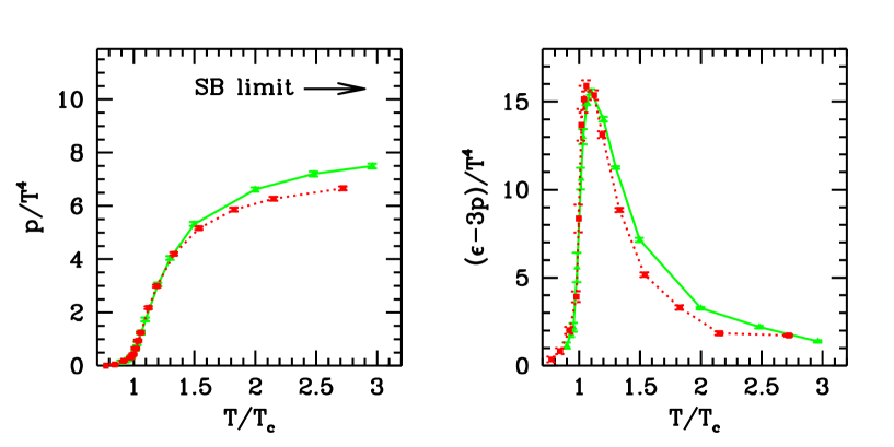
Figure 3: The equation of state at $\mu$=0. (a) The left panel shows the pressure $p$, as a function of the temperature. All quantities are normalised by $T^{4}$. The solid line connects the data points obtained along the LCP₂, whereas the dashed line connects the data points obtained in the “non-LCP approach” (see text). The Stefan-Boltzmann limit is also shown by an arrow for $N_{t}$=4 lattices. The EoS along the LCP and the “non-LCP approach” differ from each other at high $T$. (b) The same for the “interaction measure” ($\epsilon$-3p).

The EoS is determined along the LCP’s and also by using the “non-LCP approach”. The results along LCP₂ and LCP₁ are very close to each other (the $T=0$ pion masses differ only by 10% for the two LCP’s; for the $m_{\pi}/m_{\rho}$ dependence of the EoS with Wilson quarks see [48]). Figure 3 shows the EoS at vanishing chemical potential on $N_{t}=4$ lattices for LCP₂ and for the non-LCP approach. The pressure and $\epsilon-3p$ are presented as a function of the temperature. The parameters of LCP₂ and those of the non-LCP approaches coincide at $T=T_{c}$. The Stefan-Boltzmann limit valid for $N_{t}=4$ lattices is also shown.

It is interesting to compare the pressure difference between LCP and non-LCP approaches at finite temperature in case of the ideal and interacting gas. In the ideal gas case there is a relative 2.7% difference between the pressures, while this difference is three times larger in the interacting case (9.4%) at $T=2.5\cdot T_{c}$. This means that considering only the mass-effect of the ideal gas, we would make a significant underestimation for the interacting case.

5 Reliability of reweighting

In order to determine the EoS for the $\mu\neq 0$ case (when direct simulations are not possible) we use the multi-parameter reweighting proposed in [17] The aim of this section is to point out that the multi-parameter reweighting [17] is reliable. (For another study of reweighting see [49].) We also determine its region of validity by a suitably estimated error. Furthermore we show that in certain cases the multi-parameter reweighting is much more reliable than single-parameter techniques (Glasgow-type reweighting [18]) in the sense that one can reach farther regions. On top of this we demonstrate that the major requirement to be met by the sample used for the reweighting is that it should be as variable as possible. Variability here means that it should contain configurations from the various phases or configurations from the different Z(3) sectors in case of imaginary chemical potentials. To start with let us briefly review the multi-parameter reweighting.

As proposed in [17] one can identically rewrite the partition function in the form:

$$Z(m,\mu,\beta)=\int{\cal D}U\exp[-S_{bos}(\beta_{0},U)]\det M(m_{0},\mu=0,U)$$ (13)

$$\left\{\exp[-S_{bos}(\beta,U)+S_{bos}(\beta_{0},U)]\frac{\det M(m,\mu,U)}{\det M(m_{0},\mu=0,U)}\right\},$$

where $U$ denotes the gauge field links and $M$ is the fermion matrix . The chemical potential $\mu$ is included as $\exp(a\mu)$ and $\exp(-a\mu)$ multiplicative factors of the forward and backward timelike links, respectively. In this approach we treat the terms in the curly bracket as an observable – which is measured on each independent configuration, and can be interpreted as a weight – and the rest as the measure. Thus the simulation can be performed at $\mu=0$ and at some $\beta_{0}$ and $m_{0}$ values (Monte-Carlo parameter set). By using the reweighting formula (13) one obtains the partition function at another set of parameters, thus at $\mu\neq 0$, $\beta\neq\beta_{0}$ or even at $m\neq m_{0}$ (target parameter set).

Expectation values of observables can be determined by the above technique. In terms of the weights (i.e. the expression in the curly bracket of eq. (13)) the averages can be determined as:

$${\overline{\cal O}}(\beta,\mu,m)=\frac{\sum\{w(\beta,\mu,m,U)\}{\cal O}(\beta,\mu,m,U)}{\sum\{w(\beta,\mu,m,U)\}}.$$ (14)

It is clear that simulating at a given Monte Carlo parameter set the errors increase as we go farther and farther with the target parameter set. We need an error estimate of the reweighted quantities which shows how far we can reweight in the target parameter space. This way we could determine the borderline of the region outside of which the reweighting already fails to give reliable predictions. To achieve this we checked several error definitions including the jackknife and the statistical errors described in the papers [50, 51]. Both proved little to draw the limit of the reweighting procedure. The reason for this is that neither of them contains the systematic errors occuring because of the finite sample size. We note that in [51] there is an error estimate recommended for taking the finite sample size into consideration. However, this estimate uses an approximation of the distribution of the sample. An approximation of this kind can not be justified in case of staggered dynamical QCD.

Eventually, with a new technique different from the ones mentioned above we succeeded to define a reliable error estimate for the reweighted quantities and to draw the limit of the reweighting procedure. After defining the new technique we show its application on an example. Then we demonstrate the problems that crop up while using the jackknife error and furthermore show how our new method overcomes these difficulties.

The steps of the new procedure are as follows. First we assign to each and every starting configuration the weight $w$ valid at the chosen target parameter set i.e.

$$w=\exp\left\{\Delta\beta\cdot V\cdot(Pl)+\frac{n_{f}}{4}[\ln\det M(\mu)-\ln\det M(\mu=0)]\right\}$$ (15)

where $V$ is the lattice volume. Note that only the $\beta$ and the $\mu$ parameters differ from their values at the simulation point. We generate a new set of configurations using these weights for Metropolis-like accept-reject steps. Let the original and new configuartions be $\Phi_{i}$ and $\Phi^{\prime}_{i}$ and the corresponding weights (according to eq. (15)) $w_{i}$ and $w^{\prime}_{i}$. The first new configuration is $\Phi^{\prime}_{1}=\Phi_{1}$. Then for $i>1$, $\Phi^{\prime}_{i}=\Phi_{i}$ with the probability ${\rm max}\{1,\frac{w_{i}}{w^{\prime}_{i-1}}\}$ and $\Phi^{\prime}_{i}=\Phi^{\prime}_{i-1}$ otherwise. For complex weights we have to take either the absolute values or the absolute values of the real parts of the weights. The $\Phi^{\prime}_{i}$ configurations of the new sample are taken with a unit weight to calculate expectation values, variances and integrated autocorrelation times [50] (the latter grows at every rejection due to the repetition of certain configurations). If our initial sample consisted of a large number of independent configurations then for real weights this method regenerates a sample which is theoretically perfect for the target parameters. For complex weights the new set of configurations can not be used to measure observables, but it can be used for getting an error estimate. Therefore, in general, we will use eq. (14) to get the expectation values and the newly generated sample to determine the errors (see later).

We still have to clarify two important points before our new procedure is finalised. The first is the question of thermalization. The second question is (in an extreme case): what happens if there is no configuration in the starting sample which would be relevant at the target parameters. We solved the first problem by defining a thermalization segment at the beginning of every newly generated sample which we cut off from the sample before calculating the expectation values and the errors. An obvious assumption is to claim that the already thermalized sample containing valuable information starts with the first different configuration right after the one with the largest weight. This ensures that if there is only one configuration in the initial sample which “counts” at the target parameters then this information will not be lost. The second problem can not be solved perfectly. The problem occurs e.g. when a phase transition is very strong, that is the physical quantities change significantly during the transition (first order transition) and we would like to reweight starting from deep inside in one phase into deep inside into the other phase. Then the solution can only be a huge sample size (or small lattice size) which allows the presence of a few configurations of the target phase in the initial sample. It is, however, difficult to define what a huge sample really means in a general, practical way.

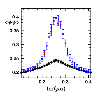
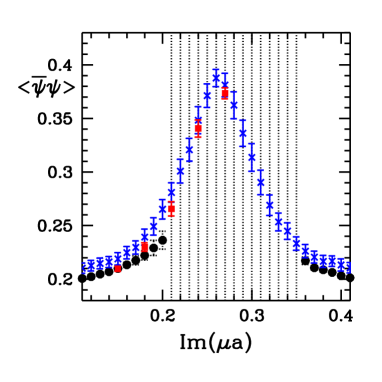
Figure 4: (a) The left panel shows $\bar{\psi}\psi$ expectation values and error estimates of three different methods. The squares correspond to direct simulations (out of $60000$ configurations). The crosses denote the results of the multi-parameter reweighting method (out of $\approx 1200$ independent configurations) while the circles are the points of the Glasgow-type reweighting (out of $\approx 1200$ independent configurations). In case of the latter two methods the error estimates are determined using the new Metropolis-type method. (b) In the right panel the meaning of the symbols are unchanged but the sample sizes for the reweighting techniques are increased to 2500 independent configurations in case of the multi-parameter reweighting and to 7000 in case of the Glasgow-type reweighting. In case of the multi-parameter reweighting the increased sample size only decreases the error estimate, maintaining consistency with the direct simulation result. On the other hand in case of the Glasgow-type reweighting the fact that the small sample (used in the left panel) does not contain any configuration from the target phase causes systematic errors in the expectation values and mainly in their uncertainties. This is because in case of strong phase transitions – like in our case – it is far too difficult to define a reliable thermalization stage by virtue of the weights. Increasing the sample size helps in this situation leading to the results of the right panel. The very large error estimates in the Glasgow case are realistic, the prediction does agree within errors with the direct simulation result.

To illustrate the new technique let us take a look at the $n_{f}=4$ flavour case at $m_{q}a=0.05$ bare quark mass on $4\cdot 6^{3}$ size lattice at imaginary chemical potential. Note that for purely imaginary chemical potentials direct simulation is possible, therefore it is possible to check the validity of any error estimation method. Direct simulation is thus used as a standard. Accordingly, we determine the plaquette ($Pl$) and the $\bar{\psi}\psi$ expectation values and their uncertainties at $\beta=5.085$ and Im$(\mu)\neq 0$, that is at the target, imaginary chemical potential values using three different techniques. First technique is direct simulation (60000 configurations). The other two methods are based on reweighting Im$(\mu)=0$ data. We carried out simulations at Im$(\mu)=0$ in the phase transition point, i.e. at $\beta=5.04$ ($\approx 2500$ independent configurations) and at $\beta=5.085$ ($\approx 7000$ independent configurations). From these two starting points with the use of the reweighting we predicted the plaquette ($Pl$) and the $\bar{\psi}\psi$ expectation values and their uncertainties at $\beta=5.085$ and Im$(\mu)\neq 0$, that is at the target. In the following we refer to the technique starting from the phase transition point at Im$(\mu)=0$ as multi-parameter reweighting, while the technique starting from $\beta=5.085$ (fixed at the target value) and Im$(\mu)=0$ as Glasgow-type reweighting. We used the new Metropolis-type method defined above in both cases. As a check for both starting points we also calculated the plaquette and the $\bar{\psi}\psi$ expectation values directly by (14) at the target points, and observed that the results are very similar to the results obtained by the Metropolis-type method.

The expectation values and their errors obtained by the new (Metropolis-type) method along with the direct simulation points are shown on the left panel of Figure 4. When making the figure we had to make use of an additional information, namely the fact that the $\beta-$Im$(\mu)$ plane consists of three sectors. If we want to make predictions about all of them based on the data at $\mu=0$ we can do it by explicitely using the Z(3) symmetry. That is we use the starting sample in such a way that every plaquette value is included three times: once with the original weight and also with the weights of shifted to $\mu\pm i\pi/N_{t}/3$ $\mu$ arguments. Performing the reweighting like this we obtained Figure 4. In the left panel the second problem mentioned in the previous paragraph is seen. I.e. in case of Glasgow-type reweighting the small sample (1200 independent configurations) causes the problem. Namely, it does not contain any configuration belonging to the target phase when the target chemical potential is around Im($\mu)=\pi/12$. Then even our new method gives misleading results. Increasing the samples size, as soon as a single, dominant configuration turns up, the new method supplies us with reliable error estimates. (See the right panel of Figure 4, where we used 7000 independent configurations in place of the 1200 configurations that lead to the wrong results on the left panel.) The right panel truly reflects the correctness of the multi-parameter reweighting in contrast to the single-parameter reweighting Glasgow- method. The infinitely large errors of the Glasgow-method indicate that the whole sample is thermalization, that is it does not provide information about the expectation value in the corresponding imaginary chemical potential points.

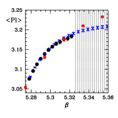
Figure 5: Plaquette expectation values obtained by direct simulations and reweighting at various $\beta$-s. The squares and their errorbars denote the results of direct simulation. The initial sample used for reweighting consisted of 33000 configurations. The parameters were: $\beta=5.274$, the critical $\beta$ in the $n_{f}=2+1$ flavour case when $m_{u,d}=0.096$, $m_{s}=2.08m_{u,d}$ are the quark masses (in lattice units) on a $4\cdot 8^{3}$ size lattice. The circles and the errorbars belonging to them represent the newly introduced Metropolis-type method. Infinitely large errors mean that the whole, newly generated sample is thermalization so it does not contain information about the distribution at the $\beta$ parameter in question. The crosses refer to the values given by the formula (5.2), the errors assigned to them are jackknife errors. It is clear that the jackknife errors do not notice the limit of validity of the reweighting procedure, but for small $|\Delta\beta|$-s they provide a good error estimate.

An example of the troubles occuring when using the jackknife error estimate will be shown in case of single-parameter reweighting in the $\beta$ parameter. Thus one can use the new (expensive) error estimate to provide the limit of the applicability of the reweighting procedure after which the simpler jackknife method can be applied in the appropriate region. (This strategy was followed in the rest of the paper to calculate the EoS.) In our example we take $4\cdot 8^{3}$ size lattice in case of $m_{u,d}=0.096$, $m_{s}=2.08m_{u,d}$ bare quark masses (in lattice units) at the critical point, i.e. at $\beta=5.274$. A sample simulated in this point consisting of 33000 configurations was reweighted by (14). We evaluated the errors of the reweighted quantities by the Metropolis-type and by the jackknife methods. These are shown together with the reweighted plaquette expectation values in Figure 5. It can be seen that the new method gives information on the errors and also on the limit of the applicability of the reweighting procedure. On the other hand the jackknife error can not be used outside a restricted region and does not provide any clue on the region of applicability of the reweighting procedure.

What can we say about the errors in the real $\mu$ case based on the new error estimation procedure? The Metropolis steps can only be taken using either the absolute values or the absolute values of the real parts of the weights. It is clear that both possibilities represent only approximations to the true reweighting given by eq. (14). Whereas the expectation values provided by equation (14) are exact in principle, we may test the above defined Metropolis-type procedures for the errors provided by them. We can claim based on Figure 6 that on a $4\cdot 8^{3}$ size lattice in the $\mu\in[0,0.3]$ region and also in all other examined cases the three methods do not provide significantly different expectation values, differences are tolerated in the errors. So we assign the errors of the Metropolis-type method given through the use of the absolute values of the real parts of the weights to the expectation values obtained from equation (14).

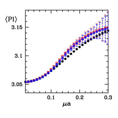
Figure 6: Average plaquette versus the real chemical potential. 33000 configurations were simulated at the parameter set: $\beta=5.274$, $m_{u,d}=0.096$, $m_{s}=2.08m_{u,d}$ on a $4\cdot 8^{3}$ size lattice. This is at the critical $\beta$ in the $n_{f}=2+1$ flavour case. The circles refer to the plaquette values given by (5.2), their errorbars indicate jackknife errors. The squares belong to a Metropolis-type method using the absolute values of the real part of the weights while in case of the triangles the absolute values of the weights were used. In both cases the errors are given by the square roots of the variances times the autocorrelation time.

6 Best reweighting lines and the LCP’s

We can define reweighting lines on the $\beta$–$\mu$ plane so as to make the least possible mistake during the reweighting procedure. To do this we introduce the notion of overlap measure which we denote by $\alpha$. The overlap measure is the normalised number of different configurations in the sample created with the Metropolis-type reweighting after cutting off the thermalization. We plotted the contour lines of $\alpha$ in the left panel of Figure 7. The dotted areas are unattainable, that means here the overlaps vanish, the errors are infinitely large. The best reweighting lines can be defined for each simulation point. For a given value of $\mu$ we choose $\beta$ corresponding to the maximal value of $\alpha$. The points of the best reweighting line are given by the rightmost points of the contours of constant overlap in Figure 7 a.

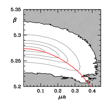
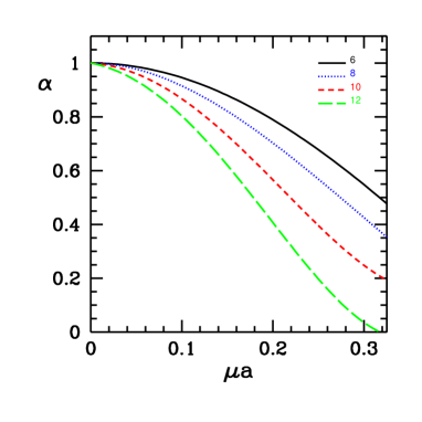
Figure 7: (a) The left panel shows the real chemical potential–$\beta$ plane. 33000 configurations were simulated at the parameter set: $\beta=5.274$, $m_{u,d}=0.096$, $m_{s}=2.08m_{u,d}$ on a $4\cdot 8^{3}$ size lattice. This is at the critical $\beta$ in the $n_{f}=2+1$ flavour case. The dotted lines are the contours of the constant overlap. The dotted area is the unknown territory where the overlap vanishes, i.e. the sample regenerated from the initial one consists of nothing but thermalization. The roughness of the border separating the unknown territory is due to the presence of random numbers in the procedure. The solid line is the phase transition line determined by the peaks of susceptibility. (b) In the right panel the volume and the $\mu$ dependence of the overlap ($\alpha$) is shown. Upper curves correspond to smaller lattice sizes, $4\cdot 6^{3}$, $4\cdot 8^{3}$, $4\cdot 10^{3}$ and $4\cdot 12^{3}$ respectively. The half width ($\mu_{1/2}$; defined by $\alpha\left.\right|_{\mu_{1/2}}=1/2$) scales according to: $\mu_{1/2}\propto V^{-\gamma}$ with $\gamma\approx 1/3$.

It is important to examine the volume dependence of reweighting by using the notion of the overlap. The right panel of Figure 7 shows the $\mu$ dependence of the overlap at fixed $\beta$ and quark mass parameters for different volumes ($V=4\cdot 6^{3}$, $4\cdot 8^{3}$, $4\cdot 10^{3}$ and $4\cdot 12^{3}$). As expected, for fixed $\mu$ larger volumes result in worse overlap. One can define the “half-width” ($\mu_{1/2}$) of the $\mu$ dependence by the chemical potential value at which $\alpha=1/2$. One observes an approximate scaling behaviour for the half-width: $\mu_{1/2}\propto V^{-\gamma}$ with $\gamma\approx 1/3$, which is much better than a crude $1/\sqrt{V}$ estimate. Thus the volume dependence of $\mu-\beta$ reweighting is less restrictive than that of reweightings in other parameters.

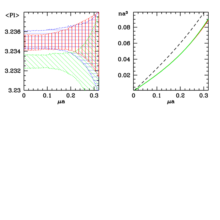
Figure 8: (a) The $\mu$ dependence of the plaquette (left panel). Results obtained on $4\cdot 8^{3}$ lattices are shown by horizontally, those on $4\cdot 10^{3}$ lattices are shown by vertically and those on $4\cdot 12^{3}$ are shown by diagonally lined bands. The results agree within their statistical errors. (b) The $\mu$ dependence of fermion number density (right panel). The difference of $4\cdot 8^{3}$, $4\cdot 10^{3}$ and $4\cdot 12^{3}$ results cannot be resolved (solid line). The dashed line shows the Stefan-Boltzman limit. Simulations were done at $\beta=5.35$.

Expectation values of observables at finite chemical potential are determined according to eq. (14). There are quantities (e.g. plaquette, Wilson-loop, Polyakov-line) for which the $\mu$ reweighting means only a change in the weight of the configuration but not in the value of the observable. For other quantites (e.g. chiral condensate, fermion number) not only the weight but also the value is influenced by the chemical potential since they are directly expressed by the fermion matrix. It is instructive to study the volume dependence of both types of these quantities. The left panel of Figure 8 shows the average plaquette, the right panel the fermion number density, as functions of the chemical potential. Both quantites are determined on $4\cdot 8^{3}$, $4\cdot 10^{3}$ and $4\cdot 12^{3}$ lattices. The volume dependence is practically negligible for the fermion number density, whereas it is moderate for the average plaquette.

It is obvious that the two-parameter reweighting used in the previous section does not follow the LCP ($\beta$ gets smaller but the quark mass remains $m_{0}a$). We show in the following that the best reweighting line along the LCP can be practically determined by two techniques: a. three-parameter reweighting, b. interpolating method.

a. As it can be seen in the left panel of Figure 7, the change in $\beta$ is not very large for the two-parameter reweighting. Therefore, one can remain on the LCP by a simultaneous, small change of the mass parameter of the lattice action. This results in a three-parameter reweighting (reweighting in $ma$, $\beta$ and $\mu a$). For some fixed $\mu_{target}$ two constraints are needed to determine $m_{target}a$ and $\beta_{target}$. One of them is the generalization of the new, Metropolis-type reweighting to some $m_{target}a\neq m_{0}a$ and the other one is the LCP, which relates the mass parameter to the gauge coupling, i.e. one has to fulfill the following condition

$$\beta_{target}=\beta_{LCP}(m_{target}a).$$ (16)

Similarly to the two-parameter reweighting one can construct the best three-parameter reweighting line, which is shown in Figure 9.

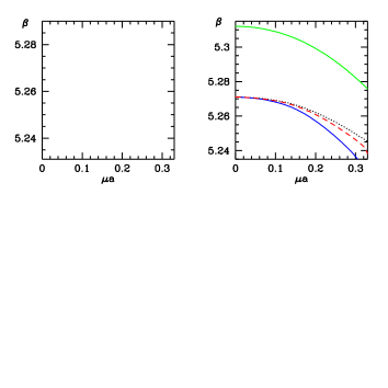
Figure 9: Different types of best weight lines are shown on the $\mu$-$\beta$ plane. Three-parameter ($m$, $\beta$ and $\mu$) reweighting is used for the parameter set of LCP${}_{2}(N_{t}=4)$ (dashed line). Along the line the system remains on the LCP, the small change in $\beta$ is compensated by the change of the mass parameter. Two parameter reweighting is used for the parameter set of LCP${}_{1}(N_{t}=4)$ (upper solid line) and for that of LCP${}_{2}(N_{t}=4)$ (lower solid line). The interpolating technique is used to determine the line of constant physics on the $\mu$-$\beta$ plane (dotted line). Note that the results of the three-parameter reweighting technique and that of the interpolating technique agree within the statistical uncertainties.

b. The other possibility to stay on the line of constant physics at finite $\mu$ is the interpolating technique. One uses the two-parameter reweighting for two LCP’s and interpolates between them. As we discussed in Section 3 not only the mass parameter, but also $N_{t}$ (as a continuous parameter) can be used to parametrize the LCP’s. Thus the data of Figure 2 give $\beta_{1}(N_{t},\mu=0)$ for LCP₁ and $\beta_{2}(N_{t},\mu=0)$ for LCP₂, respectively. The same $N_{t}$ values for the two LCP’s correspond to different mass parameters, which can be written as $(am)_{1}=(am)_{1}(\beta_{1},N_{t},\mu=0)$ and $(am)_{2}=(am)_{2}(\beta_{2},N_{t},\mu=0)$. Note that the two-parameter reweighting to finite $\mu$ does not change the mass parameter. Let us take some fixed $N_{t}$ value and perform two-parameter reweightings for both $\beta_{1}$ and $\beta_{2}$ parameter sets. This results in $\beta_{1}(\mu)$ and $\beta_{2}(\mu)$ best weight lines (these functions for $N_{t}$=4 are shown in Figure 9 by solid lines). Though these individual curves leave the LCP-s, there is a way to stay on e.g. LCP₂ by interpolating between $\beta_{1}(\mu)$ and $\beta_{2}(\mu)$. Since the mass parameters of LCP₁ and LCP₂ are close to each other we use a linear interpolation between them. The obtained gauge coupling is $\beta_{i}(\mu)$ and the mass parameter is $(am)_{i}(\mu)$.

$$\beta_{i}(\mu)=\zeta\beta_{1}(\mu)+(1-\zeta)\beta_{2}(\mu),$$ (17)

$$(am)_{i}(\mu)=\zeta(am)_{1}(\beta_{1},N_{t},\mu=0)+(1-\zeta)(am)_{2}(\beta_{2},N_{t},\mu=0),$$

$$\beta_{i}=\beta_{2}((am)_{i}).$$

The first two equations define the interpolation and the third condition guarantees that we stay on LCP₂. These three equations determine the three unknown variables: $\beta_{i}$, $(am)_{i}$ and the interpolating parameter $\zeta$. The best weight line obtained by the interpolation technique is also shown in Figure 9. As it can be seen the result of this method and the predicition of the three-parameter reweighting agree quite well. This indicates that the requirement for the best overlap selects the same weight lines even for rather different methods.

7 Equation of state at non-vanishing chemical potential

In this section we study the EoS at finite chemical potential. Since we are interested in the physics of finite baryon density we use $\mu=\mu_{u}=\mu_{d}\neq 0$ for the two light quarks and $\mu_{s}=0$ for the strange quark. The same technique and the same equations could be used for the $\mu_{s}\neq 0$ case (one should simply add the strange quark contribution to that of the light quarks).

The energy density and pressure can be derived in a similar way as in the case of vanishing chemical potential discussed in Section 4. However, now the grand canonical potential ($\omega$) is used instead of the free energy. The definitions are:

$$\epsilon(T,\mu)=\omega-T\frac{\partial{\omega}}{\partial{T}}-\mu\frac{\partial{\omega}}{\partial{\mu}},\ \ \ \ \ \ \ \ p(T,\mu)=-\omega.\ \ \ \ \ \ \ \ \$$ (18)

Expressing the grand canonical potential in terms of the grand canonical partition function ($\omega=-T/V\log Z_{gc}$) we get similar results as in the $\mu=0$ case. In order to make this transparent we explain the calculation in detail. As usual one has to separate the space-like ($a_{s}$) and time-like ($a_{t}$) lattice parameters. This way the derivatives with respect to $T$, $V$ and $\mu$ can be replaced by derivatives with respect to $a_{s}$, $\xi$, and $\hat{\mu}$, where $\xi=a_{t}/a_{s}$, $\hat{\mu}=\mu a_{s}$. It does not matter whether we write $\mu a_{t}$ or $\mu a_{s}$, because we will set $\xi=1$ at the end of calculation. The new (lattice) variables can be expressed by the old (thermodynamical) ones:

$a_{s}=\frac{1}{N_{s}}V^{1/3},$

$\xi=\frac{N_{s}}{N_{t}}\frac{1}{TV^{1/3}}$,

$\hat{\mu}=\frac{1}{N_{s}}\mu V^{1/3}.$

And the derivatives:

$$\left.\frac{\partial}{\partial T}\right|_{V,\mu} = -\xi^{2}N_{t}a_{s}\left.\frac{\partial}{\partial\xi}\right|_{a_{s},\hat{\mu}},$$

$$\left.\frac{\partial}{\partial V}\right|_{T,\mu} = \frac{1}{3V}\left(a_{s}\left.\frac{\partial}{\partial a_{s}}\right|_{\xi,\hat{\mu}}-\xi\left.\frac{\partial}{\partial\xi}\right|_{a_{s},\hat{\mu}}+\hat{\mu}\left.\frac{\partial}{\partial\hat{\mu}}\right|_{a_{s},\xi}\right)$$

$$\left.\frac{\partial}{\partial\mu}\right|_{T,V} = a_{s}\left.\frac{\partial}{\partial\hat{\mu}}\right|_{a_{s},\xi}.$$

In particular, for $\epsilon-3p$ we have:

$$\epsilon-3p=\frac{T^{2}}{V}\left.\frac{\partial\log Z_{gc}}{\partial T}\right|_{V,\mu}-3T\left.\frac{\partial\log Z_{gc}}{\partial V}\right|_{T,\mu}+\frac{\mu T}{V}\left.\frac{\partial\log Z_{gc}}{\partial\mu}\right|_{V,T}.$$

Now we replace thermodynamical variables to lattice variables

$$\epsilon-3p = -\frac{T}{V}\xi\left.\frac{\partial\log Z_{gc}}{\partial\xi}\right|_{a_{s},\hat{\mu}}+\frac{\mu T}{V}a_{s}\left.\frac{\partial\log Z_{gc}}{\partial\hat{\mu}}\right|_{a_{s},\xi}-$$ (19)

$$\frac{T}{V}\left(a_{s}\left.\frac{\partial\log Z_{gc}}{\partial a_{s}}\right|_{\xi,\hat{\mu}}-\xi\left.\frac{\partial\log Z_{gc}}{\partial\xi}\right|_{a_{s},\hat{\mu}}+\hat{\mu}\left.\frac{\partial\log Z_{gc}}{\partial\hat{\mu}}\right|_{a_{s},\xi}\right)$$

$$= -\frac{T}{V}a_{s}\left.\frac{\partial\log Z_{gc}}{\partial a_{s}}\right|_{\xi,\hat{\mu}}.$$

Setting $\xi=1$ we get:

$$\frac{\epsilon-3p}{T^{4}}=\left.-\frac{N_{t}^{3}}{N_{s}^{3}}a\frac{\partial(\log Z_{gc})}{\partial a}\right|_{\mu a=const}.$$ (20)

We can again write the derivative with respect to $a$ in terms of derivatives with respect to the bare parameters. The additional bare parameter $a\mu$ is kept constant, so it will not generate an extra term:

$$\left.\frac{\partial}{\partial a}\right|_{\mu a=const}=\left[\frac{\partial\beta}{\partial a}\frac{\partial}{\partial\beta}+\sum_{i}\frac{\partial(am_{i})}{\partial a}\frac{\partial}{\partial(am_{i})}\right]_{\mu a=const}.$$ (21)

We have the same expression for $\epsilon-3p$ as in the $\mu=0$ case, the only difference is that now all observables should be evaluated at finite $\mu$:

$$\frac{\epsilon-3p}{T^{4}}=-N_{t}^{4}a\left(\overline{{\rm Pl}}^{(\mu)}\left.\frac{\partial\beta}{\partial a}\right|_{\rm LCP}+\overline{\bar{\Psi}\Psi}_{ud}^{(\mu)}m_{ud}+\overline{\bar{\Psi}\Psi}_{s}^{(\mu)}m_{s}\right).$$ (22)

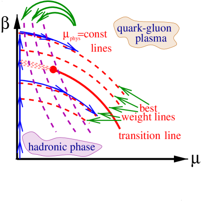
Figure 10: Illustration of the integral method at finite chemical potential (left panel). The solid lines are $\mu={\rm const}$ lines on the $\mu a-\beta$ plane. Dashed lines are the best reweighting lines starting from different simulation points. Arrows show the path of integration we used when evaluating eq. (7.7).

For the pressure we have an additional variable in the integral, the gradient of $\log Z_{gc}$ has now an extra component in the $a\mu$ direction:

$$\frac{p}{T^{4}}=-\frac{N_{t}^{3}}{N_{s}^{3}}\int^{(\beta,am_{i},a\mu)}_{(\beta_{0},am_{i0},a\mu=0)}d(\beta,am_{i},a\mu)\left(\begin{array}[]{c}{\partial\log Z_{gc}}/{\partial\beta}\\ {\partial\log Z_{gc}}/{\partial(am_{i})}\\ {\partial\log Z_{gc}}/{\partial(a\mu)}\end{array}\right)-\frac{p_{0}}{T^{4}}.$$ (23)

The subtracted $p_{0}$ term is now the pressure at $T=0$ and $\mu=0$, i.e. the same as before. We can rewrite the above equation in terms of observables:

$$\frac{p}{T^{4}} = -N_{t}^{4}\int^{(\beta,am_{i},a\mu)}_{(\beta_{0},am_{i0},a\mu=0)}d(\beta,am_{ud},am_{s},a\mu)\left(\begin{array}[]{ll}&\langle{\rm Pl}\rangle^{(\mu)}\\ &\langle\bar{\Psi}\Psi_{ud}\rangle^{(\mu)}\\ &\langle\bar{\Psi}\Psi_{s}\rangle^{(\mu)}\\ {N_{s}^{3}N_{t}}^{-1}&\langle{\frac{\partial\log\det M}{\partial(a\mu)}\rangle^{(\mu)}}\end{array}\right)$$ (28)

where the superscript $\mu$ denotes the expectation values of the observables at reweighted $\mu$ values:

$$\langle{\cal O}(\beta,\mu,m)\rangle^{(\mu)}={\overline{{\cal{O}}}(\beta,\mu,m)}_{T\neq 0}-{\overline{{\cal O}}(\beta,\mu=0,m)}_{T=0}.$$ (30)

The result should again be independent of the integration path. We chose the following paths (cf. Fig. 10). First we integrated from ($\beta_{0}$, $am_{i0}$) to some ($\beta_{1}$, $am_{i1}$) along the LCP with $\mu=0$. Then we followed the line of best reweighting to reach the required ($\beta$, $am_{i}$, $a\mu$) point. We checked that the result remains unchanged if we do it in the opposite way, i.e. we go first along the best reweighting line and then along the constant $a\mu$ line. The results along the two integration lines were equal within statistical errors.

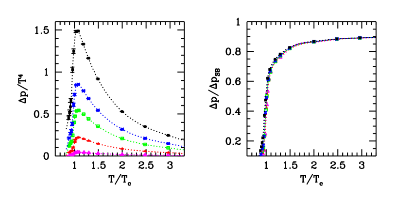
Figure 11: The equation of state at, $\mu_{B}=100$, 210, 330, 410 and 530 MeV. The left panel shows the pressure difference between the $\mu=0$ and $\mu\neq 0$ cases normalized by $T^{4}$, whereas on the right panel the normalization is done by the $N_{t}=4$ lattice Stefan-Boltzman limit (in continuum this limit is $n_{f}(\mu/T)^{2}$). Note that $\Delta p/\Delta p^{SB}$ seems to show some scaling behaviour (it depends mostly on the temperature; whereas its dependence on $\mu$ is much weaker). Thus, the $\mu$ dependence of $\Delta p$ is almost completely given by the $\mu$ dependence of the free gas.

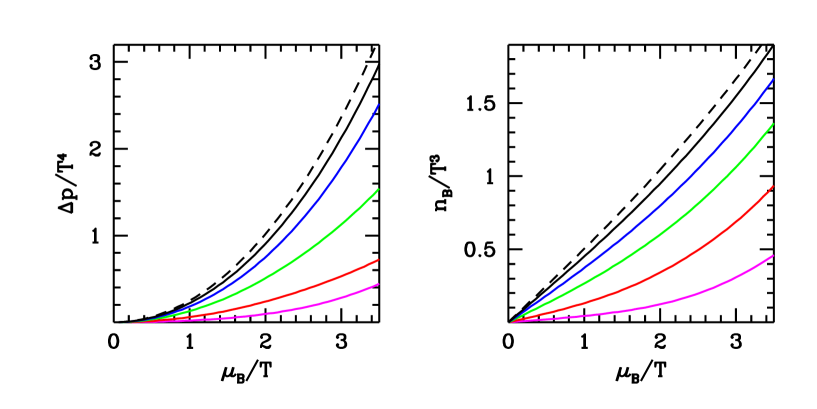
Figure 12: (a) The difference of the pressure at finite $\mu_{B}$ and $\mu_{B}=0$ (left panel) as a function of $\mu_{B}/T$ at $T/T_{c}=0.9$, 0.98, 1.03, 1.2, 2.28. (b) Dimensionless baryon number density as a function of $\mu_{B}$ at $T/T_{c}=0.9$, 0.98, 1.03, 1.2, 2.48. Dashed line shows the SB limit in both cases. The higher the temperature is, the closer the lines run to the SB limit.

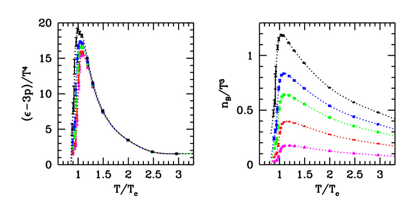
Figure 13: (a) $(\epsilon-3p)/T^{4}$ (b) Dimensionless baryon number density as a function of $T/T_{c}$ at $\mu_{B}$=100,210,330,410 MeV and $\mu_{B}$=530 MeV.

We present lattice results on $\Delta p(\mu,T)=p(\mu\neq 0,T)-p(\mu=0,T)$, $\epsilon(\mu,T)$-3$p(\mu,T)$ and $n_{B}(\mu,T)$. Our statistical errorbars are also shown. They are rather small, in many cases they are even smaller than the thickness of the lines.

On the left panel of Fig. 11 we present $\Delta p/T^{4}$ for five different $\mu$ values. On the right panel normalisation is done by $\Delta p^{SB}$, which is $\Delta p(\mu,T\rightarrow\infty)$. Notice the interesting scaling behaviour. $\Delta p/\Delta p^{SB}$ depends only on T and it is practically independent from $\mu$ in the analysed region. The left panel of Fig. 12 shows the same pressure difference as a function of $\mu_{B}/T$ for five different temperatures. The right panel shows dimensionless baryon number density ($n_{B}/T^{3}$) as a function of $\mu_{B}/T$ at the same temperatures. The left panel of Fig. 13 shows $\epsilon$-3$p$ normalised by $T^{4}$, which tends to zero for large $T$. The right panel of Fig. 13 gives the dimensionless baryonic density as a function of $T/T_{c}$ for different $\mu$-s.

Here we summarise what kind of errors occur during our lattice calculations. The error coming from reweighting has been amply discussed in Section 5. Another source of error is the finiteness of the physical volume. The volume dependence of physical observables is smaller than the statistical errors for the plaquette average or quark number density. Systematic errors coming from non-zero microcanonical step-size cause a 0.2% and 0.1% error in the value of physical observables for zero temperature and finite temperature calculations, respectively.

8 Conclusions, outlook

In this paper we studied the thermodynamical properties of QCD at finite chemical potential $\mu$. We used the overlap enhancing multi-parameter reweighting method proposed by two of us [17] and its generalization to $2+1$ flavour staggered QCD [21]. Our primary goal was to determine the equation of state (EoS) on the line of constant physics (LCP) at finite temperature and chemical potential.

We have pointed out that even at $\mu$=0 the EoS depends on the fact whether we are on an LCP or not. Note that previous results in the staggered formalism usually used the “non-LCP approach”. According to our findings pressure and $\epsilon$ - 3p (interacion measure) on the LCP has different high temperature behaviour than in the “non-LCP approach”.

We discussed the reliability of the reweighting technique. We introduced an error estimate, which successfully shows the limits of the method yielding infinite errors in the parameter regions, where reweighting gives wrong results. We showed how to define and determine the best weight lines on the $\mu$–$\beta$ plane.

We discussed the two-parameter and three-parameter reweighting techniques. Two techniques were presented (three-parameter reweighting and the interpolating method) to stay on the LCP even when reweighting to non-vanishing chemical potentials.

We calculated the thermodynamic equations for $\mu\neq 0$ and determined the EoS along an LCP. We presented lattice data on the pressure, the interaction-measure and the baryon number density as a function of temperature and chemical potential. The physical range of our analysis extended upto $500-600$ MeV in temperature and baryon chemical potential as well.

Clearly much more work is needed to get the final form of non-perturbative EoS of QCD. One has to extrapolate to zero step-size in the R-algorithm. Extrapolation to the thermodynamic and continuum limits is a very CPU demanding task in the $\mu\neq 0$ case. Physical $m_{\pi}/m_{\rho}$ ratio should be reached by decreasing the light quark mass. Finally, renormalised LCP’s (LCP^∗ in our notation) should be used when evaluating thermodynamic quantites.

9 Acknowledgements

This work was partially supported by Hungarian Scientific grants, OTKA-T37615/T34980/T29803/M37071/OMFB1548/OMMU-708. For the simulations a modified version of the MILC public code was used (see http://physics.indiana.edu/~sg/milc.html). The simulations were carried out on the Eötvös Univ., Inst. Theor. Phys. 163 node parallel PC cluster.

References

- [1] F. Wilczek, arXiv:hep-ph/0003183.
- [2] M. G. Alford, K. Rajagopal and F. Wilczek, Phys. Lett. B 422 (1998) 247 [arXiv:hep-ph/9711395].
- [3] M. G. Alford, K. Rajagopal and F. Wilczek, Nucl. Phys. B 537 (1999) 443 [arXiv:hep-ph/9804403].
- [4] R. Rapp, T. Schafer, E. V. Shuryak and M. Velkovsky, Phys. Rev. Lett. 81 (1998) 53 [arXiv:hep-ph/9711396].
- [5] for a recent review see K. Rajagopal and F. Wilczek, arXiv:hep-ph/0011333.
- [6] A. Ukawa, Nucl. Phys. Proc. Suppl. 53 (1997) 106 [arXiv:hep-lat/9612011].
- [7] E. Laermann, Nucl. Phys. Proc. Suppl. 63 (1998) 114 [arXiv:hep-lat/9802030].
- [8] F. Karsch, Nucl. Phys. Proc. Suppl. 83 (2000) 14 [arXiv:hep-lat/9909006].
- [9] S. Ejiri, Nucl. Phys. Proc. Suppl. 94 (2001) 19 [arXiv:hep-lat/0011006].
- [10] J. B. Kogut, Nucl. Phys. Proc. Suppl. 119, (2003) 210 [arXiv:hep-lat/0208077];
- [11] Z. Fodor, Nucl. Phys. A 715, (2003) 319 [arXiv:hep-lat/0209101];
- [12] E. Laermann and O. Philipsen, arXiv:hep-ph/0303042;
- [13] S. Muroya, A. Nakamura, C. Nonaka and T. Takaishi, Prog. Theor. Phys. 110, (2003) 615 [arXiv:hep-lat/0306031];
- [14] S. D. Katz, hep-lat/0310051.
- [15] P. Hasenfratz and F. Karsch, Phys. Lett. B 125 (1983) 308.
- [16] J. B. Kogut, H. Matsuoka, M. Stone, H. W. Wyld, S. H. Shenker, J. Shigemitsu and D. K. Sinclair, Nucl. Phys. B 225 (1983) 93.
- [17] Z. Fodor and S. D. Katz, Phys. Lett. B 534 (2002) 87, [arXiv:hep-lat/0104001].
- [18] A. M. Ferrenberg and R. H. Swendsen, Phys. Rev. Lett. 61 (1988) 2635.
- [19] A. M. Ferrenberg and R. H. Swendsen, Phys. Rev. Lett. 63 (1989) 1195.
- [20] I. M. Barbour, S. E. Morrison, E. G. Klepfish, J. B. Kogut and M. P. Lombardo, Nucl. Phys. Proc. Suppl. 60A (1998) 220 [arXiv:hep-lat/9705042].
- [21] Z. Fodor and S. D. Katz, JHEP 0203 (2002) 014 [arXiv:hep-lat/0106002].
- [22] F. Csikor, Z. Fodor and J. Heitger, Phys. Rev. Lett. 82 (1999) 21 [arXiv:hep-ph/9809291].
- [23] Y. Aoki, F. Csikor, Z. Fodor and A. Ukawa, Phys. Rev. D 60 (1999) 013001 [arXiv:hep-lat/9901021].
- [24] S. Choe et al., Phys. Rev. D 65 (2002) 054501.
- [25] C. R. Allton et al., Phys. Rev. D 66 (2002) 074507 [arXiv:hep-lat/0204010].
- [26] C. R. Allton, S. Ejiri, S. J. Hands, O. Kaczmarek, F. Karsch, E. Laermann, C. Schmidt Phys. Rev. D 68 (2003) 014507; [arXiv:hep-lat/0305007].
- [27] R. V. Gavai and S. Gupta, Phys. Rev. D 68 (2003) 034506 [arXiv:hep-lat/0303013].
- [28] P. de Forcrand and O. Philipsen, Nucl. Phys. B 642 (2002) 290 [arXiv:hep-lat/0205016].
- [29] P. de Forcrand and O. Philipsen, Nucl. Phys. B 673, (2003) 170 [arXiv:hep-lat/0307020].
- [30] M. D’Elia and M. P. Lombardo, Phys. Rev. D 67, (2003) 014505 [arXiv:hep-lat/0209146].
- [31] C. W. Bernard et al. [MILC Collaboration], Phys. Rev. D 55 (1997) 6861 [arXiv:hep-lat/9612025].
- [32] J. Engels, R. Joswig, F. Karsch, E. Laermann, M. Lutgemeier and B. Petersson, Phys. Lett. B 396 (1997) 210 [arXiv:hep-lat/9612018].
- [33] F. Karsch, E. Laermann and A. Peikert, Phys. Lett. B 478 (2000) 447 [arXiv:hep-lat/0002003].
- [34] J. Engels, J. Fingberg, F. Karsch, D. Miller and M. Weber, Phys. Lett. B 252 (1990) 625.
- [35] Z. Fodor, S. D. Katz and K. K. Szabo, Phys. Lett. B 568 (2003) 73 [arXiv:hep-lat/0208078].
- [36] F. Csikor, G. I. Egri, Z. Fodor, S. D. Katz, K. K. Szabo and A. I. Toth, arXiv:hep-lat/0209114.
- [37] C. Michael and A. McKerrell, Phys. Rev. D 51 (1995) 3745 [arXiv:hep-lat/9412087].
- [38] S. Gottlieb, W. Liu, D. Toussaint, R. L. Renken and R. L. Sugar, Phys. Rev. D 35 (1987) 2531.
- [39] T. Blum, L. Karkkainen, D. Toussaint and S. Gottlieb, Phys. Rev. D 51 (1995) 5153 [arXiv:hep-lat/9410014].
- [40] G. Boyd, J. Engels, F. Karsch, E. Laermann, C. Legeland, M. Lutgemeier and B. Petersson, Nucl. Phys. B 469 (1996) 419 [arXiv:hep-lat/9602007].
- [41] M. Okamoto et al. [CP-PACS Collaboration], Phys. Rev. D 60 (1999) 094510 [arXiv:hep-lat/9905005].
- [42] B. Beinlich, F. Karsch, E. Laermann and A. Peikert, Eur. Phys. J. C 6 (1999) 133 [arXiv:hep-lat/9707023].
- [43] S. Ejiri, Y. Iwasaki and K. Kanaya, Phys. Rev. D 58 (1998) 094505 [arXiv:hep-lat/9806007].
- [44] J. Engels, F. Karsch and T. Scheideler, Nucl. Phys. B 564 (2000) 303 [arXiv:hep-lat/9905002].
- [45] R. Sommer, Nucl. Phys. B 411 (1994) 839 [arXiv:hep-lat/9310022].
- [46] C. W. Bernard et al., Phys. Rev. D 64 (2001) 054506 [arXiv:hep-lat/0104002].
- [47] C. R. Allton, arXiv:hep-lat/9610016.
- [48] A. Ali Khan et al. [CP-PACS collaboration], Phys. Rev. D 64 (2001) 074510 [arXiv:hep-lat/0103028].
- [49] S. Ejiri, arXiv:hep-lat/0401012.
- [50] Ferrenberg, Landau, Swendsen Phys. Rev. E 51 (1995) 5092-5100
- [51] M. E. J. Newman, R. G. Palmer J. Stat. Phys. 97 (1999) 1011-1026