Finite Temperature QCD with Two Flavors of Non-perturbatively Improved Wilson Fermions

Abstract:

We study QCD with two flavors of non-perturbatively improved Wilson fermions at finite temperature on the $16^{3}\,8$ lattice. We determine the transition temperature at lattice spacings as small as $a\sim 0.12$ fm, and study string breaking below the finite temperature transition. We find that the static potential can be fitted by a two-state ansatz, including a string state and a two-meson state. We investigate the role of Abelian monopoles at finite temperature.

1 Introduction

Recently, efforts have been made to determine the critical temperature $T_{c}$ of the finite temperature transition in full QCD with $N_{f}=2$ flavors of dynamical quarks. The Bielefeld group employed improved staggered fermions and an improved gauge field action [1]. The CP-PACS collaboration used improved Wilson fermions with mean field improved clover coefficient and an improved gauge field action [2]. Both groups were able to estimate $T_{c}$ in the chiral limit, and their values are in good agreement with each other. Still, there are many sources of systematic uncertainties. The main one is that the lattices used so far are rather coarse. In this paper we perform simulations on $N_{s}^{3}\,N_{t}=16^{3}\,8$ lattices at lattice spacings $a$ much smaller than in previous works [1, 2]. To further reduce finite cut-off effects, we use non-perturbatively $O(a)$ improved Wilson fermions. A small lattice spacing is particularly helpful in determining the parameters of the static potential.

In the presence of dynamical quarks the flux tube formed between static quark-antiquark pairs is expected to break at large distances. At zero temperature $T$ the search for string breaking, i.e. flattening of the static potential, has not been successful, if the static quarks are created by the Wilson loop. (See e.g. [3]). At finite temperature string breaking has been observed at $T<T_{c}$, if Polyakov loops are used instead to create the quarks. It is important to know the static potential at finite temperature for phenomenology [4]. In particular, it is needed to compute the dissociation temperatures for heavy quarkonia. We suggest a new ansatz and confront that ansatz with our numerical data.

The dynamics of the QCD vacuum, and color confinement in particular, becomes more transparent in the maximally Abelian gauge (MAG) [5, 6]. In this gauge the relevant degrees of freedom are color electric charges, color magnetic monopoles, ‘photons’ and ‘gluons’ [7]. There is evidence that the monopoles condense in the low temperature phase of the theory [6, 8], causing a dual Meissner effect, which constricts the color electric field into flux tubes, in accord with the dual superconductor picture of confinement [9]. Abelian dominance [10] and the dynamics of monopoles have been studied in detail at zero temperature in quenched [11] and unquenched [12, 13] lattice simulations. It turns out that in MAG the string tension is accounted for almost entirely by the monopole part of the Abelian projected gauge field [14, 15, 16, 12]. Furthermore, in studies of SU(2) gauge theory at nonzero temperature [17] it has been found that at the phase transition the Abelian Polyakov loop shows qualitatively the same behavior as the non-Abstain one. In this paper we extend the investigation of Abelian dominance to full QCD at nonzero temperature.

The paper is organized as follows. In Section 2 we present the details of our simulation. Furthermore, we describe the gauge fixing algorithm and the Abelian projection. Section 3 is devoted to the determination of the transition temperature, and in Section 4 our results for the heavy quark potential are presented. In Section 5 we study the monopole density in the vacuum, as well as the action density in the vicinity of the flux tube. We demonstrate that the flux tube disappears at large quark-antiquark separations. Finally, in Section 6 we conclude. Preliminary results of this work have been reported in [18].

2 Simulation details

We consider $N_{f}=2$ flavors of degenerate quarks. We use the Wilson gauge field action and non-perturbatively $O(a)$ improved Wilson fermions [19]

$$S_{F}=S^{(0)}_{F}-\frac{\rm i}{2}\kappa\,g\,c_{sw}a^{5}\sum_{s}\bar{\psi}(s)\sigma_{\mu\nu}F_{\mu\nu}(s)\psi(s),$$ (1)

where $S^{(0)}_{F}$ is the original Wilson action, $g$ is the gauge coupling and $F_{\mu\nu}(x)$ is the field strength tensor. The clover coefficient $c_{sw}$ is determined non-perturbatively. This action has been used in simulations of full QCD at zero temperature by the QCDSF and UKQCD collaborations [20, 21], whose results we use to fix the physical scale and the $m_{\pi}/m_{\rho}$ ratio. At finite temperature the same action was used before in simulations on $N_{t}=4$ and 6 lattices at rather large quark masses and lattice spacings [22].

Non-perturbatively improved $N_{f}=2$ Wilson fermions should not be employed below $\beta\equiv 6/g^{2}=5.2$. In fact, $c_{sw}$ is known only for $\beta\geq 5.2$ [23]. The simulations are done on $16^{3}\,8$ lattices at two values of the coupling constant, $\beta=5.2$ and 5.25, and nine different $\kappa$ values each. The parameters are listed in Table 1. They are also shown in Fig. 1, together with lines of constant $r_{0}/a$ and constant $m_{\pi}/m_{\rho}$ obtained at $T=0$ [20]. Note that the lines of constant $T$ run parallel to the lines of constant $r_{0}/a$. To check the finite size effects we have also done simulations on the $24^{3}\,8$ lattice at $\beta=5.2$, $\kappa=0.1343$.

The dynamical gauge field configurations are generated on the Hitachi SR8000 at KEK (Tsukuba) and on the MVS 1000M at Joint Supercomputer Center (Moscow), using a Hybrid Monte Carlo , while the analysis is done on the NEC SX5 at RCNP (Osaka) and on the PC-cluster at ITP (Kanazawa). Our present statistics is shown in Table 1. The length of the trajectory was chosen to be $\tau=0.25$. We use a blocked jackknife method to compute the statistical errors of the observables and a bootstrap method to compute the errors of the fit parameters.

Figure 1: Lines of constant $r_{0}/a$ (solid lines) and constant $m_{\pi}/m_{\rho}$ (dotted lines) at $T=0$. Crosses indicate points where simulations are done.

$\beta=5.2$			$\beta=5.25$
$\kappa$	Trajectories	$\tau_{int}$	$\kappa$	Trajectories	$\tau_{int}$
0.1330	7129	24	0.1330	1800	11
0.1335	4500	54	0.1335	7500	90
0.1340	3000	62	0.13375	9225	200
0.1343	6616	240	0.1339	12470	440
0.1344	8825	520	0.1340	19800	700
0.1345	6877	190	0.1341	14800	700
0.1348	5813	124	0.13425	5155	120
0.1355	5650	50	0.1345	2650	50
0.1360	3699	46	0.1350	1780	30

Table 1: Parameters and statistics of the simulation, together with the integrated autocorrelation time. The length of the trajectory is $\tau=0.25$.

We compute the Polyakov loop

$$L(\vec{s})=\frac{1}{3}\mathop{\rm Tr}\prod_{s_{4}=1}^{N_{t}}U(s,4),$$ (2)

$U(s,\mu)$ being the link variable, on every trajectory. From that we derive the susceptibility

$$\chi=N_{s}^{3}\sum_{\vec{s}}(\langle L^{2}(\vec{s})\rangle-\langle L(\vec{s})\rangle^{2}),$$ (3)

and the integrated autocorrelation time $\tau_{int}$. The autocorrelation time is given in Table 1 in units of trajectories. Furthermore, we compute the Polyakov loop correlator $\langle L(\vec{s})L^{\dagger}(\vec{s}\,^{\prime})\rangle$, from which we obtain the static potential. To reduce the error on the static potential, we employ a hypercubic blocking of the gauge field as described in [24]. We choose every $5^{th}$ to $20^{th}$ trajectory, depending on the value of $\kappa$, to compute the blocked Polyakov loop correlator.

We fix the MAG  [6] by maximizing the gauge fixing functional $F(U)$,

$$F(U)=\frac{1}{12V}\sum_{s,\mu}(|U_{11}(s,\mu)|^{2}+|U_{22}(s,\mu)|^{2}+|U_{33}(s,\mu)|^{2})$$ (4)

with respect to local gauge transformations $g$ of the lattice gauge field,

$$U(s,\mu)\rightarrow U^{g}(s,\mu)=g(s)^{\dagger}U(s,\mu)g(s+\hat{\mu})\,.$$ (5)

To do so, we use the simulated annealing (SA) algorithm. The advantage of this algorithm over the usual iterative procedure has been demonstrated in [16] for the MAG and in [25] for the maximal center gauge in the SU(2) gauge theory. In practice one does not find the global maximum of the gauge fixing functional in a finite-time computation. For this reason it has been proposed [16] to apply the SA algorithm to a number of randomly generated gauge copies and pick that one with the largest value of $F$. By increasing the number of gauge copies, one eventually reaches the situation, where the statistical noise is larger than the deviation from the global maximum. We use one gauge copy at $\beta=5.2$ and three gauge copies at $\beta=5.25$. We have checked that by increasing the number of gauge copies our results for the gauge dependent quantities are left unchanged within the error bars.

To obtain Abelian observables, one needs to project the $SU(3)$ link matrices onto the maximal Abelian subgroup $U(1)\times U(1)$ first. The original construction [26] is equivalent to finding the Abelian gauge field $u(s,\mu)\in U(1)\times U(1)$ which maximizes $|\mbox{Tr}\left(U(s,\mu)u^{\dagger}(s,\mu)\right)|^{2}$. The Abelian counterpart of an observable is then obtained by substituting

$$u(s,\mu)=\mathrm{diag}(e^{{\rm i}\theta_{1}(s,\mu)},e^{{\rm i}\theta_{2}(s,\mu)},e^{{\rm i}\theta_{3}(s,\mu)})\,,$$ (6)

for $U(s,\mu)$; $\sum_{i=1}^{3}\theta_{i}(s,\mu)=0$, so that $\det(u(s,\mu))=1$. From eq. (6) we define plaquette angles

$$\theta_{i}(s,\mu\nu)=\partial_{\mu}\theta_{i}(s,\nu)-\partial_{\nu}\theta_{i}(s,\mu)\,,$$ (7)

where $\partial_{\mu}$ is the lattice forward derivative. The plaquette angles can be decomposed into regular and singular components,

$$\theta_{i}(s,\mu\nu)=\overline{\theta}_{i}(s,\mu\nu)+2\pi m_{i}(s,\mu\nu)\,,$$ (8)

where $\overline{\theta}_{i}(s,\mu\nu)\in(-\pi;\pi]$, and $m_{i}(s,\mu\nu)\in\mathbb{N}$ counts the number of Dirac strings piercing the given plaquette. Note that $\sum_{i}\overline{\theta}_{i}(s,\mu\nu)=2\pi l$, $l=0,\pm 1$. If $l=+1$ ($-1$) we substitute the largest (smallest) $\overline{\theta}_{i}(s,\mu\nu)$ (of the three components) by $\overline{\theta}_{i}(s,\mu\nu)-2\pi$ ($+2\pi$), and similarly for $m_{i}(s,\mu\nu)$, so that $\sum_{i}\overline{\theta}_{i}(s,\mu\nu)=\sum_{i}m_{i}(s,\mu\nu)=0$.

The monopole currents, being located on the links of the dual lattice, are defined by [27]

$$k_{i}(^{*}s,\mu)=\frac{1}{4\pi}\epsilon_{\mu\nu\rho\sigma}\partial_{\nu}\overline{\theta}_{i}(s+\hat{\mu},\rho\sigma)=-\frac{1}{2}\epsilon_{\mu\nu\rho\sigma}\partial_{\nu}m_{i}(s+\hat{\mu},\rho\sigma)\,.$$ (9)

They satisfy the constraint

$$\sum_{i}k_{i}(^{*}s,\mu)=0\,,$$ (10)

for any ${}^{*}s,\mu$. The Abelian gauge fields $\theta_{i}(s,\mu)$ can in turn be decomposed into monopole (singular) and photon (regular) parts:

$$\theta_{i}(s,\mu)=\theta^{\rm mon}_{i}(s,\mu)+\theta^{\rm ph}_{i}(s,\mu)\,.$$ (11)

The monopole part is defined by [28]:

$$\theta^{\rm mon}_{i}(s,\mu)=-2\pi\sum_{s^{\prime}}D(s-s^{\prime})\,\partial_{\nu}^{\prime}\,m_{i}(s^{\prime},\nu\mu)\,,$$ (12)

where $\partial_{\nu}\,^{\prime}$ is the backward lattice derivative, and $D(s)$ denotes the lattice Coulomb propagator.

The Abelian Polyakov loop is defined by

$$L_{\rm Abel}(\vec{s})=\frac{1}{3}\sum_{i=1}^{3}L^{\rm Abel}_{i}(\vec{s})\,,\qquad L^{\rm Abel}_{i}(\vec{s})=\exp\Bigl{\{}{\rm i}\sum_{s_{4}=1}^{N_{t}}\theta_{i}(s,4)\Bigr{\}}\,.$$ (13)

Similarly, we define the monopole and photon Polyakov loops [29]:

$$L_{\rm mon}(\vec{s})=\frac{1}{3}\sum_{i=1}^{3}L^{\rm mon}_{i}(\vec{s})\,,\qquad L^{\rm mon}_{i}(\vec{s})=\exp\Bigl{\{}{\rm i}\sum_{s_{4}=1}^{N_{t}}\theta_{i}^{\rm mon}(s,4)\Bigr{\}}\,,$$ (14)

$$L_{\rm ph}(\vec{s})=\frac{1}{3}\sum_{i=1}^{3}L^{\rm ph}_{i}(\vec{s})\,,\qquad L^{\rm ph}_{i}(\vec{s})=\exp\Bigl{\{}{\rm i}\sum_{s_{4}=1}\theta_{i}^{\rm ph}(s,4)\Bigr{\}}\,.$$ (15)

3 Transition temperature

The order parameter of the finite temperature phase transition in quenched QCD is the Polyakov loop, and the corresponding symmetry is global $Z(3)$. In the presence of dynamical ‘chiral’ fermions the chiral condensate $\langle\bar{\psi}\psi\rangle$ is an order parameter (of the chiral symmetry breaking transition). It is expected that there is no phase transition at intermediate quark masses, only a crossover. Numerical results show that both order parameters can be used to locate the transition point at intermediate quark masses [1]. We use the Polyakov loop, because the calculation of the chiral condensate for Wilson fermions requires renormalization and is rather involved.

It is instructive to plot the Polyakov loop in the complex plane as a function of temperature, which has been done in Fig. 2. We find that the distribution is rather asymmetric, even at the lowest temperature, favoring a positive value of ${\rm Re}\,L$. This is indeed what one expects [30]. The introduction of dynamical quarks adds a term proportional to ${\rm Re}\,L$ to the effective action, which results in a nonzero value of ${\langle L\rangle}$. The numbers are given in Tables 2 and 3. In the Tables we also give values for the Abelian and monopole Polyakov loops separately.

Figure 2: Scatter plots of the Polyakov loop in the complex plane for various temperatures.

$\kappa$	${\langle L\rangle}$	${\langle L\rangle}_{\rm Abel}$	${\langle L\rangle}_{\rm mon}$	${\langle L\rangle}_{\rm ph}$	$T/T_{c}$
0.1330	0.0022(3)	0.014(2)	0.040(7)	0.2946(10)	0.80
0.1335	0.0027(7)	0.018(5)	0.054(16)	0.3007(9)	0.87
0.1340	0.0034(5)	0.025(4)	0.079(14)	0.3052(7)	0.94
0.1343	0.0092(13)	0.074(11)	0.235(35)	0.3113(6)	0.98
0.1344	0.0131(18)	0.107(15)	0.352(51)	0.3136(6)	1.00
0.1345	0.0120(12)	0.098(10)	0.319(33)	0.3145(5)	1.02
0.1348	0.0207(11)	0.169(10)	0.556(32)	0.3197(9)	1.06
0.1355	0.0300(7)	0.235(5)	0.740(11)	0.3279(9)	1.18
0.1360	0.0290(9)	0.236(6)	0.747(11)	0.3291(14)	1.28

Table 2: The expectation values of the non-Abelian, Abelian, monopole and photon Polyakov loops at $\beta=5.2$.

As we can see from Fig. 1, increasing $\kappa$ at a fixed value of $\beta$ increases the temperature $T\propto r_{0}/a$. In Figs. 3, 4, 5 we plot the expectation values of the various Polyakov loops of Tables 2 and 3 as a function of $\kappa$. While $\langle L\rangle$, $\langle L_{\mathrm{Abel}}\rangle$ and $\langle L_{\mathrm{mon}}\rangle$ increase with increasing $\kappa$, $\langle L_{\mathrm{ph}}\rangle$ stays approximately constant over the full range of $\kappa$. Furthermore, similar to the quenched theory, $L_{\mathrm{mon}}$ and $L_{\mathrm{ph}}$ are virtually independent, which follows from $\langle L_{\mathrm{Abel}}\rangle\approx\langle L_{\mathrm{mon}}\rangle\langle L_{\mathrm{ph}}\rangle$. We have no explanation for the dip seen in $\langle L\rangle$ at $\beta=5.25$ around $\kappa=0.1341$. We see some signal of metastability, but we will need higher statistics to clarify this point. A similar dip is seen on Fig. 1 of ref. [22], where the same lattice action was used to study the phase transition on small lattices.

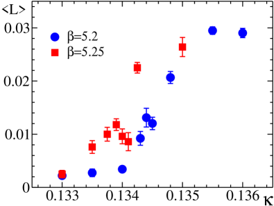
Figure 3: The expectation value of the non-Abelian Polyakov loop as a function of $\kappa$ for $\beta=5.2$ and 5.25.

$\kappa$	${\langle L\rangle}$	${\langle L\rangle}_{\mathrm{mon}}$	$T/T_{c}$
0.1330	0.0025(7)	0.060(13)	0.86
0.1335	0.0076(12)	0.188(30)	0.92
0.13375	0.0100(13)	0.273(35)	0.96
0.1339	0.0118(11)	0.321(35)	0.97
0.1340	0.0096(14)	0.248(40)	0.99
0.1341	0.0086(17)	0.230(50)	1.00
0.13425	0.0225(10)	0.604(22)	1.02
0.1345	0.0255(9)	–	1.05
0.1350	0.0264(18)	0.706(25)	1.12

Table 3: The expectation values of the non-Abelian and monopole Polyakov loops at $\beta=5.25$.

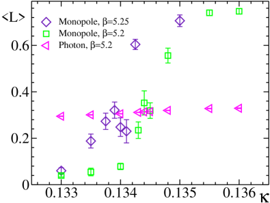
Figure 4: The expectation value of monopole and photon Polyakov loops as functions of $\kappa$ for $\beta=5.2$ and 5.25.

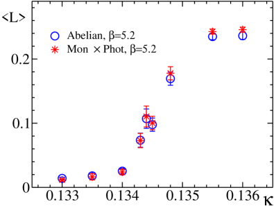
Figure 5: The expectation value of the Abelian Polyakov loop as a function of $\kappa$ for $\beta=5.2$. The product of monopole and photon Polyakov loops is also shown.

The task is now to determine the transition temperature $T_{c}$. We call the $\kappa$ value, at which the transition takes place, $\kappa_{t}$. We identify $\kappa_{t}$ as the point, where the Polyakov loop susceptibility (3) assumes its maximum. The Abelian, monopole and photon Polyakov susceptibilities $\chi_{\rm Abel}$, $\chi_{\rm mon}$ and $\chi_{\rm ph}$, respectively, are defined similarly. The susceptibilities are given in Tables 4 and 5, and they are plotted in Figs. 6 and 7. From the non-Abelian susceptibility $\chi$ we find $\kappa_{t}=0.1344(1)$ at $\beta=5.2$ and $\kappa_{t}=0.1341(1)$ at $\beta=5.25$ where the central values and the errors are determined by the maxima of susceptibilities and by the distances to neighbor data points, respectively

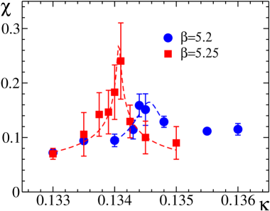
Figure 6: The non-Abelian Polyakov loop susceptibility as a function of $\kappa$ for $\beta=5.2$ and 5.25, respectively, together with the fit.

$\kappa$	$\chi$	$\chi_{\mathrm{Abel}}$	$\chi_{\mathrm{mon}}$	$\chi_{\mathrm{ph}}$
0.1330	0.072(3)	0.88(10)	7.7(8)	0.590(16)
0.1335	0.094(5)	1.8(3)	17.4(2.4)	0.624(10)
0.1340	0.095(12)	2.4(5)	25.5(4.9)	0.638(12)
0.1343	0.115(17)	4.2(1.1)	46.1(12.)	0.653(10)
0.1344	0.159(21)	7.7(1.5)	88.4(20.)	0.682(13)
0.1345	0.151(29)	6.6(1.5)	70.4(14.)	0.671(16)
0.1348	0.129(10)	5.7(8)	57.5(9.4)	0.705(25)
0.1355	0.112(5)	2.7(4)	17.7(2.2)	0.686(27)
0.1360	0.115(11)	2.3(5)	14.7(2.8)	0.734(29)

Table 4: The same as in Table 3 but for the susceptibility of the Polyakov loop at $\beta=5.2$.

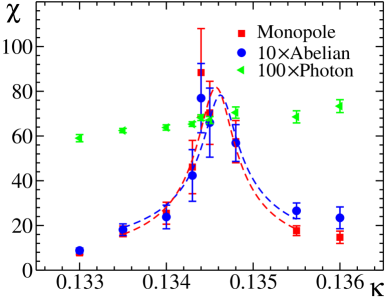
Figure 7: The same as in Fig. 6 but for the Abelian, the monopole and the photon Polyakov loop susceptibilities. The Abelian (photon) Polyakov loop susceptibility has been enhanced by a factor of 10 (100).

$\kappa$	$\chi$	$\chi_{\mathrm{mon}}$
0.1330	0.07(1)	15(5)
0.1335	0.11(4)	65(15)
0.13375	0.14(4)	105(25)
0.1339	0.15(4)	75(20)
0.1340	0.18(5)	106(22)
0.1341	0.24(7)	150(30)
0.13425	0.13(3)	37(10)
0.1345	0.10(3)	–
0.1350	0.09(3)	53(18)

Table 5: The same as in Table 4 but for the susceptibility of the Polyakov loop at $\beta=5.25$.

This translates into $T_{c}r_{0}=0.53(1)$ at $\beta=5.2$ and $T_{c}r_{0}=0.56(1)$ at $\beta=5.25$, where the numbers of $r_{0}/a$ at $\kappa_{t}$ have been obtained by interpolation of the $T=0$ results [20]. Taking $r_{0}=0.5$ fm to fix the scale, we obtain in physical units

$$T_{c} = 210(3)~{}{\rm MeV},\,\,\,\beta=5.2$$ (16)

$$T_{c} = 219(3)~{}{\rm MeV},\,\,\,\beta=5.25\,.$$

By interpolating $m_{\pi}/m_{\rho}$, given in [20], to $\kappa_{t}$ we obtain at the transition point $m_{\pi}/m_{\rho}=0.77$ at $\beta=5.2$ and $0.81$ at $\beta=5.25$. Similarly, we can compute the temperature $T$ at our various $\kappa$ values. The result is given in the last column of Table 2 and Table 3 in the form of $T/T_{c}$.

The susceptibilities $\chi_{\rm Abel}$ and $\chi_{\rm mon}$ have maxima at the same $\kappa$ value as the non-Abelian susceptibility. We find that $\chi_{\rm Abel}\approx\langle L_{\rm ph}\rangle^{2}\chi_{\rm mon}$. This follows from our earlier observation, namely that $L_{\rm mon}$ and $L_{\rm ph}$ are independent, and the smallness of $\chi_{\mathrm{ph}}$. The non-Abelian susceptibility is 10 to 50 times smaller than its Abelian counterpart. The photon susceptibility does not show any change at the critical temperature, as expected. We conclude, that the monopole degrees of freedom are most sensitive to the transition, as was the case in the quenched theory.

In Fig. 8 we compare our results for $T_{c}$ with those of Refs. [1] and [22], where we have assumed $\sqrt{\sigma}=425$ MeV. Our results are in quantitative agreement with the results of the Bielefeld group. This is reassuring, as [1] and [22] work at larger lattice spacing.

Figure 8: The transition temperature as a function of $m_{\pi}/m_{\rho}$ from this work (triangles), and from [1] (squares) and [22] (circle), respectively.

$\beta$	$5.2$			$5.25$
$\chi$	non-Abelian	Abelian	monopole	non-Abelian
$\kappa_{t}$	0.13457(8)	0.13459(5)	0.13457(4)	0.13407(2)
$T_{c}$	215.7(2.5)	216.3(1.0)	215.7(1.2)	217.9(5)
$\nu$	0.11(4)	0.41(17)	0.48(14)	0.18(3)

Table 6: The parameters of the fit (17). The critical temperature $T_{c}$, determined from fits of various susceptibilities, is given in MeV.

We fit the susceptibility in the transition region by [31]

$$\chi^{\mathrm{fit}}(\kappa)=\frac{C_{1}}{{\Bigl{(}C_{2}+(\kappa-\kappa_{t})^{2}\Bigr{)}}^{\nu}}\,,$$ (17)

where $C_{1,2}$, $\kappa_{t}$ and $\nu$ are taken as fit parameters. The fit values, and the corresponding values for $T_{c}$, are presented in Table 6.

The fits are shown by the dashed lines in Fig. 6. All fits gave $\chi^{2}/{\rm dof}=O(1)$. We observe that the non-Abelian, Abelian and monopole susceptibilities (available at $\beta=5.2$) give the same $\kappa_{t}$ within error bars. In principle, this fit should give the same value of $\kappa_{t}$ as our previous estimate by the maximum of susceptibility but with better precision. This is indeed the case for $\beta=5.25$. For $\beta=5.2$ the result is shifted to higher $\kappa$. This shift is due to the data at $\kappa=0.1348$, which is rather far from the transition. To be on a safe side we take the values quoted in eq.(16) as the critical temperature and respective errros for both values of $\beta$.

Because $N_{s}/N_{t}=2$ in our simulations, the question of finite volume effects is essential. To check for finite volume effects we have performed simulations at $\beta=5.2$, $\kappa=0.1343$ on $24^{3}\times 10$ lattices. The value of $\kappa$ was chosen close to the transition point, where finite volume corrections are expected to be largest. We found $\langle L\rangle=0.0098(10)$ and $\chi=0.099(13)$, as compared to $\langle L\rangle=0.0092(13)$ and $\chi=0.115(17)$, respectively, on the $N_{s}=16$ lattice. In both cases the numbers agree within the error bars, so that we do not reckon with large effects.

4 Heavy quark potential

4.1 Ansatz

One of the characteristic features of full QCD is breaking of the string spanned between static quark and anti-quark pairs. String breaking will manifest itself in a type of screening behavior of the heavy quark potential. At zero temperature no clear evidence for string breaking has been found (in QCD) yet. The reason is, so it is believed, that the Wilson loop has very small overlap with the broken string state. The expectation value of the Wilson loop for large distances $r$ can be written as

$$\langle W(r,t)\rangle=C_{V}(r)\,e^{-(V_{0}+V_{string}(r))\,t}+C_{E}(r)\,e^{-2E_{sl}\cdot t}+...\,,$$ (18)

where $V_{\rm string}(r)$ is the usual confining potential, $V_{\rm string}(r)=-\alpha/r+\sigma r$, $E_{\rm sl}$ is the static-light meson energy, and $V_{0}$ is the self-energy. The latter is divergent in the continuum limit $a\to 0$. The overlap with the string state, $C_{V}(r)$, is of the order of one, while the overlap with the broken string, $C_{E}(r)$, appears to be small. An estimate [32] is: $C_{E}(r)\sim e^{-2m_{sl}\cdot r}$, where $m_{sl}=E_{sl}-V_{0}/2$ is the so called binding energy of the static-light meson or, in other words, the constituent quark mass [33]. (See also the discussion in Ref. [34].) A similar estimate was given in Ref. [35], based on the hypothesis of Abelian dominance.

The conventional definition of the string breaking distance is the distance $r_{sb}$, at which the energy of two static-light mesons is equal to the energy of the string, i.e.

$$2m_{sl}=\sigma\cdot r_{sb}-\frac{\pi}{12r_{sb}}\,.$$ (19)

The Wuppertal group found $r_{sb}=2.3\,r_{0}$ at $m_{\pi}/m_{\rho}=0.7$ [3], while CP-PACS found $r_{sb}=2.2\,r_{0}$ at $m_{\pi}/m_{\rho}=0.6$ [32]. In full QCD it was found $\sqrt{\sigma}r_{0}=1.14$ [3] and $\sqrt{\sigma}r_{0}=1.16$ [21], respectively, from which we derive $2m_{sl}\approx 2.9/r_{0}\approx 1.1~{}\mbox{GeV}$, assuming $r_{0}=0.5$ fm. This agrees with the estimate of [36]. Using these values for $\sqrt{\sigma}r_{0}$ and $m_{sl}$ and assuming the mentioned above form of $C_{E}(r)$ we can estimate the values of $r$ and $t$ at which the two terms in eq.(18) become equal indicating that the string breaking effects become visible:

$$r=t=\frac{4m_{sl}}{\sigma}\,.$$ (20)

We also estimate the numerical value of the Wilson loop of the corresponding size:

$$\langle W(r,t)\rangle\lesssim 10^{-11}\cdot e^{-V_{0}t}\,.$$ (21)

It is a challenging task to record a Wilson loop of this order of magnitude. Recently, a first successful attempt to do so was reported in [37] where the authors studied the adjoint static potential in three-dimensional SU(2) gauge theory.

At finite temperature $T<T_{c}$ string breaking has been studied in [38]. The heavy quark potential $V(r,T)$ is obtained from the Polyakov loop correlator:

$$\frac{1}{T}V(r,T)=-\mbox{ln}\langle L(\vec{s})L^{\dagger}(\vec{s}\,^{\prime})\rangle\,,$$ (22)

up to an entropy contribution, where $r=|\vec{s}-\vec{s}\,^{\prime}|$. At large separations

$$\langle L(\vec{s})L^{\dagger}(\vec{s}\,^{\prime})\rangle\underset{|\vec{s}-\vec{s}\,^{\prime}|\rightarrow\infty}{\rightarrow}|\langle L\rangle|^{2}\,,$$ (23)

where $|\langle L\rangle|^{2}\neq 0$, as global $Z_{3}$ is broken by fermions. It should be noted that the potential in (22) is a color average, which is related to the proper singlet and the octet potentials by [39, 40]

$$e^{-V(r,T)/T}=\frac{1}{9}e^{-V_{sing}(r,T)/T}+\frac{8}{9}e^{-V_{oct}(r,T)/T}\,.$$ (24)

It would be desirable to compute the singlet potential introduced in (24). Work on calculating the singlet and octet potential separately is in progress. In the recent publication [41] this calculation was already performed for $N_{f}=2$ lattice QCD on $16^{3}\,4$ lattice.

The spectral representation of the Polyakov loop correlator is given by [42]

$$\langle L(\vec{s})L^{\dagger}(\vec{s}\,^{\prime})\rangle=\sum_{n=0}^{\infty}w_{n}e^{-E_{n}(r)/T}\,,$$ (25)

where $w_{n}$ are integers. At zero temperature we have $V(r,0)=E_{0}(r)$, up to a constant, where $E_{0}$ is the ground state energy. At finite temperature $V(r,T)$ gets contributions from all (excited) states. As was discussed already, at $T=0$ the potential can be described by the string model potential up to the string breaking distance $r_{sb}$. Beyond this distance the state of two static-light mesons becomes the ground state of the system. Thus, there are two competing states in the spectrum, and it depends on the distance $r$, which one will be the ground state. We may expect that the situation at small temperature is similar to the case of $T=0$.

We shall now assume that at temperatures $T<T_{c}$ the Polyakov loop correlator can be described in terms of these two states. We then have

$$\langle L(\vec{s})L^{\dagger}(\vec{s}\,^{\prime})\rangle=e^{-(V_{0}(T)+V_{\mathrm{string}}(r,T))/T}+e^{-2E(T)/T}\,,$$ (26)

where the finite temperature string potential $V_{\rm string}(r,T)$ is given by [43]:

$$V_{\mathrm{string}}(r,T) = -\frac{1}{r}\Bigl{(}\alpha-\frac{1}{6}{\rm arctan}(2rT)\Bigr{)}$$ (27)

$$+\Bigr{(}\sigma(T)+\frac{2T^{2}}{3}{\mathrm{arctan}}\frac{1}{2rT}\Bigr{)}r+\frac{T}{2}\ln\Bigl{(}1+4r^{2}T^{2}\Bigr{)}\,.$$

We consider the temperature dependent string tension $\sigma(T)$ as a free parameter. While in [43] $\alpha$ was fixed at $\pi/12$, a fit of the short distance part of the potential at $T=0$ gave [44] $\alpha=0.32\sim 0.34$. In the following we shall consider both cases, $\alpha=\pi/12$ and $\alpha=0.33$. The energy $E(T)$ can be written as

$$E(T)=\frac{1}{2}V_{0}+m(T)\,,$$ (28)

where $m(T)$ is the constituent quark mass [33].

A long time ago the following ansatz for the Polyakov loop correlator has been proposed [4]:

$$\langle L(\vec{s})L^{\dagger}(\vec{s}\,^{\prime})\rangle=e^{-(V_{0}(T)+V_{\mathrm{KMS}}(r,T))/T}\,,$$ (29)

where

$$V_{KMS}(r,T)=\frac{\tilde{\sigma}}{\mu}(1-e^{-\mu r})-\frac{\tilde{\alpha}}{r}e^{-\mu r}\,.$$ (30)

As we will see, this potential cannot capture the physics below the finite temperature transition. We also do not consider this potential a valid ansatz, because string breaking is a level crossing phenomenon.

Besides the non-Abelian potential, we will study the Abelian one. In particular we shall be interested in its monopole and photon parts. From studies at zero temperature [16, 12] it is known that the monopole part of the potential decreases linearly down to very small distances, showing no Coulomb term, which sometimes makes it easier to extract a string tension. It appears that the monopole part of the potential has not only no Coulomb term, but also shows no broadening of the flux tube as the length of the flux tube is increased. (Both phenomena are connected of course.) As we show below, our monopole potential is also linear at distances up to the distance of order of 0.5 fm where flattening starts. Thus we may write

$${\langle L_{\rm mon}(\vec{s})L_{\rm mon}^{\dagger}(\vec{s}\,^{\prime})\rangle}=e^{-(V_{0}^{\rm mon}(T)+V_{\rm string}^{\rm mon}(r,T))/T}+e^{-2E_{\rm mon}(T)/T}\,,$$ (31)

where

$$V_{\rm string}^{\rm mon}(r,T)=\sigma_{\rm mon}\cdot r\,,\quad E_{\rm mon}(T)=V_{0}^{\rm mon}(T)+m_{\rm mon}(T)\,.$$ (32)

4.2 Hypercubic blocking

As was mentioned already, we apply hypercubic blocking (HCB) [24] to reduce the statistical errors. That means every SU(3) link matrix $U(s,\mu)$ is replaced by a new link matrix $U_{HCB}(s,\mu)$, which is the weighted sum of products of link matrices along paths from $s$ to $s+\hat{\mu}$ within adjacent cubes projected onto the nearest SU(3) group element. We used the same parameters as in [24].

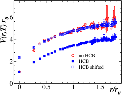
Figure 9: Effect of hypercubic blocking on the potential at $\beta=5.2,\kappa=0.1335$.

In Fig. 9 we compare the static potential from blocked and unblocked configurations. We see that the statistical errors are substantially reduced. Furthermore, rotational invariance is improved, in agreement with earlier observations [24]. The blocking procedure decreases the self energy of the static sources, which causes a constant shift in the potential. In Fig. 9 we shift the potential by $1.33/r_{0}$, so that it agrees with the unblocked potential at $r=\sqrt{2}a$. We find good agreement at all distances, except perhaps at $r=a$. The shift agrees with the change in the asymptotic value of the potential, $-2T\log\,\langle L\rangle$, which was found to be $1.24(25)/r_{0}$. The discrepancy at $r=a$ can be accounted for by perturbative corrections [46]. All our fits are made for $r/r_{0}\geq 1$ thus this point is always discarded.

4.3 Non-Abelian potential

We first fit the static potential by the two-state ansatz (26). This is done for two different choices of $\alpha$, $\alpha=\pi/12$ and $\alpha=0.33$. Examples of the fit for $T/T_{c}=0.87$ and $0.98$ and the second choice $\alpha=0.33$ are shown in Fig. 10. The curves for $\alpha=\pi/12$ and $\alpha=0.33$ are practically indistinguishable from each other, visually and in terms of $\chi^{2}/{\rm dof}$. We also show the asymptotic value of the potential, $-2T\ln\langle L\rangle$. The potential converges to this value at large distances. The two-state ansatz describes the data very well. The fit parameters are given in Tables 7 and 8, where $\sigma(0)=(1.14/r_{0})^{2}$ [3] was used.

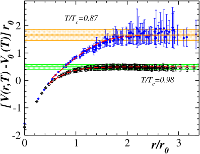
Figure 10: The heavy quark potential at $\beta=5.2$ for $T/T_{c}=0.87$ and $0.98$, together with the fit using $\alpha=0.33$. The horizontal lines show the asymptotic value of the potential, where the shaded area indicates the error.

$\alpha=0.33$
$T/T_{c}$	$V_{0}r_{0}$	$\sigma(T)/\sigma(0)$	$m(T)r_{0}$
0.80	2.33(2)	0.86(3)	1.02(10)
0.87	2.59(3)	0.76(4)	0.89(10)
0.94	2.80(3)	0.79(5)	0.70(8)
0.98	2.85(8)	0.90(12)	0.25(6)
$\alpha=\pi/12$
0.80	2.00(2)	0.97(3)	1.19(11)
0.87	2.23(3)	0.89(4)	1.00(10)
0.94	2.42(4)	0.95(5)	0.90(8)
0.98	2.46(10)	1.05(14)	0.44(7)
Monopole part
0.80	0.47(1)	0.90(1)	1.24(4)
0.87	0.53(1)	0.85(1)	1.07(2)
0.94	0.61(1)	0.84(1)	1.03(3)
0.98	1.06(1)	0.46(1)	0.21(1)

Table 7: Fit parameters of the two-state ansatz (26) at $\beta=5.2$, where we have assumed $\sigma(0)=(1.14/r_{0})^{2}$.

$\alpha=0.33$
$T/T_{c}$	$V_{0}r_{0}$	$\sigma(T)/\sigma(0)$	$m(T)r_{0}$
0.86	2.71(3)	0.74(5)	0.81(7)
0.92	2.87(7)	0.70(10)	0.37(7)
0.96	3.00(6)	0.67(9)	0.25(7)
0.97	3.12(7)	0.57(10)	0.15(7)
0.99	3.16(5)	0.55(8)	0.28(7)
$\alpha=\pi/12$
0.86	2.34(3)	0.88(5)	1.00(6)
0.92	2.49(7)	0.86(10)	0.57(7)
0.96	2.61(6)	0.83(10)	0.45(7)
0.97	2.71(6)	0.73(9)	0.35(6)
0.99	2.75(5)	0.72(8)	0.48(7)
Monopole part
0.86	0.56(2)	0.80(3)	1.18(8)
0.92	0.57(1)	0.80(2)	0.54(2)
0.96	0.64(1)	0.78(2)	0.33(1)
0.97	0.66(1)	0.79(1)	0.27(1)
0.99	0.65(1)	0.79(1)	0.39(1)

Table 8: Fit parameters of the two-state ansatz (26) at $\beta=5.25$, where we have assumed $\sigma(0)=(1.14/r_{0})^{2}$.

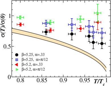
Figure 11: The string tension from a fit of the two-state ansatz (26) as a function of temperature. The quenched value of the string tension [47] is shown for comparison. The shaded region indicate the error bar.

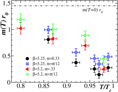
Figure 12: The constituent quark mass from a fit of the two-state ansatz (26) as a function of temperature. The dash–dotted line indicate the zero–temperature quenched value of the mass.

The string tension $\sigma(T)$ and the constituent quark mass $m(T)$ are plotted in Figs. 11 and 12, respectively. In Fig. 11 the quenched value of $\sigma(T)/\sigma(0)$ [47] is shown for comparison. Both the string tension and the constituent quark mass decrease with increasing temperature, as we expect. The results differ by approximately one $\sigma$ between $\alpha=0.33$ and $\alpha=\pi/12$. For lower temperatures, at $T/T_{c}=0.80$ and $T/T_{c}=0.87$, we find rather good agreement between the results of the quenched theory and our results obtained with the choice $\alpha=0.33$. For higher temperatures agreement is much worse, especially for the lighter quark mass. A reason for this discrepancy might be that our Ansatz is not valid at temperatures close to the transition.

Our values for the constituent quark mass $m(T)$ are larger by about $100$ MeV than those reported in [36]. However, one should note a difference between our definition of the self energy and the definition used in Ref. [36].

We are now able to compute the string breaking distance $r_{sb}$ from

$$V_{\rm string}(r_{sb},T)=2m(T)\,.$$ (33)

In Figs. 13 and 14 we show the two energy levels together with the data. The string breaks where the two levels cross.

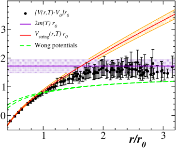
Figure 13: The string potential and the constituent mass as a function of distance at $\beta=5.2$ for $\kappa=0.1335$ ($T/T_{c}=0.87$). The shaded regions indicate the errors.

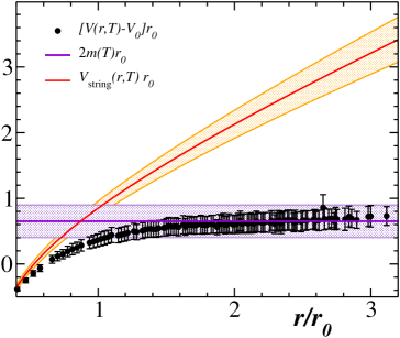
Figure 14: The same as in Fig. 13 but for $\kappa=0.1343$ ($T/T_{c}=0.98$).

The dependence of $r_{sb}$ on the temperature is shown in Fig. 15. We see that $r_{sb}$ decreases as the temperature is increased. The difference of $r_{sb}$ between the two choices of $\alpha$ lies within the error bars.

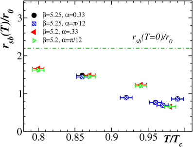
Figure 15: The string breaking distance $r_{sb}$ as a function of temperature. The dash–dotted line indicate the corresponding zero–temperature quenched value.

Let us now consider the screening potential (30). Fitting this potential to our data gives a comparable value of $\chi^{2}/{\rm dof}$. However, the parameters of the fit turn out to be unphysical. For example, at $T/T_{c}=0.80$, $0.87$ and $0.94$ we obtain $\tilde{\sigma}/\sigma(0)=21(6)$, $13(2)$ and $5.5(6)$, respectively. Only close to the deconfinement transition we do find a reasonable value for the string tension: $\tilde{\sigma}/\sigma(0)=0.4(3)$ at $T/T_{c}=0.98$.

The screening potential (30) may be rewritten (up to a constant) in the following form [45]:

$$V^{\rm Wong}(r,T)=\left[-\frac{4}{3}\frac{\alpha_{s}}{r}-\frac{b(T)}{\mu_{0}}\right]e^{-\mu_{0}r}\,.$$ (34)

Taking (as in [45]) $b(T)=b_{0}\left(1-(T/T_{c})^{2}\right)$, $b_{0}=0.35$ GeV$\,{}^{2}$, $\mu_{0}=0.28$ GeV, and $\alpha_{s}\sim 0.32$ ($\alpha_{s}\sim 0.24$) for the charmonium (bottonium) potential, and shifting the potential by a constant so that it agrees with the lattice potential at $r=r_{0}$, we find no agreement between this potential and the lattice data. Thus, the quarkonium spectra derived from this potential [45] need to be revised.

4.4 Monopole part of the potential

We carried out a similar analysis as before for the monopole part of the heavy quark potential, which is obtained from the correlator (31). The fit parameters are given in Tables 7 and 8, and the potential is shown in Fig. 16. The errors are smaller than in the previous fits, as expected. The monopole part of the potential shows no Coulomb term, while at large distances it converges to its asymptotic value $-2T\ln\langle L_{\mathrm{mon}}\rangle$.

Figure 16: The monopole part of the potential as a function of distance at $\beta=5.2$ for $T/T_{c}=0.87$ and $0.98$, together with a fit of the form (32) (dashed curve). The horizontal lines show the asymptotic value of the potential, where the shaded area indicates the error.

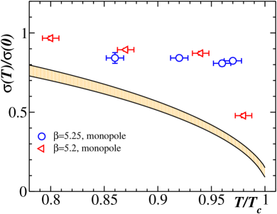
Figure 17: The string tension of the monopole part of the potential as a function of temperature. In the left figure the quenched value of the string tension [47] is shown for comparison. The shaded region indicate the error bar.

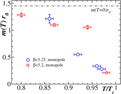
Figure 18: The same as in Fig. 17 but for the constituent quark mass. The dash–dotted line indicate the zero–temperature quenched value of the mass.

The string tension $\sigma_{\rm mon}(T)$ and the constituent quark mass $m_{\rm mon}(T)$ are shown in Fig. 17 and 18, respectively. Because the Coulomb term is absent, we now can determine the string tension much more accurately. We find substantially larger values than in the quenched case. Furthermore, the string tension appears to decrease more slowly as the the system is heated. The constituent quark mass $m_{\rm mon}(T)$ looks very much the same as in the non-Abelian case. The same holds for the string breaking distance, $r^{\rm mon}_{sb}$, which is shown in Fig. 19.

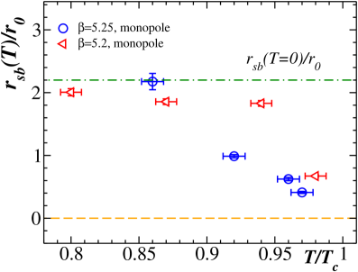
Figure 19: The string breaking distance $r^{\rm mon}_{sb}$ obtained from the monopole potential as a function of temperature. The dash–dotted line indicate the corresponding zero–temperature quenched value.

To shed further light on the string breaking mechanism, we have computed the action density, the color electric field and the monopole current in the vicinity of the (broken) string.

The definitions of observables are the same as in Ref. [12]. We are interested in local Abelian operators of the form:

$${\cal O}(s)=\mbox{diag}({\cal O}_{1}(s),{\cal O}_{2}(s),{\cal O}_{3}(s))\in U(1)\times U(1)\,.$$ (35)

The correlator of the action density – which is $C$-parity even operator – with the product of the monopole Polyakov loops, ${\cal L}_{\rm mon}(\vec{s^{\prime}}){\cal L}_{\rm mon}^{\dagger}(\vec{s}\,^{\prime\prime})$, can be written analogously to Ref. [48]:

$$\langle{\cal O}(s)\rangle_{{\cal L}_{\rm mon}}\equiv\frac{1}{3}\frac{\langle\mbox{Tr}\,{{\cal O}}(s)\mbox{Tr}\,[{\cal L}_{\rm mon}(\vec{s^{\prime}}){\cal L}_{\rm mon}^{\dagger}(\vec{s}\,^{\prime\prime})]\rangle}{\langle\mbox{Tr}\,[{\cal L}_{\rm mon}(\vec{s^{\prime}}){\cal L}_{\rm mon}^{\dagger}(\vec{s}\,^{\prime\prime})]\rangle}-\frac{1}{3}\langle\mbox{Tr}{\mathcal{O}}\rangle\,,$$ (36)

where

$${\cal L}_{\rm mon}(s)=\mbox{diag}(L^{\rm mon}_{1}(s),L^{\rm mon}_{2}(s),L^{\rm mon}_{3}(s))\,,$$ (37)

($cf.$, Eq. (14)).

As for the $C$-parity odd operators ${\cal O}$, such as the color electric field and the monopole current, we have

$$\langle{\cal O}(s)\rangle_{{\cal L}_{\rm mon}}\equiv\frac{\langle\mbox{Tr}\,({{\cal O}}(s)\,[{\cal L}_{\rm mon}(\vec{s^{\prime}}){\cal L}_{\rm mon}^{\dagger}(\vec{s}\,^{\prime\prime})])\rangle}{\langle\mbox{Tr}\,[{\cal L}_{\rm mon}(\vec{s^{\prime}}){\cal L}_{\rm mon}^{\dagger}(\vec{s}\,^{\prime\prime})]\rangle}\,,$$ (38)

in analogy to the case of $SU(2)$ and $U(1)$ theories, Refs. [49].

The monopole part of the action density $\rho_{A}^{{\cal L}_{\rm mon}}$, the monopole part of the color electric field $E_{i}^{{\cal L}_{\rm mon}}$ and the monopole current $k^{{\cal L}_{\rm mon}}$, induced by the Polyakov loops, are then given by

$$\rho_{A}^{{\cal L}_{\rm mon}}(s)=\frac{\beta}{3}\sum_{\mu>\nu}\langle\mbox{diag}(\cos(\theta_{1}^{\rm mon}(s,\mu,\nu)),\cos(\theta_{2}^{\rm mon}(s,\mu,\nu)),\cos(\theta_{3}^{\rm mon}(s,\mu,\nu)))\rangle_{{\cal L}_{\rm mon}}\,,$$ (39)

where the plaquette angles, $\theta^{\rm mon}_{i}(s,\mu,\nu)$, are constructed from the monopole link angles (12),

$$E_{j}^{{\cal L}_{\rm mon}}(s)={\rm i}\,\langle\mbox{diag}(\theta_{1}^{\rm mon}(s,4,j),\theta_{2}^{\rm mon}(s,4,j),\theta_{3}^{\rm mon}(s,4,j))\rangle_{{\cal L}_{\rm mon}}\,,$$ (40)

and

$$k^{\cal L}(^{*}s,\mu)=2\pi{\rm i}\,\langle\mbox{diag}(k_{1}(^{*}s,\mu),k_{2}(^{*}s,\mu),k_{3}(^{*}s,\mu))\rangle_{{\cal L}_{\rm mon}}\,,$$ (41)

respectively.

In Fig. 20 we show the result for $T/T_{c}=0.98$ and three different separations, $r=0.5$, 0.8 and 1.3 fm. Our estimate of the string breaking distance at this temperature is $\approx 0.5$ fm. The figure suggest that the flux tube has disappeared at the latest at $r=1.3$ fm.

(a)                                    (b)                                    (c)

Figure 20: The monopole part of the action density (a), the monopole part of the color electric field (b) and the solenoidal monopole current in the plane perpendicular to the flux tube (c) at $T/T_{c}=0.98$ and distances (from top to bottom) 0.5, 0.8 and 1.3 fm.

5 Monopole density

Another characteristic quantity of the confining vacuum is the monopole density, which we define as

$$\rho=\frac{1}{12N_{t}N_{s}^{3}}\Bigl{\langle}\sum_{i=1}^{3}\sum_{s,\mu}|k_{i}(^{*}s,\mu)|\Bigr{\rangle}\,,$$ (42)

where the monopole current, $k_{i}(^{*}s,\mu)$, is given in (9).

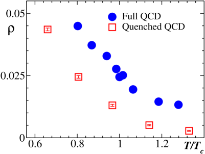
Figure 21: The monopole density at $\beta=5.2$ as a function of temperature.

In Fig. 21 we compare the monopole density of this work with that of the quenched theory. The quenched result has been obtained on the same sized lattice at $\beta=5.8$, 5.9, 6.0, 6.1 and 6.2. The density in full QCD is substantially higher than in the quenched theory, in agreement with our earlier result at $T=0$ [12]. We believe that the introduction of dynamical fermions causes an attraction between monopoles and antimonopoles, which naturally leads to an increase in the monopole density. A similar mechanism has been observed in the case of instantons and antiinstantons [50]. Both mechanisms are, of course, related, because (anti-)instantons are intimately connected with monopoles [51].

Near the finite temperature transition we expect the monopoles to gradually become static as the temperature becomes high. This can be monitored by the asymmetry of the density of spatial and temporal monopole currents [26, 52]:

$$\eta=\frac{\rho_{t}-\rho_{s}}{\rho_{t}+\rho_{s}}\,,$$ (43)

where $\rho_{t}$($\rho_{s}$) is the density of the temporal (spatial) monopole currents,

$$\rho_{t}=\frac{1}{3N_{t}N_{s}^{3}}\Bigr{\langle}\sum_{i=1}^{3}\sum_{s}|k_{i}(^{*}s,4)|\Bigr{\rangle}\,,\quad\rho_{s}=\frac{1}{9N_{t}N_{s}^{3}}\Bigr{\langle}\sum_{i=1}^{3}\sum_{s}\sum^{3}_{\mu=1}|k_{i}(^{*}s,\mu)|\Bigr{\rangle}\,.$$ (44)

If all currents are time-like, then this quantity is unity, while in the case of an isotropic distribution it is zero.

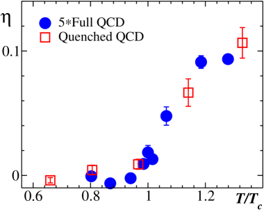
Figure 22: The asymmetry of the monopole density at $\beta=5.2$ as a function of temperature.

In Fig. 22 we plot the asymmetry $\eta$ as a function of temperature. We compare the result with the predictions of the quenched theory. It is found that $\eta$ is zero in the confined phase and nonzero in the deconfined phase. In the deconfinement phase the value of $\eta$ is about 5 times smaller in full QCD compared to the quenched theory. A reason for this may be rooted in a different nature of the transition which is of the first order phase in the quenched case while in full QCD one observes a smooth crossover.

6 Conclusions

We have studied QCD with two flavors of dynamical quarks at finite temperature on a $16^{3}\,8$ lattice. At the phase transition the lattice spacing is $a\approx 0.12$ fm. We employed non-perturbatively improved Wilson fermions, so that we may expect finite cut-off effects to be small.

To determine the parameters of the transition, notably the transition temperature and the string tension, and to shed light on the dynamics of the transition, it helped to resort to Abelian variables in the maximally Abelian gauge.

We observed string breaking in Polyakov loop correlators. This is a level crossing phenomenon. Accordingly, we fitted the correlator by a two-state ansatz, consisting of a string state and a two-meson state. We found good agreement of this ansatz with our numerical data for $T\lesssim T_{c}$, while we could rule out previously proposed single-state correlation functions. The string breaking distance was found to be $r_{\rm sb}\approx 1$ fm at $T/T_{c}\approx 0.8$, our lowest temperature. String breaking is also clearly visible in the action density, the color electric field distribution and the solenoidal monopole current around the static sources.

To make contact with the chiral limit, we need to increase $N_{t}$, because the coupling cannot be taken smaller than $\beta\approx 5.2$. Work on $24^{3}\,10$ lattices at $m_{\pi}/m_{\rho}\approx 0.6$ is in progress. Preliminary results have been presented in [53].