BI-TP 2003/38
Remarks on the multi-parameter reweighting method for the study of lattice QCD at non-zero temperature and density

Abstract

We comment on the reweighting method for the study of finite density lattice QCD. We discuss the applicable parameter range of the reweighting method for models which have more than one simulation parameter. The applicability range is determined by the fluctuations of the modification factor of the Boltzmann weight. In some models having a first order phase transition, the fluctuations are minimized along the phase transition line if we assume that the pressure in the hot and the cold phase is balanced at the first order phase transition point. This suggests that the reweighting method with two parameters is applicable in a wide range for the purpose of tracing out the phase transition line in the parameter space. To confirm the usefulness of the reweighting method for 2 flavor QCD, the fluctuations of the reweighting factor are measured by numerical simulations for the cases of reweighting in the quark mass and chemical potential directions. The relation with the phase transition line is discussed. Moreover, the sign problem caused by the complex phase fluctuations is studied.

I Introduction

The study of the phase structure of QCD at non-zero temperature $T$ and non-zero quark chemical potential $\mu_{q}$ is currently one of the most attractive topics in particle physics [1, 2]. The heavy-ion collision experiments aiming to produce the quark-gluon plasma (QGP) are running at BNL and CERN, for which the interesting regime is rather low density. Moreover a new color superconductor phase is expected in the region of low temperature and high density. In the last few years, remarkable progress has been achieved in the numerical study by Monte-Carlo simulations of lattice QCD at low density. It was shown that the phase transition line, separating hadron phase and QGP phase, can be traced out from $\mu_{q}=0$ to finite $\mu_{q}$, and it was also possible to investigate the equation of state quantitatively at low density. The main difficulty of the study at non-zero baryon density is that the Monte-Carlo method is not applicable directly at finite density, since the fermion determinant is complex for non-zero $\mu_{q}$ and configurations cannot be generated with the probability of the Boltzmann weight. The most popular technique to study at non-zero $\mu_{q}$ is the reweighting method; performing simulations at ${\rm Re}(\mu_{q})=0$, and then modify the Boltzmann weight at the step of measurement of observables [3, 4, 5, 6]. The Glasgow method [7] is one of the reweighting methods. A composite (Glasgow) reweighting method has recently been proposed by [8]. Another approach is analytic continuation from simulations at imaginary chemical potential [9, 10, 11]. Moreover, calculating coefficients of a Taylor expansion in terms of $\mu_{q}$ is also a hopeful approach for the study at non-zero baryon density [4, 12, 13, 14]. The studies by Taylor expansion or imaginary chemical potential require analyticity of physical quantities as functions of $T$ and $\mu_{q}$, while the reweighting method has a famous “sign problem”. The sign problem is caused by complex phase fluctuations of the fermion determinant, which are measured explicitly in Ref. [15], and also Ref. [16] is a trial to avoid the sign problem.

In this paper, we make comments on the reweighting method with respect to more than one simulation parameter, particularly, including a chemical potential. Because the fluctuation of the modification factor (reweighting factor) enlarges the statistical error, the applicable range of this method is determined by the fluctuation of the reweighting factor. When the error becomes considerable in comparison with the expectation value, the reweighting method breaks down. An interesting possibility is given in the following case: when we change two parameters at the same time, the reweighting factors for two parameters might cancel each other, then the error does not increase and also the expectation values of physical quantities do not change by this parameter shift. Therefore finding such a direction provides useful information for mapping out the value of physical quantities in the parameter space. As we will see below, there is such a direction in the parameter space and the knowledge of this property of the reweighting method makes the method more useful. Fodor and Katz [3] investigated the phase transition line for rather large $\mu_{q}$. This argument may explain why they could calculate $\beta_{c}$ for such large $\mu_{q}$.

In the next section, we explain the reweighting method with multi-parameters. Then, in Sec. III, the case of SU(3) pure gauge theory on an anisotropic lattice is considered as the simplest example, and we proceed to full QCD with a first order phase transition in Sec. IV. For 2-flavor QCD, the reweighting method with respect to quark mass is discussed in Sec. V. The application to non-zero baryon density is discussed in Sec. VI. The problem of the complex measure is also considered in Sec. VII. Conclusions are given in Sec. VIII.

II Reweighting method and the applicability range

The reweighting method is based on the following identity:

$$\langle{\cal O}\rangle_{(\beta,m,\mu)} = \frac{1}{{\cal Z}_{(\beta,m,\mu)}}\int DU{\cal O}(\det M(m,\mu))^{N_{\rm f}}e^{-S_{g}(\beta)}$$ (1)

$$= \frac{\left\langle{\cal O}e^{F}e^{G}\right\rangle_{(\beta_{0},m_{0},\mu_{0})}}{\left\langle e^{F}e^{G}\right\rangle_{(\beta_{0},m_{0},\mu_{0})}}=\frac{\left\langle{\cal O}e^{\Delta F}e^{\Delta G}\right\rangle_{(\beta_{0},m_{0},\mu_{0})}}{\left\langle e^{\Delta F}e^{\Delta G}\right\rangle_{(\beta_{0},m_{0},\mu_{0})}}.$$ (2)

Here $M$ is the quark matrix, $S_{g}$ is the gauge action, $N_{\rm f}$ is the number of flavors ($N_{\rm f}/4$ for staggered type fermions instead of $N_{\rm f}$), $F=N_{\rm f}[\ln\det M(m,\mu)-\ln\det M(m_{0},\mu_{0})],$ $G=(\beta-\beta_{0})P,P=-\partial S_{g}/\partial\beta,$ $\beta=6/g^{2},$ and $\Delta F[G]=F[G]-\langle F[G]\rangle$. $m$ and $\mu\equiv\mu_{q}a$ are the bare quark mass and chemical potential in a lattice unit, respectively. The expectation value $\langle{\cal O}\rangle_{(\beta,m,\mu)}$ can, in principle, be computed by simulation at $(\beta_{0},m_{0},\mu_{0})$ using this identity [17]. However, a problem of the reweighting method is that the fluctuation of $e^{\Delta F}e^{\Delta G}=e^{F}e^{G}/(e^{\langle F\rangle}e^{\langle G\rangle})$ enlarges the statistical error of the numerator and denominator of Eq.(2). The worst case, which is called “Sign problem”, is that the sign of the reweighting factor changes frequently during Monte-Carlo steps, then the expectation values in Eq.(2) become vanishingly small in comparison with the error, and this method does not work. However, the fluctuations cause the $\beta$, $m$ and $\mu$ dependence of $\langle{\cal O}\rangle_{(\beta,m,\mu)}$. Otherwise, if $e^{F}e^{G}$ does not fluctuate, $e^{\Delta F}e^{\Delta G}=1$ and $\langle{\cal O}\rangle_{(\beta,m,\mu)}$ does not change with parameter change. Roughly speaking, the difference of $\langle{\cal O}\rangle_{(\beta,m,\mu)}$ from $\langle{\cal O}\rangle_{(\beta_{0},m_{0},\mu_{0})}$ increases as the magnitude of fluctuations of $F$ and $G$ increases and, if $F$ and $G$ have a correlation, the increase of the total fluctuation as a function of $\beta$, $m$ and $\mu$ is non-trivial. Therefore, it is important to discuss the correlation between $e^{F}$ and $e^{G}$ and to estimate the total fluctuation of the reweighting factor in the parameter space in order to estimate the applicability range of the reweighting method in the parameter space and how the system changes by parameter shifts. This is helpful information for the study of QCD thermodynamics.

III SU(3) gauge theory on an anisotropic lattice

Let us start with the case of SU(3) pure gauge theory on an anisotropic lattice, having two different lattice spacings for space and time directions: $a_{\sigma}$ and $a_{\tau}$. As we will show for this case, there is a clear relation between the phase transition line and the direction which minimizes the fluctuation of the reweighting factor. The action is

$$S_{g}=-\beta_{\sigma}\sum_{x}P_{\sigma}(x)-\beta_{\tau}\sum_{x}P_{\tau}(x),$$ (3)

where $P_{\sigma(\tau)}$ is spatial (temporal) plaquette. The SU(3) pure gauge theory has a first order phase transition. At the transition point $(T_{c})$, there exist two phases simultaneously. For the two phases to coexist, the pressure in these phases must be equal: $\Delta p\equiv p^{\rm(hot)}-p^{\rm(cold)}=0$. If we require $\Delta p=0$, we find that the phase transition line in the parameter space of $(\beta_{\sigma},\beta_{\tau})$ has to run in such a direction that the fluctuation of the reweighting factor is minimized when we perform a simulation on the phase transition point and apply the reweighting in the $(\beta_{\sigma},\beta_{\tau})$ plane.

A significant feature of a Monte-Carlo simulation at a first order phase transition point is the occurrence of flip-flops between configurations of hot and cold phases. If one write a histogram of the action density, i.e. the plaquette: $P_{\sigma}$ and $P_{\tau}$, there exist two peaks. The value of the action density changes sometimes from one near one peak to one near the other peak during Monte-Carlo steps [18, 19]. The flip-flop is the most important fluctuation; in fact, the flip-flop makes the strong peak of susceptibilities of observables such as the plaquette or the Polyakov loop at the transition point. Also, the flip-flop implies strong correlations between $P_{\sigma}$ and $P_{\tau}$ because the values of $P_{\sigma}$ and $P_{\tau}$ change simultaneously between the typical values of the two phases in the $(P_{\sigma},P_{\tau})$ plane.

Here, we discuss the fluctuation of the reweighting factor when one performs a simulation at the transition point, $(\beta_{\sigma 0},\beta_{\tau 0})$. An expectation value of ${\cal O}$ at $(\beta_{\sigma},\beta_{\tau})$ on an anisotropic lattice is calculated by

$$\langle{\cal O}\rangle_{(\beta_{\sigma},\beta_{\tau})}=\left.\left\langle{\cal O}e^{-\Delta S_{g}}\right\rangle_{(\beta_{\sigma 0},\beta_{\tau 0})}\right/\left\langle e^{-\Delta S_{g}}\right\rangle_{(\beta_{\sigma 0},\beta_{\tau 0})},$$ (4)

where $\Delta S_{g}=-\Delta\beta_{\sigma}\sum_{x}P_{\sigma}(x)-\Delta\beta_{\tau}\sum_{x}P_{\tau}(x),$ and $\Delta\beta_{\sigma(\tau)}=\beta_{\sigma(\tau)}-\beta_{\sigma(\tau)0}.$ For simplification, we ignore the local fluctuation around the two peaks of the histogram of the action density and consider only the flip-flop between hot and cold phases, since it is the most important fluctuation at the first order phase transition point. Then, the fluctuation is estimated by the difference of the reweighting factor between hot and cold phases, up to first order,

$$|e^{-\Delta S_{g}^{\rm(hot)}}-e^{-\Delta S_{g}^{\rm(cold)}}|\approx 3N_{\rm site}|\Delta\beta_{\sigma}(\bar{P}_{\sigma}^{\rm(hot)}-\bar{P}_{\sigma}^{\rm(cold)})+\Delta\beta_{\tau}(\bar{P}_{\tau}^{\rm(hot)}-\bar{P}_{\tau}^{\rm(cold)})|+\cdots,$$ (5)

where $\bar{P}_{\sigma}^{\rm hot(cold)}$ and $\bar{P}_{\tau}^{\rm hot(cold)}$ are the average values of the spatial and temporal plaquettes for configurations in the hot (cold) phase and $N_{\rm site}\equiv N_{\sigma}^{3}\times N_{\tau}$ is the number of sites for an $N_{\sigma}^{3}\times N_{\tau}$ lattice. Hence, along the line which has a slope

$$\frac{{\rm d}\beta_{\sigma}}{{\rm d}\beta_{\tau}}=-\frac{\bar{P}_{\tau}^{\rm(hot)}-\bar{P}_{\tau}^{\rm(cold)}}{\bar{P}_{\sigma}^{\rm(hot)}-\bar{P}_{\sigma}^{\rm(cold)}},$$ (6)

the fluctuation of the reweighting factor is canceled to leading order.

On the other hand, since $V=(N_{\sigma}a_{\sigma})^{3}$ and $T=(N_{\tau}a_{\tau})^{-1}$, pressure is defined by

$$p = T\left.\frac{\partial\ln{\cal Z}}{\partial V}\right|_{T}=\frac{1}{3N_{\sigma}^{3}N_{\tau}a_{\sigma}^{2}a_{\tau}}\left.\frac{\partial\ln{\cal Z}}{\partial a_{\sigma}}\right|_{a_{\tau}},$$ (7)

$$\frac{p}{T^{4}} = N_{\tau}^{4}\left(\frac{a_{\tau}}{a_{\sigma}}\right)^{3}\left[a_{\sigma}\frac{\partial\beta_{\sigma}}{\partial a_{\sigma}}(\langle\bar{P}_{\sigma}\rangle-\langle\bar{P}_{\sigma}\rangle_{0})+a_{\sigma}\frac{\partial\beta_{\tau}}{\partial a_{\sigma}}(\langle\bar{P}_{\tau}\rangle-\langle\bar{P}_{\tau}\rangle_{0})\right],$$ (8)

where $\bar{P}_{\sigma(\tau)}=(3N_{\rm site})^{-1}\sum_{x}P_{\sigma(\tau)}(x)$, and $\langle\bar{P}_{\sigma(\tau)}\rangle_{0}$ is the expectation value of the plaquette on a $T=0$ lattice for the normarization.

By separating the configurations into those in hot and cold phases [18, 19], the gap of pressure between hot and cold phases at $T_{c}$ is computed by

$$\Delta\frac{p}{T^{4}} \equiv \frac{p^{\rm(hot)}}{T^{4}}-\frac{p^{\rm(cold)}}{T^{4}}$$ (9)

$$= N_{\tau}^{4}\left(\frac{a_{\tau}}{a_{\sigma}}\right)^{3}\left[a_{\sigma}\frac{\partial\beta_{\sigma}}{\partial a_{\sigma}}(\bar{P}_{\sigma}^{\rm(hot)}-\bar{P}_{\sigma}^{\rm(cold)})+a_{\sigma}\frac{\partial\beta_{\tau}}{\partial a_{\sigma}}(\bar{P}_{\tau}^{\rm(hot)}-\bar{P}_{\tau}^{\rm(cold)})\right].$$ (10)

Since the gap of pressure should vanish, $\Delta p=0$,

$$\left.\frac{\partial\beta_{\sigma}}{\partial a_{\sigma}}\right/\frac{\partial\beta_{\tau}}{\partial a_{\sigma}}=-\frac{\bar{P}_{\tau}^{\rm(hot)}-\bar{P}_{\tau}^{\rm(cold)}}{\bar{P}_{\sigma}^{\rm(hot)}-\bar{P}_{\sigma}^{\rm(cold)}}.$$ (11)

Moreover, because $T_{c}=(N_{\tau}a_{\tau})^{-1}$ on the phase transition line, $a_{\tau}$ keeps constant with $(N_{\tau}T_{c})^{-1}$ along the transition line, i.e.

$$\Delta a_{\tau}=\frac{\partial a_{\tau}}{\partial\beta_{\sigma}}\Delta\beta_{\sigma}+\frac{\partial a_{\tau}}{\partial\beta_{\tau}}\Delta\beta_{\tau}=0,$$ (12)

when one changes parameters $(\beta_{\sigma},\beta_{\tau})\to(\beta_{\sigma}+\Delta\beta_{\sigma},\beta_{\tau}+\Delta\beta_{\tau})$ along the phase transition line. Then the slope of the phase transition line $(r_{t})$ [20] is obtained by

$$r_{t}\equiv\left.\frac{{\rm d}\beta_{\sigma}}{{\rm d}\beta_{\tau}}\right|_{T_{c}}=\left.-\frac{\partial a_{\tau}}{\partial\beta_{\tau}}\right/\frac{\partial a_{\tau}}{\partial\beta_{\sigma}}=\left.\frac{\partial\beta_{\sigma}}{\partial a_{\sigma}}\right/\frac{\partial\beta_{\tau}}{\partial a_{\sigma}},$$ (13)

where we used an identify:

$$\left(\begin{array}[]{cc}\frac{\partial\beta_{\sigma}}{\partial a_{\sigma}}&\frac{\partial\beta_{\tau}}{\partial a_{\sigma}}\\ \frac{\partial\beta_{\sigma}}{\partial a_{\tau}}&\frac{\partial\beta_{\tau}}{\partial a_{\tau}}\end{array}\right)=\frac{1}{\frac{\partial a_{\tau}}{\partial\beta_{\tau}}\frac{\partial a_{\sigma}}{\partial\beta_{\sigma}}-\frac{\partial a_{\tau}}{\partial\beta_{\sigma}}\frac{\partial a_{\sigma}}{\partial\beta_{\tau}}}\left(\begin{array}[]{cc}\frac{\partial a_{\tau}}{\partial\beta_{\tau}}&-\frac{\partial a_{\tau}}{\partial\beta_{\sigma}}\\ -\frac{\partial a_{\sigma}}{\partial\beta_{\tau}}&\frac{\partial a_{\sigma}}{\partial\beta_{\sigma}}\end{array}\right).$$ (18)

Hence, the condition for $\Delta p=0$ becomes

$$\frac{\bar{P}_{\tau}^{\rm(hot)}-\bar{P}_{\tau}^{\rm(cold)}}{\bar{P}_{\sigma}^{\rm(hot)}-\bar{P}_{\sigma}^{\rm(cold)}}=-r_{t}.$$ (19)

This equation for ${\rm d}\beta_{\sigma}/{\rm d}\beta_{\tau}$ may correspond to the Clausius-Clapeyron equation in the $(p,T)$ plane: ${\rm d}p/{\rm d}T=\Delta S/\Delta V$ ($S$: entropy). In fact, Eq.(19) and the vanishing pressure gap, $\Delta p=0,$ are confirmed by calculating the slope of the transition line from the peak position of the Polyakov loop susceptibility obtained by numerical simulations in Ref. [20]. Historically, the non-zero gap of pressure at the transition point had been a problem for long time. The reason of $\Delta p\neq 0$ was that the precise non-perturbative measurement of the anisotropy coefficients, $a_{\sigma}(\partial\beta_{\sigma}/\partial a_{\sigma}),a_{\sigma}(\partial\beta_{\tau}/\partial a_{\sigma}),$ etc., had been difficult, and the perturbative value [21] cannot be used at the phase transition point for $N_{\tau}=4$ or $6$. After the precise measurement of the anisotropy coefficients became possible, the problem of a non-zero pressure gap was solved. Also, determinations of these coefficients by another non-perturbative method have been done in Refs. [22, 23, 24].

From Eq.(6) and Eq.(19), we find that the direction which minimizes the fluctuation of the reweighting factor must be the same as the direction of the phase transition line in the $(\beta_{\sigma},\beta_{\tau})$ plane, if pressure in hot and cold phases are balanced at $T_{c}$, $\Delta p=0$. Here, in practice, we estimate the fluctuation of $e^{-\Delta S_{g}}$ by a numerical simulation. We compute the standard deviation of the reweighting factor using the data obtained in Ref. [19]. The lattice size is $24^{2}\times 36\times 4$. The data is generated by the standard Wilson gauge action with $\beta_{\sigma}=\beta_{\sigma}=5.6925$, that is just on the transition line, $\beta_{c}=5.69245(23)$ for $N_{\tau}=4$ at $a_{\sigma}=a_{\tau}$. Ellipses in Fig.1 are the contour lines of the standard deviation normalized by the mean value: $\sqrt{\langle(e^{-\Delta S_{g}})^{2}\rangle-\langle e^{-\Delta S_{g}}\rangle^{2}}/\langle e^{-\Delta S_{g}}\rangle,$ and we write this value in Fig. 1. We also denote the phase transition line, obtained by the measurement of the Polyakov loop susceptibility assuming that the peak position of the susceptibility is the phase transition point [20], by a bold line, and dashed lines are the upper bound and lower bound. We find that the phase transition line and the line which minimizes fluctuations are consistent. This result also means that the reweighting method is applicable in a wide range for the determination of the phase transition line in the parameter space of SU(3) gauge theory on an anisotropic lattice, since the increase of the statistical error caused by the reweighting is small along the transition line.

We note that, from Eq.(19), $\Delta S_{g}^{\rm(hot)}$ and $\Delta S_{g}^{\rm(cold)}$ in Eq.(5) are equal under the change along the phase transition line, hence the fluctuations are canceled in every order of $\Delta\beta_{\sigma(\tau)}$. For SU(3) pure gauge theory on an anisotropic lattice, the system is independent of $a_{\sigma}/a_{\tau}$ in a physical unit, hence the system does not change along the transition line except for the volume, $V=(N_{\sigma}a_{\sigma})^{3}$, if $N_{\sigma}$ is finite. Because physical quantities does not change without the fluctuation of reweighting factor, this result is quite natural.

IV Full QCD with a first order phase transition

Next, we extend this discussion for the case of full QCD with a first order phase transition such as 3 flavor QCD near the chiral limit. The reweighting method is applied in the parameter space of $(m,\beta)$. We consider Helmholtz free energy density $f=-T\ln{\cal Z}/V$ for a canonical ensemble which is equal to minus pressure, $p=-f$, for a large homogeneous system. Under a parameter change from $(m,\beta)$ to $(m+\Delta m,\beta+\Delta\beta)$, the variation of the free energy is given, up to the first order, by

$$\left.\frac{f}{T^{4}}\right|_{(m+\Delta m,\beta+\Delta\beta)}-\left.\frac{f}{T^{4}}\right|_{(m,\beta)}=-N_{\tau}^{4}\left[(\langle\bar{Q}_{1}\rangle-\langle\bar{Q}_{1}\rangle_{0})\Delta m+6(\langle\bar{P}\rangle-\langle\bar{P}\rangle_{0})\Delta\beta\right]+\cdots$$ (20)

where $\bar{Q}_{1}=N_{\rm site}^{-1}N_{\rm f}\partial(\ln\det M)/\partial m$ and $\bar{P}=-(6N_{\rm site})^{-1}\partial S_{g}/\partial\beta$. For the normalization at $T=0$, we subtract the zero temperature contribution, $\langle\bar{P}\rangle_{0}$ and $\langle\bar{Q}_{1}\rangle_{0}$. Here, we should notice that the first derivatives of the free energy are discontinuous at the phase transition line, hence we cannot estimate the difference of the free energy beyond the transition line by this equation.

We assume that the gap of the pressure is zero in the entire parameter space $(m,\beta)$. We change $m$ and $\beta$ along the phase transition line starting at two points: just above and just below $\beta_{c}$, without crossing the transition line. Then the change of the free energy must be the same for both these cases, since a pressure gap is not generated under this variation, i.e. $\Delta(\Delta p)=0$. Hence, up to first order of $\Delta m$ and $\Delta\beta$,

$$\left(\left.\frac{f}{T^{4}}\right|_{(m+\Delta m,\beta+\Delta\beta)}^{(\rm hot)}-\left.\frac{f}{T^{4}}\right|_{(m,\beta)}^{(\rm hot)}\right)-\left(\left.\frac{f}{T^{4}}\right|_{(m+\Delta m,\beta+\Delta\beta)}^{(\rm cold)}-\left.\frac{f}{T^{4}}\right|_{(m,\beta)}^{(\rm cold)}\right)$$ (21)

$$=-N_{\tau}^{4}\left[(\bar{Q}_{1}^{\rm(hot)}-\bar{Q}_{1}^{\rm(cold)})\Delta m+6(\bar{P}^{\rm(hot)}-\bar{P}^{\rm(cold)})\Delta\beta\right]+\cdots=0.$$ (22)

is required on the first order phase transition line. From this equation, we obtain a similar relation as Eq.(19):

$$\frac{\bar{Q}_{1}^{\rm(hot)}-\bar{Q}_{1}^{\rm(cold)}}{6(\bar{P}^{\rm(hot)}-\bar{P}^{\rm(cold)})}=-\left.\frac{{\rm d}\beta}{{\rm d}m}\right|_{T_{c}}.$$ (23)

On the other hand, the change of the reweighting factor under flip-flop is

$$|e^{\Delta F^{\rm(hot)}}e^{\Delta G^{\rm(hot)}}-e^{\Delta F^{\rm(cold)}}e^{\Delta G^{\rm(cold)}}|$$ (24)

$$\approx N_{\rm site}\left[(\bar{Q}_{1}^{\rm(hot)}-\bar{Q}_{1}^{\rm(cold)})\Delta m+6(\bar{P}^{\rm(hot)}-\bar{P}^{\rm(cold)})\Delta\beta\right]+\cdots.$$ (25)

If we ignore the local fluctuation around the peaks of the distribution of $P$ and $Q_{1}$, again, the direction for which the fluctuation is canceled is

$$-\frac{{\rm d}\beta}{{\rm d}m}=\frac{\bar{Q}_{1}^{\rm(hot)}-\bar{Q}_{1}^{\rm(cold)}}{6(\bar{P}^{\rm(hot)}-\bar{P}^{\rm(cold)})}$$ (26)

This is the same direction as the phase transition line. Therefore, the fluctuation of the reweighting factor along the phase transition line remains small, i.e. the statistical error does not increase so much.

We obtained the same result as for the pure gauge theory on an anisotropic lattice, and this argument seems to be quite general for models with a first order phase transition, including models with chemical potential. However, there is a difference. Under the change of $a_{\sigma}/a_{\tau}$, any physics does not change along the $T_{c}$ line, but physical quantities, in general, depend on the quark mass. Although the dependence on $m$ might be much smaller than the dependence on $T/T_{c}$, if the fluctuation of the reweighting factor is completely canceled, any $m$-dependence is not obtained. In this discussion, we ignored the local fluctuation around the peaks in the hot and cold phase respectively, but the local fluctuation may play an important role for the $m$-dependence. Also, the sign problem for nonzero baryon density is caused by complex phase fluctuations of the reweighting factor (see Sec. VII.), that is by the local fluctuations. Hence the local fluctuation may, in particular, be important at non-zero baryon density.

V Quark mass reweighting for 2 flavor QCD

As we have seen in the previous two sections, the multi-parameter reweighting seems to be efficient to trace out the phase transition line in a wide range of the parameter space. One of the most interesting applications is finding the (pseudo-) critical line $(\beta_{c})$ in the $(m,\beta)$ plane for 2 flavor or 2+1 flavor QCD. The phase transition for 2 flavor QCD at finite quark mass is expected to be crossover, which is not related to any singularity in thermodynamic observables, and that for 3 flavor QCD is crossover for quark masses larger than a critical quark mass, and is of first order for light quarks. The precise measurement of the (pseudo-) critical line is required for the extrapolation to the physical quark masses and for the study of universality class, e.g. to investigate for the 2 flavor case whether the chiral phase transition at finite temperature is in the same universality class as the 3-dimensional O(4) spin model or not.

In Ref. [4], we applied the reweighting method in the $(m,\beta)$ plane for 2 flavor QCD, and calculated the slope of the transition line, ${\rm d}\beta_{c}/{\rm d}m$, where the reweighting factor with respect to quark mass was expanded into a power series and higher order terms which does not affect the calculation of the slope were neglected. The results for ${\rm d}\beta_{c}/{\rm d}m$ compared well with the data of $\beta_{c}(m)$ obtained by direct calculations, without applying the reweighting method, demonstrating the reliability of a reweighting in a parameter of the fermion action. In this section, we discuss the relation between the fluctuation of the reweighting factor and the phase transition line in the $(m,\beta)$ plane for 2 flavor QCD at finite quark mass, i.e. at the crossover transition, by measuring the fluctuation in numerical simulations.

For the presence of a direction for which the two reweighting factors from the gauge and the fermion action cancel, a correlation between these reweighting factors during Monte-Carlo steps is required. We estimate the correlation between these reweighting factors using the configurations in Ref. [4]. A combination of the Symanzik improved gauge action and 2 flavors of the p-4 improved staggered fermion action is employed [25]. The parameters are $m_{0}=0.1,\beta_{0}=\{3.64,3.645,3.65,3.655,3.66,3.665$ and $3.67\}$. The lattice size is $16^{3}\times 4$. 7800-58000 trajectories are used for measurements at each $\beta$. The details are given in Ref. [4].

In the vicinity of the simulation point, the correlation of the reweighting factors can be approximated by

$$\langle e^{F}e^{G}\rangle-\langle e^{F}\rangle\langle e^{G}\rangle\equiv\langle\Delta e^{F}\Delta e^{G}\rangle\approx\langle\Delta Q_{1}\Delta P\rangle(m-m_{0})(\beta-\beta_{0})+\cdots,$$ (27)

where $P=-\partial S_{g}/\partial\beta$, $F=\sum_{n=1}^{\infty}Q_{n}(m-m_{0})^{n},$ and we denote $\Delta X\equiv X-\langle X\rangle$ for $X=\{P,Q_{n},\cdots\}$. The $Q_{n}$ are obtained by

$$Q_{1}=(N_{\rm f}/4){\rm tr}M^{-1},\ \ Q_{2}=-(N_{\rm f}/8){\rm tr}(M^{-1}M^{-1}),\cdots,$$ (28)

for standard staggered fermions and also for p4-improved staggered fermions. We calculate the value of $\langle\Delta Q_{1}\Delta P\rangle\equiv\langle Q_{1}P\rangle-\langle Q_{1}\rangle\langle P\rangle$. The random noise method is used for the calculation of $Q_{n}$. The results for $\langle\Delta Q_{1}\Delta P\rangle$ are listed in Table I. We find strong correlation between the gauge and fermion parts of the reweighting factor.

Then we compute the total fluctuation of the reweighting factor as a function of $m$ and $\beta$ near the simulation point. Up to second order in $\beta-\beta_{0}$ and $m-m_{0}$, the square of the standard deviation is written as

$$\langle[\Delta(e^{F}e^{G})]^{2}\rangle \approx \langle(\Delta Q_{1})^{2}\rangle(m-m_{0})^{2}+2\langle\Delta Q_{1}\Delta P\rangle(m-m_{0})(\beta-\beta_{0})$$ (30)

$$+\langle(\Delta P)^{2}\rangle(\beta-\beta_{0})^{2}+\cdots.$$

If we approximate in this form, lines of constant fluctuation (standard deviation) in the $(m,\beta)$ plane form ellipses. We also compute $\langle(\Delta Q_{1})^{2}\rangle$ and $\langle(\Delta P)^{2}\rangle$, which are written in Table I. The values at $\beta_{c}=3.6492(22)$ are interpolated by applying the reweighting method for $\beta$ direction combining the data at seven simulation points [17]. The lines of constant fluctuation are drown in Fig. 2. Numbers in this figure are the squares of the standard deviation divided by $N_{\rm site}$. It is found that these ellipses spread over one direction and the increase of the fluctuation is small along the direction. We also show the slope of the phase transition line by two lines: upper bound and lower bound of the derivative of $\beta_{c}$ with respect to $m$ obtained by measuring the peak position of the chiral susceptibility, ${\rm d}\beta_{c}/{\rm d}m=1.05(14)$ for $m_{0}=0.1$ [4]. We see that the directions of small fluctuations and of the phase transition are roughly the same. Since the fluctuation enlarges the statistical error of an observable, this figure can be also regarded as a map indicating the increase of the statistical error due to the reweighting. Therefore, we understand that the reweighting method can be applied in a wide range of parameters along the phase transition line if one performs simulations at the phase transition point.

Moreover, it might be also important that these two directions are not exactly the same because, if the fluctuation is completely canceled along the transition line, no quantity can change, but the system should change as a function of quark mass even on the transition line, e.g. the chiral susceptibility should become larger as $m$ decreases.

VI Chemical potential reweighting for 2-flavor QCD

A Correlation among the reweighting factors

Next, let us discuss the reweighting method for non-vanishing chemical potential. The reweighting method is really important for the study of finite density QCD since direct simulations are not possible for non-zero baryon density at present. However, the complex measure problem (sign problem) is known to be a difficult problem. The reweighting factor for non-zero $\mu$ is complex. If the complex phase fluctuates rapidly and the reweighting factor changes sign frequently, the expectation values in Eq.(2) become smaller than the error. Then the reweighting method breaks down. Therefore it is important to investigate the reweighting factor, including the complex phase, in practical simulations.

First of all, we separate the fermion reweighting factor $e^{F}$ into an amplitude $|e^{F}|$ and a phase factor $e^{i\theta}$, and investigate the correlation among $|e^{F}|$, $e^{i\theta}$ and the gauge part $e^{G}$, where $e^{G}$ is real. As is shown in Ref. [4], the phase factor and the amplitude can be written as the odd and even terms of the Taylor expansion of $\ln\det M$, respectively, since the odd terms are purely imaginary and the even terms are real at $\mu=0$. Denoting $F=\sum_{n=1}^{\infty}R_{n}\mu^{n},$

$$|e^{F}|=\exp\{\sum_{n=1}^{\infty}{\rm Re}(R_{2n})\mu^{2n}\}\ \ {\rm and}\ \ e^{i\theta}=\exp\{i\sum_{n=1}^{\infty}{\rm Im}(R_{2n-1})\mu^{2n-1}\}.$$ (31)

We study the correlation among these factors in the vicinity of the simulation point $(\beta_{0},\mu_{0}=0)$. Up to $O(\beta-\beta_{0},\mu^{2})$, the reweighting factor is

$$e^{i\theta}|e^{F}|e^{G}\approx 1+R_{1}\mu+(R_{1}^{2}/2)\mu^{2}+R_{2}\mu^{2}+P(\beta-\beta_{0})+\cdots.$$ (32)

We compute the correlations, $\langle\Delta(R_{1}^{2}/2)\Delta P\rangle,$ $\langle\Delta R_{2}\Delta P\rangle,$ and $\langle\Delta(R_{1}^{2}/2)\Delta R_{2}\rangle$ at $\mu=0$, which correspond to the correlations of $(e^{i\theta},e^{G})$, $(|e^{F}|,e^{G})$ and $(e^{i\theta},|e^{F}|)$, respectively. $\Delta X\equiv X-\langle X\rangle$ for $X=\{P,R_{n},\cdots\}$. Here, $\langle\Delta R_{1}\Delta P\rangle$ and $\langle\Delta R_{1}\Delta R_{2}\rangle$ are zero at $\mu=0$ because $R_{1}$ is purely imaginary. The $R_{n}$ are obtained by

$$R_{1} = \frac{N_{\rm f}}{4}\frac{\partial\ln\det M}{\partial\mu}=\frac{N_{\rm f}}{4}{\rm tr}\left(M^{-1}\frac{\partial M}{\partial\mu}\right),$$ (33)

$$R_{2} = \frac{N_{\rm f}}{4}\frac{1}{2}\frac{\partial^{2}\ln\det M}{\partial\mu^{2}}=\frac{N_{\rm f}}{4}\frac{1}{2}\left[{\rm tr}\left(M^{-1}\frac{\partial^{2}M}{\partial\mu^{2}}\right)-{\rm tr}\left(M^{-1}\frac{\partial M}{\partial\mu}M^{-1}\frac{\partial M}{\partial\mu}\right)\right],$$ (34)

$$R_{3} = \frac{N_{\rm f}}{4}\frac{1}{3!}\frac{\partial^{3}(\ln\det M)}{\partial\mu^{3}}=\frac{N_{\rm f}}{4}\frac{1}{3!}\left[{\rm tr}\left(M^{-1}\frac{\partial^{3}M}{\partial\mu^{3}}\right)-3{\rm tr}\left(M^{-1}\frac{\partial M}{\partial\mu}M^{-1}\frac{\partial^{2}M}{\partial\mu^{2}}\right)\right.$$ (36)

$$\ \ \left.+2{\rm tr}\left(M^{-1}\frac{\partial M}{\partial\mu}M^{-1}\frac{\partial M}{\partial\mu}M^{-1}\frac{\partial M}{\partial\mu}\right)\right],$$

for staggered type fermions. Details of the calculation are given in Ref. [4].

We use the configurations in Ref. [4], again, generated by the $N_{\rm f}=2$ $p4$-improved action on a $16^{3}\times 4$ lattice. We generated $20000$-$40000$ trajectories for $m_{0}=0.1$, $\beta_{0}=\{3.64,3.65,3.66$ and $3.67\}$. The results are summarized in Table II. We find that the correlation between $|e^{F}|$ and $e^{G}$ is very strong in comparison with the other correlations, which means that the contribution to an observable can be separated into two independent parts: from $e^{i\theta}$, and from a combination of $|e^{F}|\times e^{G}.$

To make the meaning of this result clearer, we consider the following partition function, introducing two different $\mu$; $\mu_{o}$ and $\mu_{e}$,

$${\cal Z}=\int DUe^{R_{1}\mu_{o}+R_{3}\mu_{o}^{3}+\cdots}e^{R_{2}\mu_{e}^{2}+R_{4}\mu_{e}^{4}+\cdots}(\det M|_{\mu=0})^{N_{\rm f}/4}e^{-S_{g}}$$ (37)

Then, at $\mu=0$,

$$\langle\Delta R_{1}^{2}\Delta P\rangle=\langle(\Delta R_{1})^{2}\Delta P\rangle = \frac{\partial^{3}\ln{\cal Z}}{\partial\mu_{o}^{2}\partial\beta}=N_{\rm site}\frac{\partial(\chi_{q}a^{2}-4\chi_{\rm IV}a^{2})}{\partial\beta},$$ (38)

$$2\langle\Delta R_{2}\Delta P\rangle = \frac{\partial^{3}\ln{\cal Z}}{\partial\mu_{e}^{2}\partial\beta}=N_{\rm site}\frac{\partial(4\chi_{\rm IV}a^{2})}{\partial\beta},$$ (39)

where $\chi_{q}$ and $\chi_{\rm IV}$ are the quark number susceptibility and iso-vector quark number susceptibility [26]:

$$\frac{\chi_{q}}{T^{2}} = \left(\frac{\partial}{\partial(\mu_{\rm u}/T)}+\frac{\partial}{\partial(\mu_{\rm d}/T)}\right)\frac{n_{\rm u}+n_{\rm d}}{T^{3}},$$ (40)

$$\frac{4\chi_{\rm IV}}{T^{2}} = \left(\frac{\partial}{\partial(\mu_{\rm u}/T)}-\frac{\partial}{\partial(\mu_{\rm d}/T)}\right)\frac{n_{\rm u}-n_{\rm d}}{T^{3}}.$$ (41)

We choose the same chemical potential for up and down quarks: $\mu_{\rm u}=\mu_{\rm d}\equiv\mu_{q}$. $n_{\rm u(d)}$ is the number density for up (down) quark: $n_{\rm u(d)}/T^{3}=\partial(p/T^{4})/\partial(\mu_{\rm u(d)}/T)$. Quark and baryon number susceptibilities are related by $\chi_{\rm B}\equiv\partial n_{\rm B}/\partial\mu_{\rm B}=3^{-2}\chi_{q}$. If we impose a chemical potential with opposite sign for up and down quarks: $\mu_{\rm u}=-\mu_{\rm d}\equiv\mu_{\rm IV}/2,$ called “iso-vector chemical potential”, the Monte-Carlo method is applicable since the measure is not complex [27, 28]. For this model, the iso-vector quark number susceptibility $\chi_{\rm IV}$ in Eq.(41) is the quark number susceptibility instead of Eq.(40).

The result in Table II means that

$$\frac{\partial^{3}\ln{\cal Z}}{\partial\mu_{o}^{2}\partial\beta}\ll\frac{\partial^{3}\ln{\cal Z}}{\partial\mu_{e}^{2}\partial\beta},$$ (42)

i.e. $\mu$ in the phase factor $(\mu_{o})$ does not contribute to the $\beta$-dependence of ${\cal Z}$ near $\mu=0$, hence $\mu$ in the amplitude $(\mu_{e})$ is more important for the determination of $\beta_{c}$ by measuring the $\beta$-dependence of thermodynamic quantities. Moreover, these correlations have a relation with the slope of $\chi_{q}$ and $4\chi_{\rm IV}$ in terms of $\beta$. Since $\chi_{q}-4\chi_{\rm IV}$ is known to be small at $\mu=0$ [26], this result may not change even for small quark mass. Also, the result in Ref. [30] suggests that the effect of the phase factor, i.e. of $\mu_{o}$, on physical quantities is small.

Iso-vector chemical potential

Furthermore, we discuss the model with iso-vector chemical potential. In Ref. [4], we discussed the difference in the curvature of the phase transition to that of the usual chemical potential. Because we expect that at $T=0$ pion condensation happens around $\mu_{\rm q}\approx m_{\pi}/2$, and that the phase transition line runs to that point directly, the curvature of the transition line for iso-vector $\mu$ should be much larger than that for usual $\mu$, since $m_{\pi}/2\ll m_{\rm N}/3$. However, as we discussed above, $\mu_{o}$ in Eq.(37) does not contribute to the shift of $\beta_{c}$ near $\mu=0$ and the difference from the usual $\mu$ is only in $\mu_{o}$, i.e. $\mu_{o}=0$ for the iso-vector case. Therefore the difference in the curvature might be small and the naive picture seems to be wrong. In practice, our result at small $\mu$ using the method in Ref. [4] supports that. Moreover, Kogut and Sinclair [31] showed that $\beta_{c}$ from chiral condensate measurements is fairly insensitive to $\mu$ for small $\mu$ by direct simulations with iso-vector $\mu$.

B Fluctuation of the reweighting factor

Next, we estimate the fluctuation of the reweighting factor. As we have seen above, the fluctuation of the reweighting factor is separated into the complex phase factor of $e^{\Delta F}$ and the other part, and these are almost independent. Moreover, this implies the absolute value of $e^{\Delta F}$ is important for the determination of $\beta_{c}$. The amplitude of the fermionic part $|e^{\Delta F}|$ and the gauge part $e^{\Delta G}$ are strongly correlated, and then the variation of the total fluctuation of these parts in the parameter space is not simple. Because the total fluctuation is related to the applicability range of the reweighiting method, here, we compute the standard deviation of $|e^{F}|e^{G}$ to estimate the fluctuation, and also discuss the relation to the phase transition line. The complex phase fluctuation $e^{i\theta}$ will be discussed in the next section separately.

Up to the leading order of $\beta-\beta_{0}$ and $\mu^{2}$, the square of the standard deviation is obtained by

$$\langle[\Delta(|e^{F}|e^{G})]^{2}\rangle\approx\langle(\Delta R_{2})^{2}\rangle\mu^{4}+2\langle\Delta R_{2}\Delta P\rangle\mu^{2}(\beta-\beta_{0})+\langle(\Delta P)^{2}\rangle(\beta-\beta_{0})^{2}+\cdots.$$ (43)

Then, the line of constant fluctuation is an ellipse in this approximation. We show the contour lines in Fig. 3. The susceptibilities and the correlation of $R_{2}$ and $P$, $\langle(\Delta R_{2})^{2}\rangle$, $\langle(\Delta P)^{2}\rangle$ and $\langle\Delta R_{2}\Delta P\rangle$, are summarized in Table II. The values at the phase transition point, $\beta_{c}=3.6497(16)$, are computed by the reweighting method for the $\beta$ direction using the data at four $\beta$ points. Numbers in this figure are the squares of the standard deviation divided by $N_{\rm site}$. We also denote the lower and upper bounds of $\partial^{2}\beta_{c}/\partial\mu^{2}=-1.1(4)$ by bold lines, which are obtained by the measurement of the chiral susceptibility [4]. We find that there exists a direction along which the increase of the fluctuation is relatively small, and this direction is roughly parallel to the phase transition line. Because we expect that physics is similar along the transition line, if we consider that $|e^{F}|e^{G}$ is the important part for the calculation of $\beta_{c}$, this result is quite reasonable.

As well as in the $(m,\beta)$ plane, the fluctuation of the reweighting factor is small along the phase transition line in the $(\mu,\beta)$ plane, and the reweighting method seems to be efficient to trace out the phase transition line. This must be a reason why the phase transition line can be determined for rather large $\mu$ in Ref. [3]. However, in this discussion, we omitted the complex phase fluctuation, and the phase fluctuation is the most important factor for the sign problem. As we will discuss in the next section, the value of $\mu$ for which the sign problem arises depends strongly on the lattice size. The sign problem is not very severe for small lattices such as $4^{4}$, $6^{3}\times 4$ and $8^{3}\times 4$ lattices employed in Ref. [3], which is also an important reason for their successful calculation.

Imaginary chemical potential

In Fig. 3, we show also the region for $\mu^{2}<0$, i.e. imaginary $\mu$. de Forcrand and Philipsen [10] computed $\partial^{2}\beta_{c}/\partial\mu^{2}$ performing simulations with imaginary $\mu$, assuming that $\beta_{c}$ is an even function in $\mu$ and analyticity in that region. (Also in Ref. [11] for $N_{\rm f}=4$.) The $\beta_{c}(\mu)$ for imaginary $\mu$ shifts the opposite direction to that for real $\mu$ as $\mu$ increases, but the absolute value of the second derivative, $\partial^{2}\beta_{c}/\partial\mu^{2}$, is expected to be the same. Here, we confirm whether the results of $|\partial^{2}\beta_{c}/\partial\mu^{2}|$ obtained by real and imaginary $\mu$ are consistent or not by the method in Ref. [4]. We replace $\mu$ by $i\mu$ or $-i\mu$ and reanalyze for imaginary $\mu$. In Ref. [4], the reweighting factor has been obtained in the form of the Taylor expansion in $\mu$ up to $O(\mu^{2})$, and the replacement is easy. We determined $\beta_{c}$ by the peak position of the chiral susceptibility, using the data at $m_{0}=0.1$ in Ref. [4]. The results of $|\beta_{c}(\mu)-\beta_{c}(0)|$ are shown in Fig. 4. Errors by the truncation of the Taylor expansion terms are $O(\mu^{4})$. The solid line is the result for real $\mu$. The results of $\mu\to i\mu$ and $\mu\to-i\mu$ are dashed and dot-dashed lines respectively. The slope at $\mu=0$ is $-(\partial^{2}\beta_{c}/\partial\mu^{2})/2$. We find that these results of the slope for real and imaginary $\mu$ are consistent. It has been also discussed for measurements of spatial correlation lengths to confirm the reliability of the analytic continuation from imaginary chemical potential [32].

VII Complex phase fluctuation

Finally, it is worth to discuss the complex phase fluctuation in order to know the region of applicability of generic reweighting approaches. If the reweighting factor in Eq.(2) changes sign frequently due to the complex phase of the quark determinant, then both numerator and denominator of Eq.(2) become very small in comparison with the statistical error. Of course, the complex phase starts from zero at $\mu=0$ but grows as $\mu$ increases. It is important to establish at which value of $\mu$ the sign problem becomes severe.

As discussed in the previous section, the phase can be expressed using the odd terms of the Taylor expansion of $\ln\det M$. The complex phase is

$$\theta={\rm Im}(R_{1}\mu+R_{3}\mu^{3}+R_{5}\mu^{5}+\cdots).$$ (44)

The explicit expression for $R_{1}$ and $R_{3}$ are given in Eqs. (33) and (36).

Because the sign of the real part of the complex phase changes at $\theta=\pi/2$, the sign problem occurs when the typical magnitude of $\theta$ becomes larger than $\pi/2$. We use the point at which the magnitude of the phase reaches the value $\pi/2$ as a simple criterion to estimate the parameter range in which reweighting methods will start to face serious sign problems. If the sign problem arises at small $\mu$, which is expected to happen for a large lattice, the first term in Eq.(44) is most important. Then we can estimate the applicability range by evaluating the fluctuation of $R_{1}$. Moreover we expect naively that the magnitude of ${\rm tr}[M^{-1}(\partial M/\partial\mu)\cdots]$ is proportional to $N_{\rm site}$, therefore the value of $\mu$ at which the sign problem arises decreases roughly in inverse proportion to the number of site $N_{\rm site}$. Also, the situation is different on lattices of moderate size. In Ref. [15], it is shown that the first term in Eq.(44) is dominant for $\mu=0.1$ and $0.2$ but the higher order terms cannot be neglected for $\mu\,\hbox to0.0pt{\lower 3.5pt\hbox{$\mathchar 0\relax\sim$}\hss}\raise 1.0pt\hbox{$>$}\,0.3$, by calculating the complex phase without the approximation by the Taylor expansion. If the higher order terms are not negligible, the volume dependence is not simple. E.g. in the case that the term of $O(\mu^{3})$ plays an important role for the determination of the applicability range of the reweighting method, the applicability range is expected to decrease in proportion to $N_{\rm site}^{-1/3}$, and similarly $N_{\rm site}^{-1/5}$ for the case that the $O(\mu^{5})$ term is important.

We consider the leading term and the next leading term of the complex phase. The expectation value of $\theta$ must be zero at $\mu=0$ because the partition function is real. Although the average of the phase is zero, its fluctuations remain important. We investigate the standard deviation of $\theta$ up to $O(\mu^{3})$, ${\rm STD}(\theta)\equiv\sqrt{\left\langle\theta^{2}\right\rangle-\left\langle\theta\right\rangle^{2}}$, using configurations generated on a $16^{3}\times 4$ lattice for the study of Ref. [13], and also the standard deviations of ${\rm Im}(R_{1})$ and ${\rm Im}(R_{3})$ are computed.

The random noise method is used to calculate $\theta$ for each configuration. Then, the value of $\theta$ contains an error due to the finite number of noise vectors $N_{\rm n}$. To reduce this error, we treat the calculation of $\langle\theta^{2}\rangle$ more carefully. Since the noise sets for the calculation of the two $\theta$ in the product must be independent, we subtract the contributions from using the same noise vector for each factor. Details are given in the Appendix of Ref. [4]. By using this method, we can make the $N_{\rm n}$-dependence of $\langle\theta^{2}\rangle$ much smaller than that by the naive calculation from rather small $N_{\rm n}$, hence it may be closer to the $N_{\rm n}=\infty$ limit. We took $N_{\rm n}=50$ for this calculation.

In Fig. 5, we plot the standard deviations of the $O(\mu)$ term, ${\rm Im}(R_{1})$, and the $O(\mu^{3})$ term, ${\rm Im}(R_{3})$, for $N_{\rm f}=2$, $m=0.1$. The horizontal axis is temperature normalized by $T_{c}$ at $\mu=0$ $(T_{0})$. The temperature scale is determined from the string tension data in Ref. [33] with the fit ansatz of Ref. [34]. The fluctuations of these terms are almost of the same magnitude and both of them are small in the high temperature phase, hence the sign problem is not serious in the high temperature phase. We, moreover, confirm that the $O(\mu)$ term is dominant around $\mu\equiv\mu_{\rm q}a\sim 0.1$, as suggested by Ref. [15], and the approximation by $O(\mu)$ term for the discussion of the applicability range in Ref. [4] is valid for the $16^{3}\times 4$ lattice. This suggests the applicability range decreases roughly in proportion to $N_{\rm site}^{-1}$. However, in general, the magnitude of the fluctuation (standard deviation) of $R_{1}/N_{\rm site}$ changes as a function of the volume, hence the detailed finite size analysis is necessary to investigate the volume dependence of the applicability range more precisely.

Recently, analysis of the volume dependence of the applicability range has been reported in Ref. [35]. Their numerical result of the applicability range is in proportion to $N_{\rm site}^{-1/3}$. This is much better than $N_{\rm site}^{-1}$. Because their estimations are based on simulations on $6^{3}\times 4$, $8^{3}\times 4$, $10^{3}\times 4$ and $12^{3}\times 4$ lattices, the applicability ranges are relatively large, and the higher order terms in $\mu$ should be important for large $\mu$. Therefore the result of the volume dependence, $\mu\sim N_{\rm site}^{-1/3}$, is reasonable for their lattice size, but may will change on large lattices.

We also show the contour plot for ${\rm STD}(\theta)=\{\pi/4,\pi/2,3\pi/4,\pi,5\pi/4,3\pi/2,7\pi/4,2\pi\}$ in Fig. 6. The error of the contour is estimated by the jack knife method. At the interesting regime for the heavy-ion collisions: $\mu_{\rm q}/T_{c}\approx 0.1$ for RHIC and $\mu_{\rm q}/T_{c}\approx 0.5$ for SPS, the fluctuation is smaller than $\pi/2$ in the whole range of $T$. Therefore, the reweighting method seems to be applicable for the quantitative study for the heavy-ion collisions, which is an encouraging result. Also, we find that a point around $T/T_{0}=0.9$ looks singular. Because we expect the fluctuation of the system diverges at a critical point, this might be related to the presence of a critical endpoint. The large fluctuation around $T/T_{0}=0.9,\mu_{q}a>0.5$ is occurred by the $O(\mu^{3})$ term being large around there. This might be corresponding that, in general, the contribution from the higher order terms of the Taylor expansion becomes larger, as the critical point is approached, and the expansion series does not converge near the critical point. Plus sign and minus sign appear with almost equal probability, i.e. $\langle e^{i\theta}\rangle$ is almost zero, when the standard deviation of $\theta$ is larger than $\pi$. The value of $\mu_{q}/T=\mu N_{\tau}$ at which the standard deviation of $\theta$ is $\pi$ around $T_{c}$ is of the order $\mu_{q}/T\sim O(1)$. However, we should notice that the complex phase, again, is very sensitive to the lattice size $N_{\rm site}$. For small lattice size, the sign problem is not severe and the reweighting method can be used for considerably large $\mu$, however the applicability range of the reweighting method will be narrower for a lattice with a size larger than $16^{3}\times 4$. Also the analysis of quark mass dependence must be important as a part of future investigations.

VIII Conclusions

At present, the reweighting method is an important approach to the study of QCD at finite baryon density. We discussed the applicability range of the reweighting method with multi-parameters. The fluctuation of the reweighting factor during Monte-Carlo steps is a cause of the increase of the statistical error due to the reweighting, and the magnitude of the fluctuation determines the applicable range.

For a simulation of SU(3) pure gauge theory at the first order phase transition point on an anisotropic lattice, the fluctuation is minimized along the phase transition line in the parameter space of an anisotropic lattice, if we assume the pressure in hot and cold phases to be balanced. This argument can also be applied in full QCD, if the theory has a first order phase transition, and the same relation between the fluctuation of the reweighting factor and the phase transition line is obtained. This suggests that the multi-parameter reweighting method is an efficient method for trace out the phase transition line in multi-parameter space. Moreover, the measurement of thermodynamic quantities on the phase transition line is important for the finite size scaling analysis to discuss the universality class. The reweighting method is useful for this purpose.

We also measured the fluctuation of the reweighting factor in numerical simulations of 2 flavor QCD for the cases of the reweighting in quark mass and chemical potential. There exists a direction of small fluctuation in the $(m,\beta)$ plane and it is roughly the same direction as that of the phase transition line. The fluctuation of the reweighting factor with respect to chemical potential can be separated into two parts: the complex phase factor of the fermion part and, on the other hands, the absolute value of the fermion part and the gauge part. These two parts fluctuate almost independently during Monte-Carlo steps. This implies that the phase factor of the fermion part does not influence the shift of $\beta_{c}$ with increasing $\mu$ at small $\mu$, and also explains why the difference between the phase transition lines for usual chemical potential and iso-vector chemical potential is small at low density. If we neglect the complex phase factor, the increase of the fluctuation is also small along the phase transition line in the $(\mu^{2},\beta)$ plane, as well as in the $(m,\beta)$ plane.

The value of $\mu$ for which the sign problem arises decreases as the lattice size $N_{\rm site}$ increases, hence simulations at $\mu\neq 0$ are more difficult for larger lattices, even if the fluctuation of the absolute value of the reweighting factor is small along the phase transition line. The complex phase fluctuation is measured on a $16^{3}\times 4$ lattice. The sign problem is not serious in the high temperature phase, but around the phase transition point it becomes serious gradually from this lattice size. For small lattices, the sign problem is not severe for the study at low density, and also for the $16^{3}\times 4$ lattice, the applicability range of the reweighting method covers the interesting regime for heavy-ion collisions. Also, the behavior of the complex phase fluctuation around the transition point suggests a critical endpoint in the region of $\mu_{q}/T_{c}\sim O(1)$.

TABLE I.: Correlation and susceptibilities of $Q_{1}$ and $P$. $N_{\rm site}=16^{3}\times 4.$ $\beta_{c}=3.6492(22).$

$\beta$	$\langle\Delta Q_{1}\Delta P\rangle N_{\rm site}^{-1}$	$\langle(\Delta Q_{1})^{2}\rangle N_{\rm site}^{-1}$	$\langle(\Delta P)^{2}\rangle N_{\rm site}^{-1}$
3.640	-1.44(6)	1.29(6)	2.67(7)
3.645	-1.80(13)	1.69(13)	2.99(14)
3.650	-1.70(6)	1.58(6)	2.89(7)
3.655	-1.76(14)	1.65(13)	2.92(15)
3.660	-1.60(6)	1.49(6)	2.77(7)
3.665	-1.36(13)	1.19(12)	2.58(14)
3.670	-1.52(7)	1.41(8)	2.68(8)
3.6492	-1.74(4)	1.61(3)	2.92(5)

TABLE II.: Correlations and susceptibilities among $R_{1}^{2},R_{2}$ and $P$. $N_{\rm site}=16^{3}\times 4.$ $\beta_{c}=3.6497(16).$

$\beta$	$\langle\Delta(R_{1}^{2}/2)\Delta P\rangle N_{\rm site}^{-1}$	$\langle\Delta R_{2}\Delta P\rangle N_{\rm site}^{-1}$	$\langle\Delta(R_{1}^{2}/2)\Delta R_{2}\rangle N_{\rm site}^{-1}$	$\langle(\Delta R_{2})^{2}\rangle N_{\rm site}^{-1}$	$\langle(\Delta P)^{2}\rangle N_{\rm site}^{-1}$
3.64	0.006(29)	0.312(33)	0.034(10)	0.216(16)	2.62(10)
3.65	0.059(21)	0.434(29)	0.056(10)	0.254(14)	2.87(8)
3.66	0.055(15)	0.410(26)	0.022(5)	0.231(11)	2.75(8)
3.67	0.032(15)	0.397(28)	0.031(5)	0.219(13)	2.68(8)
3.6497	0.059(13)	0.495(19)	0.050(7)	0.267(9)	2.98(7)

FIG. 1.: Contour plot of the standard deviation of the reweighting factor and the phase transition line in the $(\beta_{\sigma},\beta_{\tau})$ plane. Bold line is the phase transition line, and the dashed lines denote its error. Values in this figure are the standard deviation divided by the mean value. The simulation point is $\beta=5.6925$.

FIG. 2.: Contour plot of the standard deviation of the reweighting factor in the $(\beta,m)$ plane around $\beta_{c}$, $\beta_{0}=3.6492$, and $m_{0}=0.1$. Values in this figure are the square of the standard deviation divided by $N_{\rm site}$. Bold lines show the upper bound and lower bound of $\partial\beta_{c}/\partial m$.

FIG. 3.: Contour plot of the standard deviation of the reweighting factor in the $(\beta,\mu^{2})$ plane around $\beta_{c}$, $\beta_{0}=3.6497$, and $m_{0}=0.1$. Bold lines show upper bound and lower bound of $\partial\beta_{c}/\partial(\mu^{2})$.

FIG. 4.: $|\beta_{c}(\mu)-\beta_{c}(0)|\equiv|\Delta\beta_{c}|$ for real $\mu$ and imaginary $\mu$. Solid line is the result for real $\mu$. Dashed and dot-dashed lines are the results of $\mu\to i\mu$ and $\mu\to-i\mu$ respectively.

FIG. 5.: Standard deviation of ${\rm Im}(R_{1})$ and ${\rm Im}(R_{3})$. $T_{0}$ is $T_{c}$ at $\mu=0$.

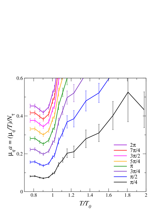
FIG. 6.: Contour plot of the complex phase fluctuation ${\rm STD}(\theta)$ in the $(T/T_{0},\mu_{q}a\equiv(\mu_{q}/T)N_{\tau}^{-1})$ plane. The complex phase $\theta$ contains $O(\mu^{5})$ error. $T_{0}$ is $T_{c}$ at $\mu=0$. $N_{\tau}=4$.

REFERENCES

- [1] F. Karsch and E. Laermann, hep-lat/0305025
- [2] S. Muroya, A. Nakamura, C. Nonaka and T. Takaishi, hep-lat/0306031.
- [3] Z. Fodor and S. Katz, Phys. Lett. B534 (2002) 87; JHEP 0203 (2002) 014.
- [4] C.R. Allton, S. Ejiri, S.J. Hands, O. Kaczmarek, F. Karsch, E. Laermann, Ch. Schmidt and L. Scorzato, Phys. Rev. D66 (2002) 074507.
- [5] Ch. Schmidt, C.R. Allton, S. Ejiri, S.J. Hands, O. Kaczmarek, F. Karsch and E. Laermann, Nucl. Phys. B (Proc. Suppl.) 119 (2003) 517; hep-lat/0309116.
- [6] Z. Fodor, S.D. Katz and K.K. Szabó, Phys. Lett. B568 (2003) 73.
-
[7]
I.M. Barbour and A.J. Bell, Nucl. Phys. B372 (1992) 385;
I.M. Barbour, S.E. Morrison, E.G. Klepfish, J.B. Kogut and M.-P. Lombardo, Phys. Rev. D56 (1997) 7063. - [8] P.R. Crompton, Nucl. Phys. B619 (2001) 499; Nucl. Phys. B626 (2002) 228; hep-lat/0301001.
- [9] A. Roberge and N. Weiss, Nucl. Phys. B275 (1986) 734.
- [10] P. de Forcrand and O. Philipsen, Nucl. Phys. B642 (2002) 290; Nucl. Phys. B673 (2003) 170.
- [11] M. D’Elia and M.-P. Lombardo, Phys. Rev. D67 (2003) 014505.
- [12] S. Choe et al. [QCDTARO collaboration], Phys. Rev. D65 (2002) 054501.
- [13] C.R. Allton, S. Ejiri, S.J. Hands, O. Kaczmarek, F. Karsch, E. Laermann and C. Schmidt, Phys. Rev. D68 (2003) 014507.
- [14] R.V. Gavai and S. Gupta, Phys. Rev. D68 (2003) 034506.
- [15] P. de Forcrand, S. Kim and T. Takaishi, Nucl. Phys. B (Proc. Suppl.) 119 (2003) 541.
- [16] J. Ambjorn, K.N. Anagnostopoulos, J. Nishimura and J.J.M. Verbaarschot, JHEP 0210 (2002) 062.
- [17] A.M. Ferrenberg and R.H. Swendsen, Phys. Rev. Lett. 61 (1988) 2635; Phys. Rev. Lett. 63 (1989) 1195.
- [18] M. Fukugita, M. Okawa and A. Ukawa, Nucl. Phys. B337 (1990) 181.
- [19] Y. Iwasaki et al., Phys. Rev. D46 (1992) 4657.
- [20] S. Ejiri, Y. Iwasaki and K. Kanaya, Phys. Rev. D58, 094505; Nucl. Phys. B (Proc. Suppl.) 73 (1999) 411.
- [21] F. Karsch, Nucl. Phys. B205 (1982) 285.
- [22] G. Burgers, F. Karsch, A. Nakamura and I.O. Stamatescu, Nucl. Phys. B304 (1988) 587.
- [23] J. Engels, F. Karsch and T. Scheideler, Nucl. Phys. B564 (2000) 303.
- [24] T.R. Klassen, Nucl. Phys. B533 (1998) 557.
- [25] U.M. Heller, F. Karsch and B. Sturm, Phys. Rev. D60 (1999) 114502.
- [26] S. Gottlieb, W. Liu, R.L. Renken, R.L. Sugar and D. Toussaint, Phys. Rev. D38 (1988) 2888.
- [27] D.T. Son and M.A. Stephanov, Phys. Rev. Lett. 86 (2001) 592.
- [28] J.B. Kogut and D.K. Sinclair, Phys. Rev. D66 (2002) 034505.
- [29] Y. Hatta and M.A. Stephanov, hep-ph/0302002.
- [30] Y. Sasai, A. Nakamura and T. Takaishi, hep-lat/0310046.
- [31] J.B. Kogut and D.K. Sinclair, Nucl. Phys. B (Proc. Suppl.) 119 (2003) 556; hep-lat/0309042.
- [32] A. Hart, M. Laine and O. Philipsen, Phys. Lett. B505 (2001) 141.
- [33] F. Karsch, E. Laermann and A. Peikert, Phys. Lett. B478 (2000) 447.
- [34] C.R. Allton, hep-lat/9610016; Nucl. Phys. B (Proc. Suppl.) 53 (1997) 867.
- [35] F. Csikor, G.I. Egri, Z. Fodor, S.D. Katz, K.K. Szabó, and A.I. Tóth , hep-lat/0401016.