WUB 03-13
ITP-Budapest 604
Least-Squared Optimized Polynomials for Smeared Link Actions

Abstract

We introduce a numerical method for generating the approximating polynomials used in fermionic calculations with smeared link actions. We investigate the stability of the algorithm and determine the optimal weight function and the optimal type of discretization. The achievable order of polynomial approximation reaches several thousands allowing fermionic calculations using the Hypercubic Smeared Link action even with physical quark masses.

1 Introduction

The usage of smeared or fat links improves flavor symmetry for staggered fermions [1, 2, 3]. Since the smearing contains a projection onto $SU(3)$, the Hypercubic Smeared Link (HYP) action is not bilinear in the original thin link variables. Therefore, the explicit form of the fermion force is rather complicated making the Hybrid Monte-Carlo (HMC) and other molecular dynamics based algorithms with the HYP action practically unusable. An update method based on a stochastic estimator [7, 8] can avoid this problem. The algorithm using improved stochastic estimators [9] requires polynomial approximation of functions of type $x^{-\alpha}e^{p(x)}$, where $\alpha>0$ and $p(x)$ is a low order polynomial. When the calculations are made at the small physical quark masses the order of these polynomials have to be in the range of the thousands. We introduce a numerical method to generate these high order polynomials and investigate the stability, optimal weight function and optimal type of discretization for the algorithm. In contrast to exact methods our procedure is very fast, stable up to thousands of orders and can be applied practically to functions of any type.

The rest of the paper is organized as follows. In the next section we summerize the properties of the HYP action. In Sect. 3 we describe the process of generating the approximating polynomials. We conclude in Sect. 4.

2 The HYP action

The construction of the Hypercubic Smeared Link (HYP) action goes as follows [7, 9]. First, the original thin links $U_{i,\mu}$ are used to construct the set of decorated fat links, $V_{i,\mu;\nu\rho}$ with a modified projected APE blocking step

$$V_{i,\mu;\nu\rho}:=\mathop{\mathrm{missing}}{Proj}\nolimits_{SU(3)}\left[(1-\alpha_{3})U_{i,\mu}+\frac{\alpha_{3}}{2}\sum_{\pm\eta\neq\rho,\nu,\mu}U_{i,\eta}U_{i+\hat{\eta},\mu}U_{i+\hat{\mu},\eta}^{\dagger}\right].$$ (1)

The indices $\nu$ and $\rho$ indicate that the fat link $V_{i,\mu;\nu\rho}$ in direction $\mu$ is not decorated with staples extending in directions $\nu$ and $\rho$. The projection to $SU(3)$ can be defined in two different ways. $W\in SU(3)$ is the deterministic projection of $A$,

$$W=\mathop{\mathrm{missing}}{Proj}\nolimits_{SU(3)}A\quad\text{if}\quad\mathop{\mathrm{missing}}{Re}\mathop{\mathrm{missing}}{Tr}\left(WA^{\dagger}\right)=\max_{U\in SU(3)}\mathop{\mathrm{missing}}{Re}\mathop{\mathrm{missing}}{Tr}\left(UA^{\dagger}\right),$$ (2)

whereas the probabilistic projection $W^{\lambda}$ of $A$ is chosen according to the probability distribution

$$P(W)\propto\exp\left[\frac{\lambda}{3}\mathop{\mathrm{missing}}{Re}\mathop{\mathrm{missing}}{Tr}\left(WA^{\dagger}\right)\right].$$ (3)

In the second step the decorated links $\tilde{V}_{i,\mu;\nu}$ are constructed using the fat links $V_{i,\mu;\nu\rho}$ obtained in the first step as

$$\tilde{V}_{i,\mu;\nu}:=\mathop{\mathrm{missing}}{Proj}\nolimits_{SU(3)}\left[(1-\alpha_{2})U_{i,\mu}+\frac{\alpha_{2}}{4}\sum_{\pm\rho\neq\nu,\mu}V_{i,\rho;\nu\mu}V_{i+\hat{\rho},\mu;\rho\nu}V_{i+\hat{\mu},\rho;\nu\mu}^{\dagger}\right].$$ (4)

In the final step the blocked links $V_{i,\mu}$ are constructed as

$$V_{i,\mu}:=\mathop{\mathrm{missing}}{Proj}\nolimits_{SU(3)}\left[(1-\alpha_{1})U_{i,\mu}+\frac{\alpha_{1}}{6}\sum_{\pm\nu\neq\mu}\tilde{V}_{i,\nu;\mu}\tilde{V}_{i+\hat{\nu},\mu;\nu}\tilde{V}_{i+\hat{\mu},\nu;\mu}^{\dagger}\right].$$ (5)

The smeared link obtained using the above construction containes thin links only from hypercubes attached to the original thin link.

The HYP action is of the form

$$S=S_{g}(U)+\bar{S}_{g}(V)+S_{f}(V),$$ (6)

where $S_{g}(U)$ is the plaquette gauge action

$$S_{g}(U)=-\frac{\beta}{3}\sum_{p}\mathop{\mathrm{missing}}{Re}\mathop{\mathrm{missing}}{Tr}(U_{p})$$ (7)

depending on the thin links $\{U\}$ and $\bar{S}_{g}(V)$ is the gauge action depending on the smeared links $\{V\}$ [9]. The main role of $\bar{S}_{g}(V)$ is to increase the acceptance rate in the accept-reject step. The simplest choice is the smeared plaquette $\bar{S}_{g}(V)=-\frac{\gamma}{3}\sum_{p}\mathop{\mathrm{missing}}{Re}\mathop{\mathrm{missing}}{Tr}(V_{p})$, where $\gamma$ can be tuned to maximize the acceptance rate. The fermions are coupled to the smeared links, thus, the staggered fermionic matrix is of the form

$$M(V)_{i,j}=2m\delta_{i,j}+\sum_{\mu}\eta_{i,\mu}\left(V_{i,\mu}\delta_{i,j-\hat{\mu}}-V_{i-\hat{\mu},\mu}^{\dagger}\delta_{i,j+\hat{\mu}}\right).$$ (8)

The matrix $M(V)^{\dagger}M(V)$ is block diagonal on even and odd lattice sites. Let $\Omega$ denote the even block

$$\Omega(V):=\left(M(V)^{\dagger}M(V)\right)_{\text{even},\text{even}}.$$ (9)

Then the fermionic action $S_{f}(V)$ describing $n_{f}$ flavors is of the form

$$S_{f}(V)=-\frac{n_{f}}{4}\mathop{\mathrm{missing}}{Tr}\ln\Omega(V).$$ (10)

Since the dependence of the smeared links $\{V\}$ on the thin links $\{U\}$ is nonlinear due to the projections to $SU(3)$, the explicit form of the fermionic force, which is needed for molecular dynamics simulations, is very complicated. This fact makes the HMC and R algorithms virtually unusable. A two step algorithm, the partial global stochastic Metropolis update is used instead. In the first step a subset of the thin links $\{U\}$ is updated such that the detailed balance condition with the thin link gauge action $S_{g}(U)$ is satisfied. This can be done using either heatbath or overrelaxation. In the second step the new smeared links $\{V^{\prime}\}$ are computed and the newly obtained configuration is accepted with the probability

$$P_{\text{acc}}=\min\left\{1,\exp\left[-\bar{S}_{g}(V^{\prime})+\bar{S}_{g}(V)\right]\frac{\det\Omega(V^{\prime})}{\det\Omega(V)}\right\}.$$ (11)

Instead of calculating the ratio of the determinants a stochastic estimator is used. The ratio can be expressed as an expectation value

$$\frac{\det\Omega(V^{\prime})}{\det\Omega(V)} = \frac{\displaystyle\int d\xi\xi^{*}\exp\left(-\xi^{*}\Omega(V^{\prime})^{-1}\Omega(V)\xi\right)}{\displaystyle\int d\xi\xi^{*}\exp(-\xi^{*}\xi)}$$ (12)

$$= \left<\exp\left(-\xi^{*}\left[\Omega(V^{\prime})^{-1}\Omega(V)-1\right]\xi\right)\right>_{\xi^{*}\xi}.$$

Only one random source $\xi$ is used on every gauge configuration pair $\{U\}$ and $\{U^{\prime}\}$ to estimate the determinant ratio. The expectation value is taken together with the configuration ensemble average. Then the stochastic acceptance probability becomes

$$P_{\text{stoch}}=\min\left\{1,\exp\left(-\bar{S}_{g}(V^{\prime})+\bar{S}_{g}(V)\right)\exp\left(-\xi^{*}\left[\Omega(V^{\prime})^{-1}\Omega(V)-1\right]\xi\right)\right\}.$$ (13)

If the stochastic estimator has large fluctuations then the acceptance rate can be very small even if the old and new fermionic determinants are almost the same. The standard deviation of the stochastic estimation

$$\left<\exp\left(-\Delta S_{f}\right)\right>=\frac{\det\Omega^{\prime}}{\det\Omega}=\det(A)^{-1}=\left<\exp\left(-\xi^{*}\left[A-1\right]\xi\right)\right>_{\xi^{*}\xi}$$ (14)

can be written in the form

$$\sigma^{2} = \left<\exp\left(-2\xi^{*}\left[A-1\right]\xi\right)\right>_{\xi^{*}\xi}-\left<\exp\left(-\xi^{*}\left[A-1\right]\xi\right)\right>_{\xi^{*}\xi}^{2}$$ (15)

$$= \det\left(2A-1\right)^{-1}-\det(A)^{-2},$$

where $\Omega=\Omega(V)$, $\Omega^{\prime}=\Omega(V^{\prime})$ and $A=\Omega^{\prime-1}\Omega$. As suggested in [10, 11], instead of $\Omega$ and $\Omega^{\prime}$ we introduce the reduced matrices

$$\Omega_{r}=\Omega e^{-2f(\Omega)},\quad\quad\Omega^{\prime}_{r}=\Omega^{\prime}e^{-2f(\Omega^{\prime})},$$ (16)

where $f$ is a polynomial chosen such that the function $e^{2f(x)}/x$ is close to 1 in the interval where the eigenvalues of the matrix $\Omega$ can be found. Then the ratio of the determinants can be rewritten as

$$\frac{\det\Omega^{\prime}}{\det\Omega} = \frac{\det\Omega^{\prime}_{r}}{\det\Omega_{r}}\exp\left(2\mathop{\mathrm{missing}}{Tr}\left[f(\Omega^{\prime})-f(\Omega)\right]\right)$$ (17)

$$= \left<\exp\left(-\xi^{*}\left[\Omega_{r}^{\prime-1}\Omega_{r}-1\right]\xi\right)\right>_{\xi^{*}\xi}\exp\left(2\mathop{\mathrm{missing}}{Tr}\left[f(\Omega^{\prime})-f(\Omega)\right]\right).$$

Since the second factor can be evaluated exactly only the first factor has to be evaluated stochastically. Due to the special choice of $f$, $A_{r}=\Omega_{r}^{\prime-1}\Omega_{r}\approx 1$, so the fluctuations of the stochastic estimator are minimized, improving the acceptance rate.

Equation (15) is valid for the standard deviation of the stochastic estimator only if the matrix $2A-1$ is positive definite, that is, all eigenvalues of $A$ are greater than $1/2$. This is, however, very unlikely if the updating method changes a large number of links of the configuration. In order to avoid this problem the reduced fermionic determinant ratio can be written in the form

$$\det(A_{r})^{-1}=\det\left(A_{r}^{1/n}\right)^{-n}=\left<\exp\left(-\sum_{j=1}^{n}\xi_{j}^{*}\left[A_{r}^{1/n}-1\right]\xi_{j}\right)\right>_{\xi_{j}^{*}\xi_{j}},$$ (18)

where $n$ is an arbitrary positive integer and $\xi_{j}$ are $n$ independent random vectors. Then the standard deviation becomes

$$\sigma^{2}=\det\left(2A_{r}^{1/n}-1\right)^{-n}-\det\left(A_{r}\right)^{-2}.$$ (19)

This is valid only if all the eigenvalues of $A_{r}$ are greater than $2^{-n}$. If $n$ is chosen large enough this condition can always be fulfilled. Since the determinant of a matrix product is independent of the order of the matrices, the $n$th root of $A_{r}$ can be written as

$$A_{r}^{1/n}=\Omega_{r}^{\prime-1/2n}\Omega_{r}^{1/n}\Omega_{r}^{\prime-1/2n}.$$ (20)

The factors can be approximated by polynomials as

$$\Omega_{r}^{\prime-1/2n} = \Omega^{\prime-1/2n}\exp\left(f(\Omega^{\prime})/n\right)=P_{l}^{(2n)}(\Omega^{\prime}),$$

$$\Omega_{r}^{1/n} = \Omega^{1/n}\exp\left(-2f(\Omega)/n\right)=Q_{k}^{(n)}(\Omega).$$ (21)

Here $P_{l}^{(2n)}$ and $Q_{k}^{(n)}$ are $l$ and $k$ order polynomials of the fermionic matrices $\Omega$ and $\Omega^{\prime}$, respectively. Then all the terms of the exponent of (18) can be written in the form

$$\xi^{*}\left[A_{r}^{1/n}-1\right]\xi=\xi^{*}P_{l}^{(2n)}(\Omega^{\prime})Q_{k}^{(n)}(\Omega)P_{l}^{(2n)}(\Omega^{\prime})\xi-\xi^{*}P_{l}^{(2n)}(\Omega^{\prime})Q_{k}^{(n)}(\Omega^{\prime})P_{l}^{(2n)}(\Omega^{\prime})\xi.$$ (22)

The polynomial orders $l$ and $k$ required for a reasonable approximation depend on the used quark mass. The polynomials should be optimized for the interval spanned by the eigenvalues of $\Omega$. The smallest possible eigenvalue is $4m^{2}$, so if smaller and smaller quark masses are used then higher order polynomials are required. The polynomials have to be generated only once before each simulation using the method described in the following section.

3 Generating the polynomials

Our aim is to approximate the function $f$ in the interval $\left[a,b\right]$ using an $n$th order polynomial $P_{f}^{(n)}(x)$. We choose a weight function $w(x)$ and define the deviation of $P_{f}^{(n)}(x)$ from $f$ using the distance in the Hilbert space ${\mathcal{L}_{w^{2}}^{2}\left(\left[a,b\right]\right)}$ as

$$\delta_{n}=\frac{\left\|f-P^{(n)}_{f}\right\|_{w}}{\left\|f\right\|_{w}}=\frac{\displaystyle\sqrt{{\left<f-P_{f}^{(n)},f-P_{f}^{(n)}\right>_{w}}}}{\displaystyle\sqrt{{\left<f,f\right>_{w}}}}=\frac{\displaystyle\sqrt{\displaystyle\mathop{\int}_{a}^{b}\left|f(x)-P_{f}^{(n)}(x)\right|^{2}w(x)^{2}\,\mathrm{d}x}}{\displaystyle\sqrt{\displaystyle\mathop{\int}_{a}^{b}\left|f(x)\right|^{2}w(x)^{2}\,\mathrm{d}x}}.$$ (23)

Here ${\left<,\right>_{w}}$ and $\left\|\,\right\|_{w}$ denote the inner product

$${\left<f,g\right>_{w}}=\displaystyle\mathop{\int}_{a}^{b}f(x)^{*}g(x)w(x)^{2}\,\mathrm{d}x$$ (24)

and the norm

$$\left\|f\right\|_{w}=\sqrt{{\left<f,f\right>_{w}}}$$ (25)

in the Hilbert space ${\mathcal{L}_{w^{2}}^{2}\left(\left[a,b\right]\right)}$, respectively. For the best choice of $w(x)$ see Section 3.2. In order to minimize $\delta_{n}$ we take a basis of orthogonal polynomials $\Phi_{\mu}$,

$${\left<\Phi_{\mu},\Phi_{\nu}\right>_{w}}=\delta_{\mu\nu}q_{\nu},$$ (26)

where $\Phi_{\mu}$ ($\mu=0,1,2,\dots$) is a $\mu$th order polynomial with norm

$$q_{\mu}=\left\|\Phi_{\mu}\right\|_{w}^{2}=\displaystyle\mathop{\int}_{a}^{b}\left|\Phi_{\mu}(x)\right|^{2}w(x)^{2}\,\mathrm{d}x.$$ (27)

This basis of polynomials is generated using the Gram-Schmidt orthogonalization process from the simple polynomials $\mathop{\mathrm{id}}\nolimits^{0}\,(\equiv\!1)$, $\mathop{\mathrm{id}}\nolimits^{1}\,(\equiv\!x)$, $\mathop{\mathrm{id}}\nolimits^{2}\,(\equiv\!x^{2})$, …:

$$\Phi_{0} := \mathop{\mathrm{id}}\nolimits^{0}=1$$

$$\Phi_{1} := \left(I-\frac{{\left|\Phi_{0}\right>\!\left<\Phi_{0}\right|_{w}}}{\left\|\Phi_{0}\right\|_{w}^{2}}\right)\mathop{\mathrm{id}}\nolimits^{1}=\mathop{\mathrm{id}}\nolimits^{1}-\frac{{\left<\Phi_{0},\mathop{\mathrm{id}}\nolimits^{1}\right>_{w}}}{q_{0}}\,\Phi_{0}$$

$$\Phi_{2} := \left(I-\frac{{\left|\Phi_{0}\right>\!\left<\Phi_{0}\right|_{w}}}{\left\|\Phi_{0}\right\|_{w}^{2}}-\frac{{\left|\Phi_{1}\right>\!\left<\Phi_{1}\right|_{w}}}{\left\|\Phi_{1}\right\|_{w}^{2}}\right)\mathop{\mathrm{id}}\nolimits^{2}=\mathop{\mathrm{id}}\nolimits^{2}-\frac{{\left<\Phi_{0},\mathop{\mathrm{id}}\nolimits^{2}\right>_{w}}}{q_{0}}\,\Phi_{0}-\frac{{\left<\Phi_{1},\mathop{\mathrm{id}}\nolimits^{2}\right>_{w}}}{q_{1}}\,\Phi_{1}$$

$$\Phi_{\mu+1} := \left(I-\sum_{\nu=0}^{\mu}\frac{{\left|\Phi_{\nu}\right>\!\left<\Phi_{\nu}\right|_{w}}}{\left\|\Phi_{\nu}\right\|_{w}^{2}}\right)\mathop{\mathrm{id}}\nolimits^{\mu+1}=\mathop{\mathrm{id}}\nolimits^{\mu+1}-\sum_{\nu=0}^{\mu}\frac{1}{q_{\nu}}{\left<\Phi_{\nu},\mathop{\mathrm{id}}\nolimits^{\mu+1}\right>_{w}}\Phi_{\nu}.$$ (28)

Using this basis $f$ can be written as

$$f=\sum_{\mu=0}^{\infty}\frac{{\left<\Phi_{\mu},f\right>_{w}}}{{\left<\Phi_{\mu},\Phi_{\mu}\right>_{w}}}=\sum_{\mu=0}^{\infty}\frac{b_{\mu}}{q_{\mu}}\Phi_{\mu},$$ (29)

where

$$b_{\mu}:={\left<\Phi_{\mu},f\right>_{w}}=\displaystyle\mathop{\int}_{a}^{b}\Phi_{\mu}(x)f(x)w(x)^{2}\,\mathrm{d}x.$$ (30)

The $n$th order polynomial $P_{f}^{(n)}$ for which $\delta_{n}$ is minimal can be obtained by taking only the first $n$ terms of the sum in (29).

$$P_{f}^{(n)}:=\sum_{\mu=0}^{n}\frac{b_{\mu}}{q_{\mu}}\Phi_{\mu}=\sum_{\mu=0}^{n}c_{\mu}\Phi_{\mu},\quad\quad c_{\mu}:=\frac{b_{\mu}}{q_{\mu}}$$ (31)

In order to obtain the polynomials $\Phi_{\mu}$ a second order recursion formula [12, 13] can be used instead of the numerically unstable Gram-Schmidt orthogonalization process (28). The recursion goes as follows. The first two polynomials are obtained identically according to (28)

$$\Phi_{0}(x)=1,\quad\quad\Phi_{1}(x)=x-\frac{\displaystyle\displaystyle\mathop{\int}_{a}^{b}w(x)^{2}x\,\mathrm{d}x}{\displaystyle\displaystyle\mathop{\int}_{a}^{b}w(x)^{2}\,\mathrm{d}x}.$$ (32)

Let

$$p_{\mu}:=\displaystyle\mathop{\int}_{a}^{b}\Phi_{\mu}(x)^{2}w(x)^{2}x\,\mathrm{d}x$$ (33)

and

$$\beta_{\mu}:=-\frac{p_{\mu}}{q_{\mu}},\quad\gamma_{\mu-1}:=-\frac{q_{\mu}}{q_{\mu-1}}.$$ (34)

Then the rest of the polynomials can be obtained as

$$\Phi_{\mu+1}(x)=(x+\beta_{\mu})\Phi_{\mu}(x)+\gamma_{\mu-1}\Phi_{\mu-1}(x).$$ (35)

3.1 Numerical realization

One proper method of proceeding with the algorithm is to calculate the integrals (27), (30) and (33) exactly. This method is followed in Ref. [14]. These calculations require a precision of several hundreds or thousands of digits which can be carried out using multiprecision arithmetics libraries. Since the integrals are carried out exactly the indefinite integrals of the integrands have to be known. As a consequence only special types of functions $f$ can be approximated and the weight function $w$ also has to be carefully chosen.

The method we use is to calculate the integrals numerically. The interval $\left[a,b\right]$ is divided into N subintervals (N+1 discretization points) logarithmically (see Section 3.2). Since all the integrals are calculated using Simpson’s rule, N has to be even. The values of the function $f$, polynomials $\Phi_{\mu}$ and the weight function $w^{2}$ are calculated and stored only at the discretization points. First $\Phi_{0}$ and $\Phi_{1}$ are determined with the integrals in (32) carried out numerically. In the $\mu$th step $q_{\mu}$ and $p_{\mu}$ are calculated first using (27) and (33), then $\beta_{\mu}$ and $\gamma_{\mu-1}$ using (34). Then $\Phi_{\mu+1}$ is determined at each discretization point from $\Phi_{\mu}$ and $\Phi_{\mu-1}$ using (35). Then $b_{\mu}$ and $c_{\mu}$ are calculated using (30). Finally, $c_{\mu}\cdot\Phi_{\mu}$ is added to the actual value of $P_{f}^{(n)}$.

This method has three major advantages. Firstly, we have a second order recursion formula (35). Therefore, at each step only the last two orthogonal polynomials have to be stored in memory. That is, the memory required for the calculations depends only on the number of discretization points $N$ but is independent of the order of approximation. Secondly, no multiprecision arithmetics is needed. All the calculations can be carried out using the built in 10 Byte floating point type. Finally, since the integrals are evaluated numerically, the indefinite integrals of the integrands are not needed. Therefore, there are no restrictions on the form of the function $f$ and the weight function $w$.

3.2 Stability, optimal weight function and discretization

In order to describe the numerical stability of the recursion formula (35) and to find the optimal weight function $w$ and the optimal type of discretization we need to refer to ${\mathcal{L}^{2}\left(\left[a,b\right]\right)}$, the Hilbert space of $\left[a,b\right]\to\mathbb{C}\,$ square-integrable functions with the inner product ${\left<f,g\right>}=\int_{a}^{b}f(x)^{*}g(x)\,\mathrm{d}x$. If the weight function $w$ is such that

$$0<\kappa_{1}<w(x)<\kappa_{2}\quad\forall x\in\left[a,b\right],$$ (36)

then the equivalence classes in ${\mathcal{L}^{2}\left(\left[a,b\right]\right)}$ consist of the same functions as in ${\mathcal{L}_{w^{2}}^{2}\left(\left[a,b\right]\right)}$ and ${\mathcal{L}^{2}\left(\left[a,b\right]\right)}$ consist of the same equivalence classes as ${\mathcal{L}_{w^{2}}^{2}\left(\left[a,b\right]\right)}$. That is, ${\mathcal{L}_{w^{2}}^{2}\left(\left[a,b\right]\right)}$ and ${\mathcal{L}^{2}\left(\left[a,b\right]\right)}$ are identical as linear spaces.

Both

$$\Big{\{}e_{n}\Bigm{|}n\in\mathbb{Z}\Big{\}}$$ (37)

and

$$\Big{\{}s_{n}\Bigm{|}n\in\mathbb{N}\Big{\}}\cup\Big{\{}c_{n}\Bigm{|}n\in\mathbb{N}\Big{\}}\cup\Big{\{}c_{0}\Big{\}}$$ (38)

form orthonormal bases in ${\mathcal{L}^{2}\left(\left[a,b\right]\right)}$, where

$$e_{n}(x)=\frac{1}{\sqrt{b-a}}\exp\left[\frac{2\pi ni}{b-a}\left(x-\frac{a+b}{2}\right)\right],\quad\quad n=\dots,-2,-1,0,1,2,\dots$$ (39)

and

$$s_{n}(x) = \sqrt{\frac{2}{b-a}}\sin\left[\frac{2\pi n}{b-a}\left(x-\frac{a+b}{2}\right)\right],\quad\quad n=1,2,3,\dots$$

$$c_{n}(x) = \sqrt{\frac{2}{b-a}}\cos\left[\frac{2\pi n}{b-a}\left(x-\frac{a+b}{2}\right)\right],\quad\quad n=1,2,3,\dots$$ (40)

$$c_{0}(x) = \frac{1}{\sqrt{b-a}}=e_{0}(x).$$

Using these basis vectors the linear map

$$F:=I+i\cdot\mathop{\mathrm{missing}}{(s)\!\!}\sum\limits_{n=1}^{\infty}\Big{(}{\left|s_{n}\right>\!\left<c_{n}\right|}-{\left|c_{n}\right>\!\left<s_{n}\right|}\Big{)}={\left|e_{0}\right>\!\left<e_{0}\right|}+2\cdot\mathop{\mathrm{missing}}{(s)\!\!}\sum\limits_{n=1}^{\infty}{\left|e_{n}\right>\!\left<e_{n}\right|}$$ (41)

can be defined, which is bounded and self-adjoint in ${\mathcal{L}^{2}\left(\left[a,b\right]\right)}$. Let

$$A_{f}(x):=\big{|}\big{(}Ff\big{)}(x)\big{|}$$ (42)

and

$$\varphi_{f}(x):=\arg\bigg{(}\big{(}Ff\big{)}(x)\bigg{)}.$$ (43)

Then

$$\big{(}Ff\big{)}(x)=A_{f}(x)\cdot\exp\left(i\varphi_{f}(x)\right).$$ (44)

If $f$ is real, then

$$f(x)=\mathop{\mathrm{missing}}{Re}\bigg{(}\big{(}Ff\big{)}(x)\bigg{)}=A_{f}(x)\cdot\cos\left(\varphi_{f}(x)\right).$$ (45)

That is, $A_{f}(x)$ and $\varphi_{f}(x)$ can be naturally identified as the amplitude and phase of the real function $f$ at point $x$, respectively. If $\varphi_{f}$ is differentiable then we can define

$$\varrho_{f}(x):=\frac{1}{\pi}\varphi_{f}^{\prime}(x).$$ (46)

If $f$ is a polynomial without multiple zeros (which is the case when dealing with orthogonal polynomials) then $\varphi_{f}$ is strictly increasing and $\varrho_{f}>0$. In this case if

$$\mathop{\int}_{x_{1}}^{x_{2}}\varrho_{f}(x)\,\mathrm{d}x=k$$ (47)

for some $a<x_{1}<x_{2}<b$, then $f$ has exactly $k$ zeros in both $\left[x_{1},x_{2}\right[$ and $\left]x_{1},x_{2}\right]$. Thus, $\varrho_{f}$ can be identified as the density or root density of polynomial $f$. Graphically speaking, $A_{f}(x)$ describes the ’amplitude’ of the polynomial $f$ at point $x$ and $\varrho_{f}(x)$ describes the ’rate at which the polynomial $f$ oscillates’ near $x$ (Figure 1). If $f_{1}$ and $f_{2}$ are polynomials without multiple zeros such that $f_{1}$ and $f_{2}$ have no common zeros, then the number of roots of $f_{1}\cdot f_{2}$ in every $\left[x_{1},x_{2}\right]\subset\left[a,b\right]$ is equal to the sum of the number of roots of $f_{1}$ and $f_{2}$ in that interval. Therefore, the root density of such a product is approximately the sum of the root density of the factors.

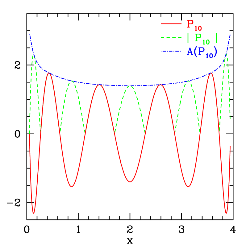
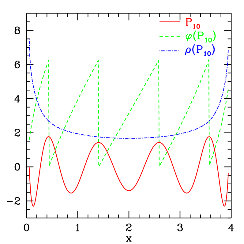
Figure 1: The amplitude (left), phase and density (right) of the 10th orthogonal polynomial $P_{10}$ with respect to the weight function $w=1$ on the interval $\left[0,4\right]$.

Let $\Phi_{\mu}$ and $P_{\mu}$ denote the $\mu$th orthogonal polynomials in ${\mathcal{L}_{w^{2}}^{2}\left(\left[a,b\right]\right)}$ and ${\mathcal{L}^{2}\left(\left[a,b\right]\right)}$, respectively. If $a=-1$ and $b=1$ then the polynomials $P_{\mu}$ are equal to the Legendre polynomials. Using the formulae for the asymptotic behaviour of the Legendre polynomials [15, §8.21] the formula

$$A_{P_{\mu}}(x)=\text{const}\cdot\frac{1}{\displaystyle\sqrt[4]{\left(\frac{b-a}{2}\right)^{2}-\left(x-\frac{a+b}{2}\right)^{2}}}+O(\mu^{-3/2})$$ (48)

can be obtained for the amplitude $A_{P_{\mu}}$ of the polynomials $P_{\mu}$ for large $\mu$s.

If $w$ satisfies condition (36), then

$$w(x)A_{\Phi_{\mu}}(x)\approx\text{const}\cdot A_{P_{\mu}}(x)$$ (49)

for large $\mu$s, that is, for large $\mu$s the amplitude of $\Phi_{\mu}$ can be well approximated by

$$A_{\Phi_{\mu}}(x)\approx\text{const}\cdot\frac{1}{w(x)}A_{P_{\mu}}(x),$$ (50)

where the constant is independent of $x$ and is near $1$ (Figure 2). Combining equations (48) and (50) the amplitude of the $\mu$th orthogonal polynomial $\Phi_{\mu}$ can be approximately given by the formula

$$A_{\Phi_{\mu}}(x)\approx\text{const}\cdot\frac{1}{w(x)}\,\frac{1}{\displaystyle\sqrt[4]{\left(\frac{b-a}{2}\right)^{2}-\left(x-\frac{a+b}{2}\right)^{2}}}=:A_{w}(x).$$ (51)

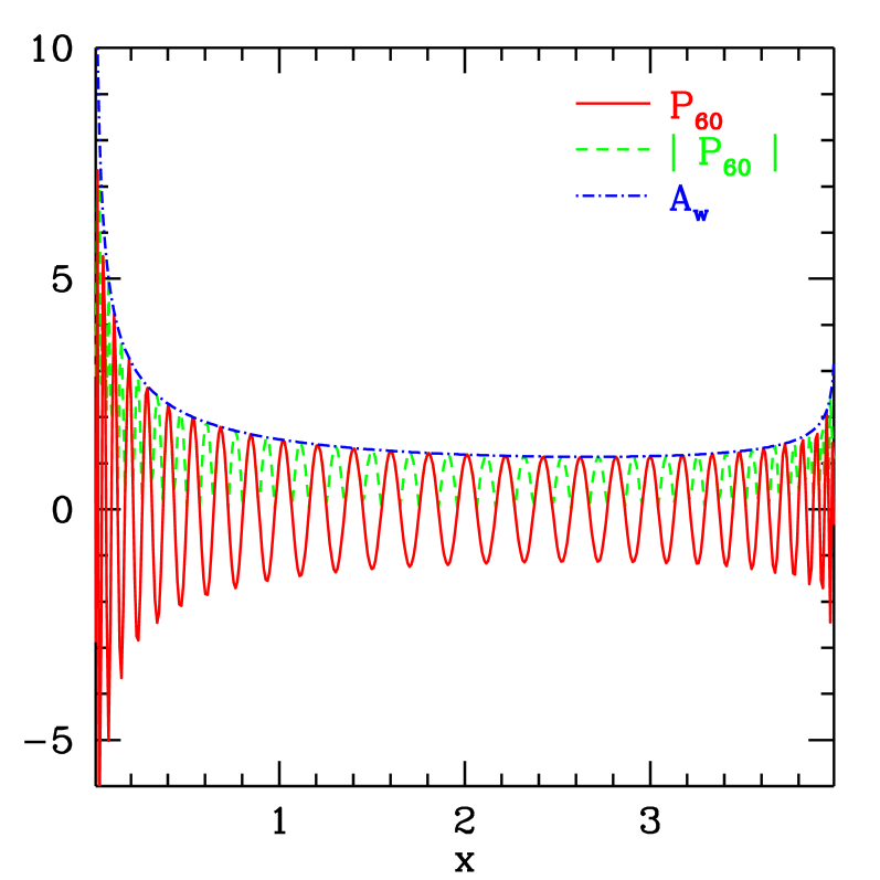
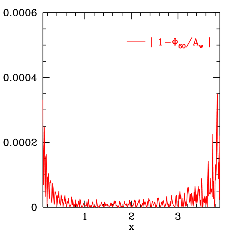
Figure 2: Left: $A_{w}$, defined in equation (51), as the amplitude of $\Phi_{60}$. Right: The relative deviation of the amplitude of $\Phi_{60}$ and $A_{w}$ with $a=10^{-5}$, $b=4$ and $w(x)=x^{-1/4}$. (The amplitude of $\Phi_{60}$ was calculated numerically using only the first 5000 terms of the sum in equation (41).)

For large $\mu$s the root density of the polynomials can be approximated by

$$\varrho_{\Phi_{\mu}}(x)\approx\mu\,\omega_{\mu}\cdot\frac{\displaystyle\frac{1}{\pi}}{\displaystyle\sqrt{\left(\frac{b-a}{2}\right)^{2}-\left(x-\frac{a+b}{2}\right)^{2}}}=:\mu\,\omega_{\mu}\cdot\varrho(x),$$ (52)

where $\omega_{\mu}$ depends on the weight function $w$. In all cases $\omega_{\mu}$ is close to 1 and $\displaystyle\lim_{\mu\to\infty}\omega_{\mu}=1$ (Figure 3).

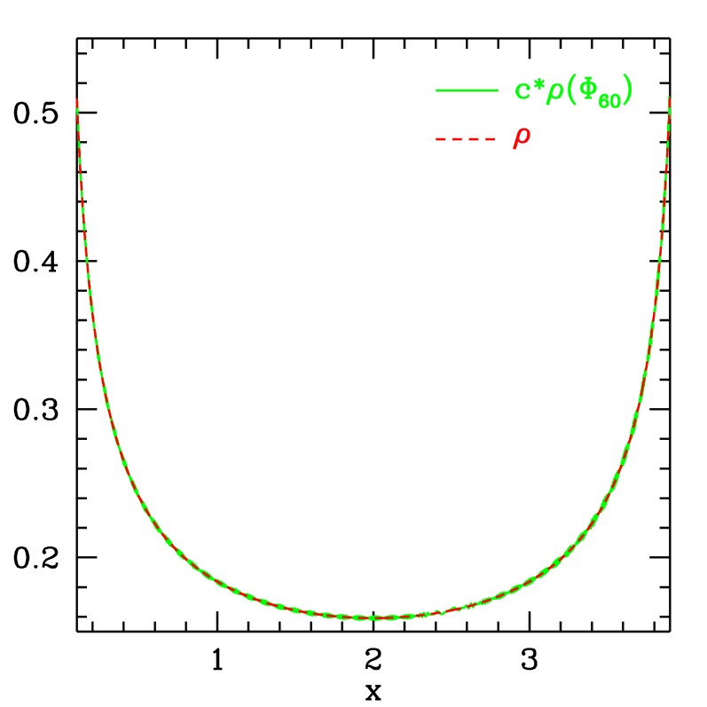
Figure 3: $\frac{1}{60}\cdot 0.9875\cdot\varrho_{\Phi_{60}}(x)$ calculated numerically (solid line) such that only the first 5000 terms of the sum in equation (41) were taken into account and $\varrho(x)$ (dashed line) with $a=10^{-5}$, $b=4$ and $w(x)=x^{-1/4}$.

With

$$\varphi(x):=\pi\displaystyle\mathop{\int}_{a}^{x}\varrho(z)\,\mathrm{d}z=\pi-\arccos\left(\frac{2x-a-b}{b-a}\right)$$ (53)

and using equations (45), (51) and (52) we can conclude at

$$\Phi_{\mu}(x)\approx A_{w}(x)\cdot\cos\left\{\mu\,\omega_{\mu}\left[\pi-\arccos\left(\frac{2x-a-b}{b-a}\right)\right]\right\}=:F_{w,\mu}(x),$$ (54)

an approximate formula for the $\mu$th orthogonal polynomial with respect to the weight fuction $w$ (Figure 4).

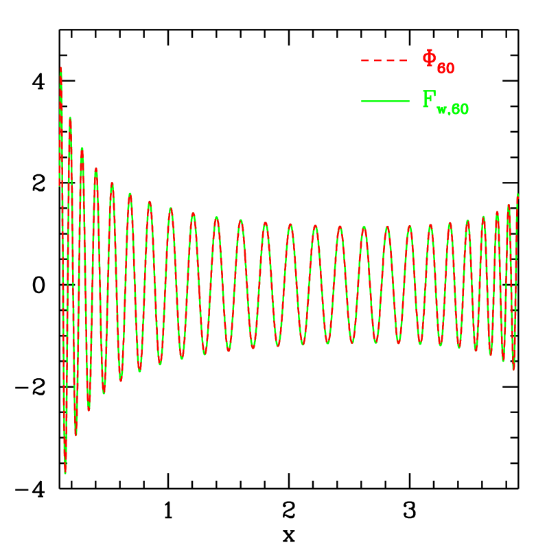
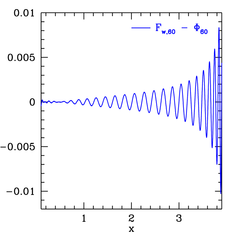
Figure 4: Left: $F_{w,60}$ (solid line) with $\omega_{60}=0.9875$ and $\Phi_{60}$ (dashed line). Right: The difference of $F_{w,60}$ and $\Phi_{60}$. ($a=10^{-5}$, $b=4$ and $w(x)=x^{-1/4}$)

We use Simpson’s rule in order to calculate the integrals (27), (30) and (33) numerically. The numerical integral of the function $g$ taken over the discretization interval $I=\left[z-h,z+h\right]$ is

$$\int_{I,\text{num.}}g=\left[\frac{1}{3}g(z-h)+\frac{4}{3}g(z)+\frac{1}{3}g(z+h)\right]h.$$ (55)

Assume that $g$ is analytic in $I$ with radius of convergence at $z$ greater then $h$, that is,

$$g(z+u)=\sum_{n=0}^{\infty}\frac{g^{(n)}(z)}{n!}\,u^{n}\quad\quad-h\leq u\leq h.$$ (56)

The exact integral and the numerical integral of $g$ then becomes

$$\int_{I}g=\sum_{n=0}^{\infty}\frac{g^{(n)}(z)}{n!}\,\frac{h^{n+1}}{n+1}-\sum_{n=0}^{\infty}\frac{g^{(n)}(z)}{n!}\,\frac{(-h)^{n+1}}{n+1}=2\sum_{k=0}^{\infty}\frac{g^{(2k)}(z)}{(2k+1)!}\,h^{2k+1}$$ (57)

and

$$\int_{I,\text{num.}}g = \left[\frac{1}{3}\sum_{n=0}^{\infty}\frac{g^{(n)}(z)}{n!}\,(-h)^{n}+\frac{4}{3}\sum_{n=0}^{\infty}\frac{g^{(n)}(z)}{n!}\,(0)^{n}+\frac{1}{3}\sum_{n=0}^{\infty}\frac{g^{(n)}(z)}{n!}\,h^{n}\right]h=$$ (58)

$$= \left[\frac{2}{3}\sum_{k=0}^{\infty}\frac{g^{(2k)}(z)}{(2k)!}\,h^{2k}+\frac{4}{3}g(z)\right]h,$$

respectively. Then the error of integration over the interval $I$, that is, the difference of the exact and the numerical integrals becomes

$$\Delta_{I}g=\left|\int_{I}g-\int_{I,\text{num.}}g\right|=\left|\sum_{k=2}^{\infty}\frac{g^{(2k)}(z)}{(2k)!}\,\left(\frac{2}{3}-\frac{2}{2k+1}\right)h^{2k+1}\right|.$$ (59)

If $h$ is small enough and $\mu$ is large enough such that $\Phi_{\mu}$ oscillates much faster than $w$ and $f$ the integrand of (30) can be approximated on $I$ by

$$F_{z}(u):=B(z)\cos\left(\pi\,\mu\,\varrho(z)\cdot u+\varphi_{\Phi_{\mu}}(z)\right)\quad\quad-h\leq u\leq h,$$ (60)

where $B(z)=w(z)^{2}f(z)A_{\Phi_{\mu}}(z)$.

$$F_{z}^{(2k)}(u)=(-1)^{k}\left(\pi\,\mu\,\varrho(z)\right)^{2k}\cdot F_{z}(u),$$ (61)

thus, the error of integrating $F_{z}$ numerically over $I$ can be estimated as

$$\Delta_{I}F_{z} = \left|F_{z}(z)\right|\cdot\left|\sum_{k=2}^{\infty}\frac{(-1)^{k}\left(\pi\,\mu\,\varrho(z)\right)^{2k}}{(2k)!}\,\left(\frac{2}{3}-\frac{2}{2k+1}\right)h^{2k+1}\right|\leq\frac{2}{3}h\left|F_{z}(z)\right|\sum_{k=2}^{\infty}\frac{\left(\pi\,\mu\,\varrho(z)\right)^{2k}h^{2k}}{(2k)!}$$ (62)

$$\leq \frac{2}{3}h\left|B(z)\right|\cdot\left[\cosh\left(\pi\,\mu\,\varrho(z)\,h\right)-1-\frac{\left(\pi\,\mu\,\varrho(z)\,h\right)^{2}}{2}\right]$$

$$\approx \frac{1}{36}h\left|B(z)\right|\left(\pi\,\mu\,\varrho(z)\,h\right)^{4}\cdot\left[1+O\left(\left(\pi\,\mu\,\varrho(z)\,h\right)^{2}\right)\right].$$

$1/\left(\pi\,\mu\,\varrho(z)\,h\right)$ shows the number of discretization points between two consecutive zeros of $\Phi_{\mu}$ near $z$. The density of discretization has to be chosen such that the relative error

$$\delta_{I}F_{z}=\frac{\displaystyle\Delta_{I}F_{z}}{\displaystyle\left|B(z)\right|\cdot h}$$ (63)

of the numerical integration is in the same order of magnitude in each discretization interval and is equal to the desired relative error of the numerical integration over $\left[a,b\right]$.

Since $\cos^{2}x=(1+\cos 2x)/2$ and the integrands in (27) and (33) contain the square of $\Phi_{\mu}$, they can be treated as a constant plus a cosine of double frequency in every discretization interval. The error of the numerical integration can be estimated similarly, leading us to the same conclusion.

If $f$ is not continuous on $\left[a,b\right]$, then the convergence in (29) is not uniform but an almost everywhere convergence. Assume that $f$ has an $(x-a)^{-\alpha}$ type ($\alpha>0$) singularity near $a$, that is, $\displaystyle 0<\left|\lim_{x\to a^{+}}f(x)(x-a)^{\alpha}\right|<\infty$. Then the closer we get to $a$ the slower the convergence becomes. Thus, by taking into account only a finite number of terms in (29) we can get a reasonable approximation for $f$ only in $\left[a+\epsilon,b\right]$ with a suitably chosen $\epsilon$. The procedure in this case should be as follows. We need to determine the size $\epsilon$ of the neighborhood of $a$ in which the approximation of $f$ is not needed. Then we generate the orthogonal polynomials using (35) in the interval $\left[a^{\prime}=a+\epsilon,b\right]$ and calculate the approximating polynomial $P_{f}^{(n)}$ with the desired degree of approximation $n$.

If $f$ does not have singularities and is continuous on $\left[a,b\right]$ then the weight function $w$ can be chosen to be an arbitrary continuous function. If $f$ has singularities, for example an $(x-a)^{-\alpha}$ type singularity near $a$, then the best choice for $w$ is as follows. $w$ should have an $(x-a)^{\alpha}$ type behaviour near $a$ and should be a smooth function otherwise. If $f$ is such that $\left|f(x)\right|>\kappa>0\,\,\,\forall x\in\left]a,b\right]$ then the best choice is $w(x)=1/\left|f(x)\right|$. Choosing $w$ in such a way has the following advantages. 1. According to (50) the amplitude of the polynomials $\Phi_{\mu}$ will gain approximately the same type of singularity as $f$ has, therefore, the relative deviation of $f$ and $P_{f}^{(n)}$ is decreasing uniformly. 2. In the integrand of equation (30) the singularity of $f$ is cancelled out by one of the two $w$’s, while the other $w$ deals with $\Phi_{\mu}$ according to (50).

In order to find the optimal type of discretization of interval $\left[a,b\right]$ we need to consider both the singularities and the densities of the integrands (27), (33) and (30). Taking (48) and (50) into account we can conclude that $\left|B(x)\right|$ of (27) and (33) (see (62)) has singularities near $a$ and $b$ of type $1/\sqrt{x-a}$ and $1/\sqrt{b-x}$, respectively, and (30) has singularities of type $1/\sqrt[4]{x-a}$ and $1/\sqrt[4]{b-x}$. The densities of all three integrands are of type $1/\sqrt{(x-a)(b-x)}$. As a consequence, the optimal discretization should contain the discretization points with density proportional to $1/[(x-a)(b-x)]$. This would require infinitely many discretization points, thus, we choose a small $\epsilon$ and discretize the interval $I^{\prime}=\left[a^{\prime},b^{\prime}\right]=\left[a+\epsilon,b-\epsilon\right]$ with the above density. If we use $N$ discretization points, then the discretization interval $\left[z-h_{z},z+h_{z}\right]$ at $z$ has the length

$$2h_{z}=\left\{\begin{matrix}\displaystyle(z-a)\left[\left(\frac{b-a}{2\epsilon}\right)^{4/N}-1\right]\quad\quad\text{if}\quad a+\epsilon\leq z\leq\frac{a+b}{2}\\ \displaystyle(b-z)\left[\left(\frac{b-a}{2\epsilon}\right)^{4/N}-1\right]\quad\quad\text{if}\quad\frac{a+b}{2}\leq z\leq b-\epsilon.\\ \end{matrix}\right.$$ (64)

The length of the longest and shortest intervals of this logarithmic discretization is $\frac{\epsilon}{2}\left[\left(\frac{b-a}{2\epsilon}\right)^{4/N}-1\right]$ and $\frac{b-a}{4}\left[\left(\frac{b-a}{2\epsilon}\right)^{4/N}-1\right]$, respectively.

In the usual fermionic calculations $a=0$ and the functions of the fermionic matrix that have to be evaluated have singularities of type $x^{-\alpha}$ ($\alpha>0$) at $x=0$. We use the above polynomial expansion to approximate these singular functions. $\epsilon$ should be chosen such that all eigenvalues of the fermionic matrix are greater then $\epsilon$. The smallest eigenvalue of the fermionic matrix is proportional to the square of the quark mass. Since our aim is to use quark masses as low as the physical $u,d$ quark masses, which are approximately $m_{ud}=0.002$ in lattice mass units, $\epsilon$ should be in the order of magnitude of $10^{-6}$. In order to be able to well approximate the functions of the fermionic matrix so close to their singularities the required order of polynomial approximation is in the thousands.

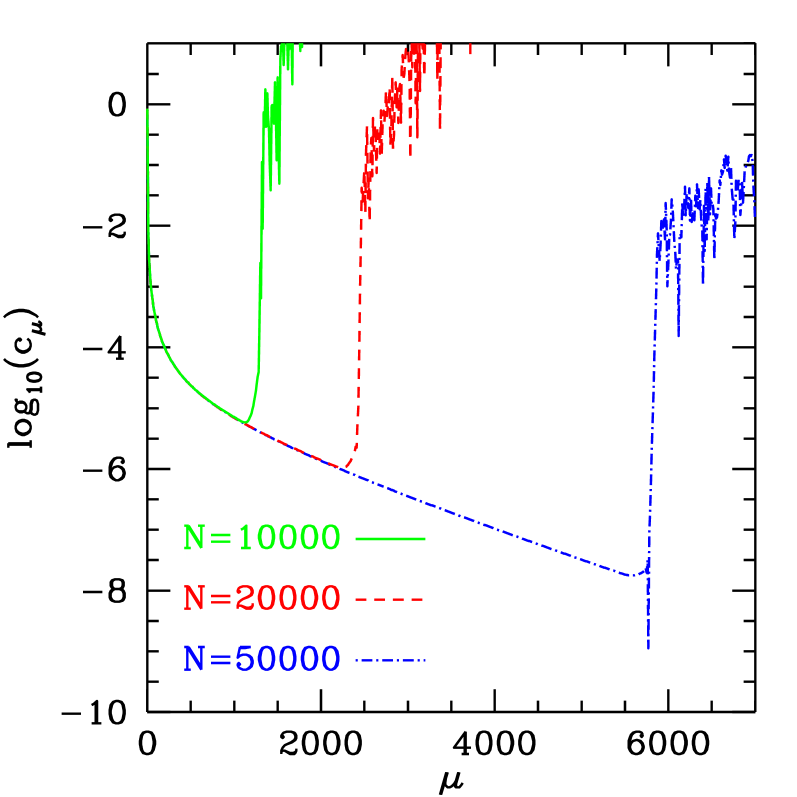
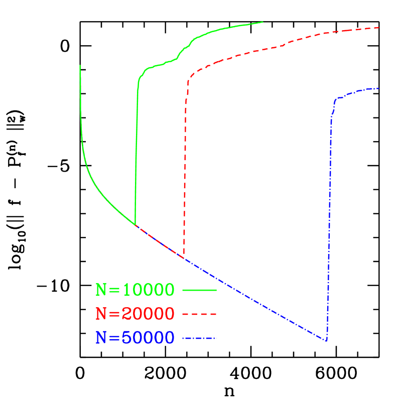
Figure 5: The logarithm of the coefficients $c_{\mu}$ (left) and the deviations $\left\|f-P_{f}^{(n)}\right\|_{w}^{2}$ (right) as the function of the order with number of discretization points $N=10000$, $N=20000$ and $N=50000$.

Using this logarithmic type of discretization the order $n$ up to which the algorithm (35) is stable can be tested. The coefficients $c_{\mu}$ and the deviations $\left\|f-P_{f}^{(n)}\right\|_{w}^{2}$ can be seen in Figure 5, when the approximated function is chosen to be $f=x^{-1/4}$, $a=0$, $b=4$ and $\epsilon=10^{-6}$. It can be verified that the algorithm is stable approximately up to the orders $n=1000$, $n=2000$ and $n=5500$ if the numbers of discretization points are $N=10000$, $N=20000$ and $N=50000$, respectively. Since no multiprecision arithmetics is required for the algorithm, its CPU time and memory requirements are considerably low. Generating the polynomials up to the order of $n=5500$ in the case of $N=50000$ takes approx. 2.5 minutes of CPU time on a $1.6\,\text{GHz}$ AMD Athlon processor and requires approx. $5\,\text{MB}$ of RAM.

4 Conclusion

We have introduced an alternate numerical method for generating the approximating polynomials used in fermionic calculations with smeared link actions. This algorithm was based on the idea of calculating all the integrals numerically and calculating and storing all the functions and polynomials only at finitely many discretization points. The advantages of this algorithm include memory usage independent of the order of approximation, unnecessarity of multiprecision arithmetics libraries and the absence of restrictions for the form of the approximated and the weight functions. We investigated the stability of the algorithm and based on the asymptotic behaviour of the orthogonal polynomial base appearing in the method we determined the optimal weight function and the optimal type of discretization. As a result the achievable order of polynomial approximation reached several thousands which is essential for fermionic calculations near the small physical quark masses.

5 Acknowledgments

We thank Ferenc Csikor, Zoltán Fodor and István Montvay for useful discussions and careful reading of the manuscript. This work was partially supported by Hungarian Scientific grants, OTKA-T37615/T34980.

References

- [1] G. P. Lepage, Phys. Rev. D 59, 074502 (1999) [arXiv:hep-lat/9809157].
- [2] K. Orginos, D. Toussaint and R. L. Sugar [MILC Collaboration], Phys. Rev. D 60, 054503 (1999) [arXiv:hep-lat/9903032].
- [3] A. Hasenfratz and F. Knechtli, Phys. Rev. D 64, 034504 (2001) [arXiv:hep-lat/0103029].
- [4] W. Kamleh, D. B. Leinweber and A. G. Williams, arXiv:hep-lat/0309154.
- [5] J. M. Zanotti et al. [CSSM Lattice Collaboration], Phys. Rev. D 65 (2002) 074507 [arXiv:hep-lat/0110216].
- [6] C. Morningstar and M. J. Peardon, arXiv:hep-lat/0311018.
- [7] F. Knechtli and A. Hasenfratz, Phys. Rev. D 63, 114502 (2001) [arXiv:hep-lat/0012022].
- [8] A. Hasenfratz and F. Knechtli, Comput. Phys. Commun. 148, 81 (2002) [arXiv:hep-lat/0203010].
- [9] A. Hasenfratz and A. Alexandru, Phys. Rev. D 65, 114506 (2002) [arXiv:hep-lat/0203026].
- [10] M. Hasenbusch, Phys. Rev. D 59, 054505 (1999) [arXiv:hep-lat/9807031].
- [11] P. de Forcrand, Nucl. Phys. Proc. Suppl. 73 (1999) 822 [arXiv:hep-lat/9809145].
- [12] I. Montvay, arXiv:hep-lat/9903029.
- [13] I. Montvay, arXiv:hep-lat/9911014.
- [14] C. Gebert and I. Montvay, arXiv:hep-lat/0302025.
- [15] Gabor Szegő: Orthogonal Polynomials, American Mathematical Society Colloquium Publications, Vol 23, 4th Ed, Providence, RI, 1975