Computing the $\eta$ and $\eta^{\prime}$ Mesons in Lattice QCD

Abstract

It has been known for a long time that the large experimental singlet-octet mass gap in the pseudoscalar meson mass spectrum originates from the anomaly of the axial vector current, i.e. from nonperturbative effects and the nontrivial topological structure of the QCD vacuum. In the $N_{colour}\rightarrow\infty$ limit of the theory, this connection elucidates in the famous Witten-Veneziano relation between the $\eta^{\prime}$-mass and the topological susceptibility of the quenched QCD vacuum. While lattice quantum chromodynamics (LQCD) has by now produced impressive high precision results on the flavour nonsinglet hadron spectrum, the determination of the pseudoscalar singlet mesons from direct correlator studies is markedly lagging behind, due to the computational complexity in handling observables that include OZI-rule violating diagrams, like the $\eta^{\prime}$ propagator. In this article we report on some recent progress in dealing with this numerical bottleneck problem.

1 Introduction

Long before the advent of QCD as the field theory of strong interactions, the $\pi$-meson has been allocated the rôle of the Goldstone Boson in a near-chiral world of light quarks while its flavour singlet partner, the $\eta^{\prime}$ meson, was thought to acquire its nearly baryonic mass of $960$ MeV through ultraviolet quantum fluctuations that prevent the flavour singlet axial vector current

$$j_{5}^{\mu(0)}(x)=\bar{q}(x)\gamma_{5}\gamma^{\mu}q(x)$$ (1)

from being conserved, even in the massless theory. In this scenario the breaking of $SU(3)_{L}\times SU(3)_{R}$ chiral symmetry occurs as a renormalization effect within a Wilson expansion of the operator $\partial_{\mu}j_{5}^{\mu(0)}$ that suffers operator mixing with the topological charge density

$$Q(x)=(g^{2}/32\pi^{2})\;\mbox{tr}F(x)^{\alpha\beta}F^{D}_{\alpha\beta}(x)$$ (2)

in the form

$$\partial_{\mu}j_{5}^{\mu(0)}(x)=2N_{f}Q(x):=\tilde{Q}(x)\;\;.$$ (3)

The pseudoscalar operator on the right hand side of this ABJ anomaly ABJ equation is proportional to the number of active quark flavours, $N_{f}$ and contains the gluonic field tensor, $F$, and its dual, $F^{D}$. Its $N_{f}$ dependence is indicative of “disconnected” quark loop contributions as they appear in the socalled triangle diagrams of perturbation theory, see Fig. (1). Disconnected diagrams are peculiar to matrix elements of flavour singlet operators and can be characterized by intermediate states free of quarks, i.e. by quark-antiquark annihilation into gluons with subsequent pair creation processes. Their phenomenological rôle has been studied e.g. in various strong interaction fusion processes where light quark antiquark pairs annihilate strongly into charm (or bottom) quark antiquark pairs:

$$u+\bar{u}\rightarrow c+\bar{c}\quad\mbox{or}\quad b+\bar{b}\;.$$ (4)

These processes, as depicted in Fig. (2), are said to violate the OZI-rule OZI .

Inspection of the renormalization procedure for this triangle diagram reveals a clash between quantum physics and symmetry requirements: the renormalizazion program poses the alternative of either giving up gauge invariance or chiral symmetry. Accordingly, Eq. (3) reflects nonconservation of chiral symmetry, for the sake of preserving gauge invariance, in form of the ABJ-anomaly (for an excellent review on the subject, see the Schladming lectures of Crewther Crewther ).

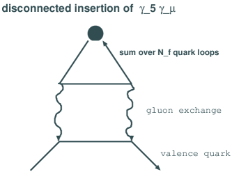
Figure 1: Perturbative triangle diagram of flavour singlet axial current as disconnected diagram with $\gamma_{5}\gamma_{\mu}$ insertion.

The lesson to be learnt is that pseudoscalar flavour singlet mesons are deeply affected by and thus indicative for the topological structure of the QCD vacuum. Needless to say that the time averaged vacuum expectation value of $Q=\tilde{Q}/(2N_{f})$ itself is zero, $\langle 0|Q(\vec{x})|0\rangle=0$, by translation invariance and parity conservation of strong interactions. As a consequence, the net topological charge of the QCD vacuum state is zero. The key quantity describing topological fluctuations of the QCD vacuum is the topological susceptibility, $\chi$, which is defined by

$$\chi=\int d^{4}x\langle 0|\,Q(x)Q(0)\,|0\rangle\;.$$ (5)

In the so-called ’t Hooft limit of the theory, when the number of colours, $N_{c}$ is taken to infinity ($N_{c}\rightarrow\infty$ at fixed value for the number of active flavours, $N_{f}$, in the weak gauge coupling limit $g^{2}\sim 1/N_{c}$), Witten and Veneziano were able to derive a simple relation for the $\eta^{\prime}$ mass in the chiral limit WV

$$m^{2}_{\eta^{\prime}}=\lim_{N_{c}\to\infty}\frac{2N_{f}}{F_{\pi}^{2}}\chi|_{quenched}\;,$$ (6)

where $F_{\pi}$ denotes the pion decay constant. Within the Witten-Veneziano model assumption, that the real world is well described by the above limit relation, LQCD can predict the $\eta^{\prime}$ mass by computing the topological susceptibility in quenched QCD.

The lattice implications of Eq. (6) have been discussed in quite some detail in a recent paper of GIUSTI et al lattice_WV . In this contribution we will focus on those problems that one encounters in the direct approach to extract physics from fermionic two-point correlators in the singlet sector.

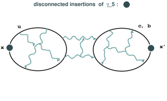
Figure 2: OZI rule violating quark fusion process with disconnected quark loops and $\gamma_{5}$ insertions.

2 Prolegomena: pseudoscalars in LQCD

In this section we shall consider a symmetric world with three flavours to enter the discussion on the computational tasks to be met.

2.1 Flavour octet sector

In the flavour octet sector of QCD (with mass degenerate $u,d,s$ quarks), the nonconservation of the axial vector current is determined by the PCAC relation:

$$\partial_{\mu}j_{5}^{\mu(8)}(x)=2m\bar{q}\gamma_{5}q\;,$$ (7)

which is much simpler in structure than its flavour singlet analogue, Eq. 3. In LQCD, the computation of the $\pi$-meson proceeds by hitting the vacuum state $|0\rangle$ with the quark bilinear pseudoscalar operator as given on the right hand side of Eq. (7). This creates both pions and excited $\pi$-like states. Let us consider such an operator carrying negative charge

$$\bar{u}(x)\gamma_{5}d(x)|0\rangle=|\pi^{-}\rangle_{x}+\mbox{ excited states}$$ (8)

with up and down quark operators, $u$ and $d$ respectively. The propagator in the pseudoscalar meson channel from $x$ to $x^{\prime}$, comprising the $\pi^{-}$-meson and its excited friends, would hence read like this:

$$G^{(8)}_{\mbox{PS}}(x,x^{\prime})=\langle 0|\bar{d}(x^{\prime})\gamma_{5}u(x^{\prime})\bar{u}(x)\gamma_{5}d(x)|0\rangle\;.$$ (9)

This vacuum expectation value is most easily computed by Wick contracting the two valence quark operators with matching flavour, and the result can be simply expressed in terms of the two quark propagators, $P_{u}=M_{u}^{-1}(x,x^{\prime})$ and $P_{d}=M_{d}^{-1}(x,x^{\prime})$ as follows:

$$G^{(8)}_{\mbox{PS}}(x,x^{\prime})=\mbox{Tr}[P^{*}_{u}(x,x^{\prime})P_{d}(x,x^{\prime})]\;,$$ (10)

where the trace is to be taken both in spin and colour space. In LQCD, the quark propagators (from source $x_{0}$ to sink $x^{\prime}$) can be computed in the background field of the QCD ground state (the vacuum) by solving the lattice Dirac equations

$$M_{D}(x^{\prime})P(x,x^{\prime})=\delta(x-x_{0})\;,$$ (11)

where $M_{D}$ is the discretized form of the Dirac operator including the gluon interaction and the r.h.s. denotes a point source located at lattice site $x_{0}$, see Fig. (3).

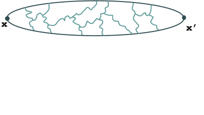
Figure 3: The connected propagator $G^{(8)}_{\mbox{PS}}(x,x^{\prime})$ for pseudoscalar meson states with negative charge, with a quark $d$ and an antiquark $\bar{u}$ running from source $x$ to sink $x^{\prime}$ in the unquenched QCD background field, with $\gamma_{5}$ insertions.

This is done by applying modern iterative solvers, like BiCGstab bicgstab . Note that

• $M_{D}\{U\}$ depends on the gluonic field configuration (i.e. the QCD vacuum configuration $\{U\}$ that has been produced independently by a suitable sampling process such as Hybrid Monte Carlo kennedy ; sesam )

• the efficiency of the solver is governed by the (fluctuating) condition number of the large sparse matrix $M_{D}\{U\}$ bicgstab ,ssor .

The simulation of the QCD vacuum on the lattice being a nonperturbative computation, the gluonic lattice vacuum configurations comprise the entirety of vacuum polarization effects, i.e. any conceivable fluctation from creation and annihilation of quarks and antiquarks (sea quark effects). So in Fig. (3) all vacuum polarization diagrams as depicted in Fig. (4) are understood to be included.

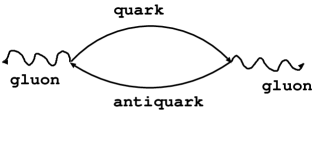
Figure 4: Gluon propagators including quark loop self energy diagrams.

We note in passing, that the numerical computation of the complete inverse of the lattice Dirac operator is prohibitively expensive: its computational effort grows with lattice volume, which in todays simulations is anywhere between $16^{4}$ and $64^{4}$ space-time lattice sites! So, in practical calculations of the $\pi$-meson, one restricts the source, $x_{0}$, to just a few space points in a particular time slice, say in $t=0$. The task for calculation is then the pseudoscalar two-point function:

$$G^{(8)}_{\mbox{PS}}(x_{0},x^{\prime})=\Big{<}\mbox{Tr}[P^{*}_{u}(x_{0},x^{\prime})P_{d}(x_{0},x^{\prime})]\Big{>}\;,$$ (12)

where the brackets denote the average over an ensemble of some hundred gauge field vacuum states. Note that it is enough in practice to compute but a few columns of the entire inverse Dirac matrix per configuration for achieving sufficient accuracy of the estimate, Eq. (12). Once this pseudoscalar two-point function has been calculated the pion contribution is obtained by removing the excited states from the pseudoscalar channel. For this purpose, one first extracts the zero momentum contributions by summing over all (spatial) $\vec{x}^{\prime}$ in time slice $t^{\prime}$:

$$C^{(8)}_{\mbox{PS}}(t=0,t^{\prime}):=\Big{<}\sum_{\vec{x}^{\prime}}\mbox{Tr}[P^{*}_{u}(x_{0},x^{\prime})P_{d}(x_{0},x^{\prime})]\Big{>}\;.$$ (13)

This latter two-point function at large enough time separations $t^{\prime}$ between source and sink will be dominated by the ground-state of the channel, i.e. the pion. Prior to that, it contains a superposition of ground and excited states:

$$C^{(8)}_{\mbox{PS}}(0,t^{\prime})=\sum_{i}c_{i}\exp(-E_{i}\,t^{\prime})\stackrel{{\scriptstyle t\rightarrow\infty}}{{\longrightarrow}}c_{0}\exp(-m_{\pi}t^{\prime})\;.$$ (14)

It is obvious that the strict localization of the source at the very lattice site $\vec{x}_{0}$ overly induces excited state contaminations; hence a suitable smearing of the source around this site will deemphasize such pollutions and will help to achieve precocious ground state dominance. This is welcome because the two-point correlator decreases exponentially and is prone to suffer large statistical fluctuations at large values of $t^{\prime}$.

The numerical task in exploiting Eq. (14) is then to optimize the smearing such as to achieve an early onset of a plateau: the latter is defined as the $t^{\prime}$-range over which $G^{(8)}_{\mbox{PS}}(0,t^{\prime})$ decays with a single exponential. This is tantamount to requiring the ’local pseudoscalar mass’, $m_{\mbox{PS}}(t^{\prime})$, to remain constant:

$$m_{\mbox{PS}}(t^{\prime}):=-\partial_{t^{\prime}}ln[C^{(8)}_{\mbox{PS}}(0,t^{\prime})]\stackrel{{\scriptstyle!}}{{=}}\mbox{const.}=m_{\pi}\;.$$ (15)

Smearing of sources or sinks is achieved by a diffusive iteration sesam process: think of replacing pointlike sources or sinks by

$$\delta(x_{0})=\phi^{(0)}(x_{0})\longrightarrow\phi^{(N+1)}(x)\;,$$ (16)

where $\phi^{(N)}(x)$ is peaked around $x_{0}$ and is constructed by the recursion

$$\phi_{s}^{(i+1)}(x)=\frac{1}{1+6\alpha}\left[\phi_{s}^{(i)}(x,t)+\alpha\sum_{\mu}\phi_{s}^{(i)}(x+\mu)^{\mbox{{\tiny p.t.}}}\right]\;.$$ (17)

The index ‘p.t.’ stands for ‘parallel transported’, and the sum extends over the six spatial neighbours of $x$. As a result the entire series of smeared ’wave functions’ $\phi^{(i)},i=1,2,\cdots,N-1$ is gauge covariant under local gauge transformations. Quark operators are computed after $N=25$ such smearing steps, with the value $\alpha=4.0$. The smearing procedure is applied to meson sources as well as to sinks for connected and disconnected diagrams.

2.2 Flavour singlet sector

In the case of $SU(3)$ flavour symmetry the appropriately normalized flavour singlet pseudoscalar operator reads

$$O^{(0)}(x)=\frac{1}{\sqrt{3}}\sum_{i}\bar{q}_{i}(x)\gamma_{5}q_{i}(x)\;.$$ (18)

Here the sum extends now equally over all (mass degenerate $u$, $d$, and $s$) quark flavours. The flavour singlet pseudoscalar meson propagator is estimated from the average

$$G^{(0)}_{\mbox{PS}}(x,x^{\prime})=\Big{<}O^{(0)\dagger}(x^{\prime})O^{(0)}(x)\Big{>}\;.$$ (19)

In this case the Wick contraction now induces both connected and disconnected (two-loop) diagrams, $D$,

$$D(x,x^{\prime})=\Big{<}\mbox{tr}[O^{(0)\dagger}(x^{\prime})]\mbox{tr}[O^{(0)}(x)]\Big{>}\;,$$ (20)

such that finally

$$G^{(0)}_{\mbox{PS}}(x,x^{\prime})=G^{(8)}_{\mbox{PS}}(x,x^{\prime})-N_{f}D(x,x^{\prime})\;,$$ (21)

as depicted in Fig. (5). Note that at this stage the trace operations in Eq. (20) refer to spin and colour space only and the Wick contraction procedure leads to the weight $N_{f}=3$ of the disconnected relative to the connected contribution, the latter being identical to the expression given in Eq. (13). The relative minus sign is due to Fermi statistics of the quark operators.

We note in passing, that connected and disconnected correlators come along with intrinsic positive sign such that the above minus sign leads to a steepening of $C^{(0)}(t^{\prime})$ w.r.t. $C^{(8)}(t^{\prime})$, iff $D$ shows a soft drop in $t^{\prime}$.

Figure 5: The connected and OZI-rule violating (’disconnected’) contributions to the $\eta^{\prime}$ propagator $G_{\mbox{PS}}^{(0)}$ from Eq. (19). Note that these diagrams keep only track of the valence quark lines: all gluon exchanges due to the vacuum background field have been omitted for clarity of the graph. It goes without saying that in unquenched QCD, the gluon propagators implicitly induce sea quark loops as in Fig. (4).

Let us mention that the terminology “two-loop correlator” might be misleading: it refers to the fact that we are dealing here with two (valence quark) loop insertions of the $\gamma_{5}$ operator. The unquenched QCD vacuum includes of course a host of sea quark loops that are implicitely taken into account when sampling unquenchced QCD vacua in a LQCD simulation. They would enter in form of vacuum polarization effects on the very gluon propagators as depicted in Fig. (4).

Figure 6: Pictorial receipe for setting up the $\eta^{\prime}s$ propagator in quenched QCD as an explicit multiloop expansion.

It is illuminating to consider the mechanism for the origin of the singlet octet mass gap in a model to real QCD: let us start in the $N_{c}=\infty$ world, where the $U_{A}(1)$ symmetry holds and flavour octet and singlet mesons are degenerate, $m_{0}=m_{8}$. This degeneracy is only broken by the higher quark loop contributions which are suppressed by inverse powers in $N_{c}$. It is hence straightforward to approximate the $\eta^{\prime}$ propagator, starting out from this scenario, as an explicit multiloop expansion of quark antiquark annihilation diagrams in the pure gluonic background field of quenched QCD, as illustrated in Fig. (6). The actual calculation can be greatly simplified by introducing an effective loop-loop coupling, $\mu_{0}^{2}$. In momentum space the $\eta^{\prime}$-propagator then takes the form of a geometric series:

$$P_{\eta^{\prime}}=\frac{1}{p^{2}+m_{8}^{2}}\Bigg{(}1+\sum_{l=1}^{\infty}\bigg{[}\frac{-\mu_{0}^{2}}{p^{2}+m_{8}^{2}}\bigg{]}^{l}\;\Bigg{)}\;.$$ (22)

The series is readily summed up with the result:

$$P_{\eta^{\prime}}=\frac{1}{p^{2}+(m_{8}^{2}+\mu_{0}^{2})}\;,$$ (23)

which reveals that the effective loop-loop coupling is nothing but the mass gap between singlet and octet pseudoscalar masses:

$$\Delta m^{2}=:m_{0}^{2}-m_{8}^{2}=\mu_{0}^{2},$$ (24)

We emphasize that in this effective model it is only by summation of the entire series to all orders in $l$ that we arrive at a simple pole expression for the singlet propagator in momentum space and hence at a simple exponential falloff in time of the two-point correlator. Note that this summation happens automatically in an unquenched QCD situation where all multiquarkloop effects are already implicitly included in the very gauge field vacuum configuration!

3 The real world with $n\bar{n}$ $s\bar{s}$ mixing

So far we have been leading a rather academic discussion in an SU(3) symmetric world. We would like next to describe the $\eta$/$\eta^{\prime}$ problem in a more realistic setting. This opens up a pandora box of four parameters for decay matrix elements plus the mixing angle among isosinglet particle states. Two degrees of freedom in the decay constants can be characterized as mixing angles leutwyler .

3.1 Phenomenological approach: alignment hypothesis

In order to ease the interpretation of flavour breaking effects in the isosinglet sector, Feldmann et al fks ; kroll have proposed some time ago an intuitive scheme to describe the $\eta-\eta^{\prime}$ phenomenology by use of a quark state Fock state representation in conjunction with an alignment assumption. The latter reduces the number of parameters to two couplings plus a single mixing angle of the particle states in that Fock space. Let us briefly review their scenario: they proceed from the two isosinglet states

$$|\eta_{n}\rangle = \Psi_{n}|u\bar{u}+d\bar{d}\rangle/\sqrt{2}+\dots$$ (25)

$$|\eta_{s}\rangle = \Psi_{s}|s\bar{s}\rangle+\dots\quad,$$ (26)

where $\psi_{n,s}$ denote light cone wave functions . The key assumption of their phenomenological approach is their hypothesis of alignment of the current matrix elements:

$$\langle 0|\bar{q}_{i}\gamma_{5}\gamma_{\mu}q_{i}|\eta_{j}\rangle=\delta_{ij}f^{i}p_{\mu}\;,i,j=n,s\;.$$ (27)

Due to the QCD interactions the physical $\eta$ and $\eta^{\prime}$ states will turn out to be mixtures of these Fock states:

$$\left(\begin{array}[]{c}|\eta\rangle\\ |\eta^{\prime}\rangle\end{array}\right)=U(\phi)\left(\begin{array}[]{c}|\eta_{n}\rangle\\ |\eta_{s}\rangle\end{array}\right):=\left(\begin{array}[]{cc}\cos\phi&-\sin\phi\\ \sin\phi&\cos\phi\end{array}\right)\left(\begin{array}[]{c}|\eta_{n}\rangle\\ |\eta_{s}\rangle\end{array}\right)\;.$$ (36)

As a consequence of the alignment hypothesis, Eq. (27), the four decay constants, $f^{i}_{P}$

$$\langle 0|j_{\mu 5}^{i}|P\rangle=\langle 0|\bar{q}_{i}\gamma_{5}\gamma_{\mu}q_{i}|P\rangle\equiv f^{i}_{P}p_{\mu}\quad i=n,s;\quad P=\eta,\eta^{\prime}$$ (37)

can be expressed in terms of $f^{n},f^{s}$ and the very rotation angle $\phi$ fks :

$$\left(\begin{array}[]{cc}f^{n}_{\eta}&f^{s}_{\eta}\\ f^{n}_{\eta^{\prime}}&f^{s}_{\eta^{\prime}}\end{array}\right)=U(\phi)\left(\begin{array}[]{cc}f^{n}&0\\ 0&f^{s}\end{array}\right)\;.$$ (42)

By feeding the anomalous PCAC relation

$$\partial^{\mu}\bar{q}_{i}\gamma_{5}\gamma_{\mu}q_{i}=2m_{i}\bar{q}_{i}\gamma_{5}q_{i}+\tilde{Q}$$ (43)

into the four decay matrix elements

$$\langle 0|\partial^{\mu}j_{\mu 5}^{i}|\eta\rangle=f^{i}_{\eta}m_{\eta}^{2},\quad\langle 0|\partial^{\mu}j_{\mu 5}^{i}|\eta^{\prime}\rangle=f^{i}_{\eta^{\prime}}m_{\eta^{\prime}}^{2};\quad(i=n,s)\;,$$ (44)

the authors of ref.fks ; kroll ; feldmann arrive at the mass matrix mixing relation

$$\left(\begin{array}[]{cc}\mu_{nn}^{2}+\frac{\sqrt{2}}{f^{n}}\langle 0|\tilde{Q}|\eta_{n}\rangle&\frac{1}{f^{s}}\langle 0|\tilde{Q}|\eta_{n}\rangle\\ \frac{\sqrt{2}}{f^{n}}\langle 0|\tilde{Q}|\eta_{s}\rangle&\mu_{ss^{2}}+\frac{1}{f^{s}}\langle 0|\tilde{Q}|\eta_{s}\rangle\\ \end{array}\right)=U^{\dagger}(\phi)\left(\begin{array}[]{cc}m^{2}_{\eta}&0\\ 0&m^{2}_{\eta^{\prime}}\end{array}\right)U(\phi)\;,$$ (49)

with a single mixing angle that is in accord with Fock state mixing. In Eq. (49) the abbreviations $\mu^{2}$ stand for the explicit chiral symmetry breaking terms from nonvanishing quark masses, $m_{i}$:

$$\mu_{ii}^{2}:=\frac{2m_{i}}{f_{n}}\langle 0|\bar{q_{i}}\gamma_{5}q_{i}|\eta_{i}\rangle;\quad i=n,s\;.$$ (50)

For consistency of the approach, they have to postulate the symmetry of the mass matrix, which sets a constraint among the matrix elements $\langle 0|\tilde{Q}|\eta_{i}\rangle;\;i=n,s\;.$

The l.h.s. of Eq. (49) being a continuum relation, great care must be exercised in renormalizing the operators. Since the underlying anomalous PCAC relation, Eq. (43) is actually to be seen as a Ward-Takahashi identity from chiral rotations, the standard Wilson lattice fermions provide a problematical scheme for regularizing the matrix entries in Eq. (49), with the Wilson lattice fermions lacking chiral symmetry at finite lattice spacing bochiccio . This complex situation would be largely improved when dealing with Ginsparg-Wilson fermions in unquenched QCD, whose lattice chiral symmetry prevents undesired divergencies from operator mixings lattice_WV . On the lattice, the mass² entries to the matrix Eq. (49) are best accessible from propagator studies in the singlet channels kilcup ; ukqcd ; michael ; michael_rev .

We would like to explain next, that the idea of Fock state mixing of eigenstates can in principle be pursued very naturally from a variational approach on the lattice, once we have fully unquenched QCD vacuum configurations in the future, without making reference to an alignment hypothesis.

3.2 Mixing singlet mesons on the lattice

On the lattice, we can prepare the the Fock states $|\eta_{n}\rangle$ and $|\eta_{s}\rangle$ by hitting the vacuum at some (smeared) source location, say $x=(0,0,0,0)$, with the bilinear isosinglet operators,

$${\cal O}_{i}(0)|0\rangle=\bar{q}_{i}(0)\gamma_{5}q_{i}(0)|0\rangle,\quad i=n,s$$ (51)

and by waiting long enough to see the ground states emerge.

In the sense of a variational method, one can next work with a superposition of these operators to achieve earlier exponential decay of the correlator and/or lowering of the ground state, the $\eta$-meson:

$${\cal O}_{\alpha}=\cos\alpha\;{\cal O}_{n}-\sin\alpha\;{\cal O}_{s}\;.$$ (52)

Suppose this variational ansatz delivers an immediate plateau for some value of the variational parameter, $\alpha=\alpha^{*}$: in that case we have actually hit an eigenmode of the interacting system and the Fock state mixing angle is $\phi=\alpha^{*}$! Since one expects little mixing with higher Fock states, one could then recover the $\eta^{\prime}$ ground state from the orthogonal combination

$${\cal O}_{\alpha}^{\perp}=\sin\alpha\;{\cal O}_{n}+\cos\alpha\;{\cal O}_{s}\;.$$ (53)

In general the state mixing information is encoded more deeply in the correlation matrix (still in operator quark content basis)

$${\cal C}(t)=\left(\begin{array}[]{cc}C_{nn}(t)-2D_{nn}(t)&\sqrt{2}D_{ns}(t)\\ \sqrt{2}D_{sn}(t)&C_{ss}(t)-D_{ss}(t)\end{array}\right)\;.$$ (56)

Note that the weight factors $2$ and $\sqrt{2}$ in this relation originate from the combinatorics when Wick contracting the degenerate $u$ (with $\bar{u}$) and $d$ (with $\bar{d}$) quark operators contained ${\cal O}_{n}$

$$\bar{q}_{i}\gamma_{5}q_{n}:=\frac{1}{\sqrt{2}}(\bar{u}\gamma_{5}u+\bar{d}\gamma_{5}d)\;.$$ (57)

If plateau formation does not occur immediatley, at $t_{p}=0$, one needs to follow the time evolution up to a later time step when the higher excitations have died out, and ascertain the plateau condition within the time interval $t_{p}\rightarrow t_{p}+\Delta t$ in form of a generalized eigenvalue problem wolff :

$${\cal C}(t_{p}+\Delta t)\left(\begin{array}[]{c}+\cos\alpha\\ -\sin\alpha\end{array}\right)=\exp(-m_{\eta}\Delta t)\;\;{\cal C}(t_{p})\left(\begin{array}[]{c}+\cos\alpha\\ -\sin\alpha\end{array}\right)\;.$$ (62)

The problem can be recast into a symmetric form

$${\cal C}^{-1/2}(t_{p}){\cal C}(t_{p}+\Delta t){\cal C}^{-1/2}(t_{p})\cdot\vec{\eta_{\alpha}}=\exp(-m_{\eta}\Delta t)\cdot\vec{\eta_{\alpha}}\;$$ (63)

with the definition

$$\vec{\eta_{\alpha}}(t_{p})={\cal C}^{+1/2}(t_{p})\left(\begin{array}[]{c}+\cos\alpha\\ -\sin\alpha\end{array}\right)$$ (66)

According to the symmetric plateau condition, Eq. (63), the direction of the ground state vector, $\vec{\eta_{\alpha}}(t_{p})$, remains fixed under further time displacements $\Delta t$ through the transfer operator, ${\cal T}(\Delta t)={\cal C}^{-1/2}(t_{p}){\cal C}(t_{p}+\Delta t){\cal C}^{-1/2}(t_{p})$. Hence the $\eta$ mixing angle in the quark state basis is given by the direction of eigenvector $\vec{\eta_{\alpha}}(t_{p})$ at the onset of the plateau and might differ appreciably from the variational angle $\alpha$. The problem Eq. (63) being symmetric, the $\eta^{\prime}$ is retrieved as the second, perpendicular eigenstate of ${\cal T}(\Delta t)$.

It might be illuminating to put Eq. (63) into perspective with the previous plateau condition, Eq. (15): by Taylor expanding of ${\cal C}(t_{p}+\Delta t)$ to lowest order in $\Delta t$ one can readily recast Eq. (63) into a local condition, with a ’logarithmic derivative’ matrix construct, ${\cal C}^{-1/2}(t_{p}){\cal C}^{\prime}(t_{p}){\cal C}^{-1/2}(t_{p})$:

$${\cal C}^{-1/2}(t_{p}){\cal C}^{\prime}(t_{p}){\cal C}^{-1/2}(t_{p})\cdot\vec{\eta_{\alpha}}(t_{p})=-m_{\eta}\cdot\vec{\eta_{\alpha}}(t_{p})\;.$$ (67)

In principle, the phenomenological alignment postulate of Eq. (27) can be tested on the lattice by computing another, nonsymmetric set of correlators

$$\tilde{{\cal C}}_{ij}(t)=\langle 0|\partial^{\mu}\bar{q}_{i}(t)\gamma_{5}\gamma_{\mu}q_{i}(t)\bar{q}_{j}(0)\gamma_{5}q_{j}(0)|0\rangle\;,$$ (68)

which allows to extract the various decay matrix elements. Let us emphasize in concluding this section that the scenario presented here relates to fully unquenched three flavour QCD; according to the discussion in 2.2 the mass plateau conditions can only be anticipated if the quark contents of the bilinear operators in Eq. (51) are equally present in the quark sea .

4 The three computational bottlenecks

In this section we shall focus in more detail on the numerical obstacles that one encounters when carrying out the above program. These difficulties are computationally much more severe than in nonsinglet spectroscopy and hence require the development of advanced algorithms and numerical techniques:

1. Present limitations in sea quark flavours. It was only in the second half of the nineties that LQCD had developed the means to tackle first semi-realistic large scale simulations of QCD beyond the valence (or ‘quenched’) approximation. The reason is that Wilson-like discretizations of the Dirac operator are mandatory once we wish to deal with strong interaction situations sensitive to flavour symmetry. But such Wilson-like lattice fermions need extremely large supercomputer resources when it comes to actually simulate the effects of dynamical sea quarks, i.e. to sample unquenched CCD vacuum configurations. The hybrid Monte Carlo algorithm (HMC) is a nonlocal sampling technique which was developed and improved ever since the late eighties kennedy ; it continues to be the workhorse in all of the major QCD simulation projects with Wilson-like fermions sesam ; cppacs ; ukqcd ; qcdsf . For technical reasons, however, HMC has the shortcoming of being limited to even numbers of sea quark flavours. As a consequence, all the above projects neglected dynamical $s$-quarks in working with mass degenerate $u$ and $d$ sea quarks only, i.e. considered an $SU(2)$ symmetric sea of quarks only. It is to be hoped that the next generation of large-scale QCD simulation with Teracomputers will overcome this limitation with new sampling algorithms.

2. Trace computations. We have seen that the peculiarity of flavour singlet objects lies in the annihilation of the valence quark lines into the flavour blind gluonic soup which implies the need to compute disconnected diagrams. But inspection of Eq. (20) shows that the $\vec{x^{\prime}}$-summation from momentum zero projection requires the evaluation of the trace of the inverse Dirac operator. This task is definitely beyond the reach of modern linear equation solvers for matrices of rank $10^{6}$ and more. Traditionally stochastic estimator techniques (SET) have been the popular workaround stoch ; struckmann .

3. Noisy signals.

The singlet spectrum being inherently determined by the physics of the quantum fluctuations of the QCD vacuum, the two-loop correlators are bound to suffer from a serious noise level. This calls for the use of noise reduction methods, in order to circumvent the need for overly large ensembles of vacuum field configurations. With this motivation low mode expansion methods have been proposed recently with considerable success to replace stochastic estimator techniqueskilcup ; tea .

4.1 Stochastic estimate of fermion loops

The basic idea of stochastic estimation of the momentunm zero projected loop operator in Eq. (20), $\sum_{\vec{x}}\mbox{tr}\big{(}\gamma_{5}M^{-1}(\vec{x},t)\big{)}$, is very simple: instead of attempting to solve Eq. (11) $V$ on delta-like sources, one introduces socalled stochastic volume sources which are completely delocalized, on the entire lattice volume V:

$$\xi=(\xi_{1},\xi_{2},\dots,\xi_{V})\;.$$ (69)

The components $x_{i}$ are chosen to be real random numbers sampled from a normal distribution $N(x_{i})=1/\sqrt{2\pi}\exp(-x_{i}^{2}/2)$ or socalled $Z_{2}$ noise which is nothing but equally distributed random numbers $\pm 1$. One solves the Dirac lattice equation on an ensemble of $N_{s}$ such random source vectors, $\{\xi^{\alpha}\}$, for each individual gauge configuration:

$$\zeta^{\alpha}=\gamma_{5}M_{D}^{-1}\xi^{\alpha}\;.$$ (70)

and computes the ensemble average of the scalar products

$$\Big{<}(\xi,\zeta)\Big{>}_{s}\;:=\;\frac{1}{N_{s}V}\sum_{\alpha=1}^{N_{s}}\sum_{i=1}^{V}\xi^{*\alpha}_{i}\zeta^{\alpha}_{i}\simeq\mbox{TR}\Big{[}\gamma_{5}M_{D}^{-1}\Big{]}\;.$$ (71)

One might phrase this procedure as an all-at-one-stroke method, at the expense of nonclosed loops sneaking in, in form of contributions from $\Big{[}\gamma_{5}M_{D}^{-1}\Big{]}_{ij}$ with $i\neq j$. These undesired contributions are suppressed, however, due to the ’componentwise orthonormality’ relation

$$\Big{<}\xi_{i}^{*}\xi_{j}\Big{>}_{s}=\frac{1}{N_{s}}\sum_{\alpha=1}^{N_{s}}\xi^{*\alpha}_{i}\xi^{\alpha}_{j}\stackrel{{\scriptstyle N_{s}\rightarrow\infty}}{{\longrightarrow}}\delta_{ij}\;.$$ (72)

Note that Eq. (71) readily allows for restricting the grand trace operation over the entire space-time lattice, TR, to any particular time slice, simply by truncating the $i$-summation to the appropriate three-dimensional subvolume, such as to yield the estimator for the momentum zero expression on time slice $t$, $\sum_{\vec{x}}\mbox{tr}\big{(}\gamma_{5}M^{-1}(\vec{x},t)\big{)}$.

In principle, these considerations hold for all kinds of insertions, not just $\gamma_{5}$ like in our example. In any case the ’sneakers’ are suppressed as ${\cal O}(N_{s}^{-1})$ terms, but with a strength that depends on the insertion. The practical advantage of this stochastic procedure is, that in the instance of $\gamma_{5}$ insertions one needs to compute only some few hundred solutions to Eq. (70) which is much less than ${\cal O}(V)$! But we should keep in mind that this is achieved only at the expense of injecting additional noise into the problem.

4.2 Low eigenmode approximation to fermion loops

We start with the eigenvalue problem for the socalled Hermitian Dirac operator,

$$Q_{5}:=\gamma_{5}M_{D}\;,$$ (73)

which reads

$$Q_{5}\psi_{i}=\lambda_{i}\psi_{i}\;.$$ (74)

The quark loop with $\gamma_{5}$ insertion at time slice $t$ is simply expressed in terms of this eigensystem:

$$Q_{5}^{-1}(t)=\sum_{i}\frac{1}{\lambda_{i}}\frac{\langle\psi_{i}(t)|\psi_{i}(t)\rangle}{\langle\psi_{i}|\psi_{i}\rangle}\;.$$ (75)

The disconnected two-loop correlator from Fig. (5) then has the form

$$D(t)=\sum_{t_{0}}\sum_{i}\frac{1}{\lambda_{i}}\frac{\langle\psi_{i}(t_{0})|\psi_{i}(t_{0})\rangle}{\langle\psi_{i}|\psi_{i}\rangle}\sum_{j}\frac{1}{\lambda_{j}}\frac{\langle\psi_{j}(t_{0}+t)|\psi_{j}(t_{0}+t)\rangle}{\langle\psi_{j}|\psi_{j}\rangle}\;,$$ (76)

where $t$ represents the time separation between source and sink and we have exploited translational invariance by summing over all time locations of the source, $t_{0}$. This summation is for free, once the eigenfunctions are available. The determination of the entire spectrum being of course prohibitively expensive, we proceed by arranging the spectrum in ascending order of $|\lambda_{i}|$ attempting to saturate the eigenmode expansion, Eq. (76), with its lowest modes. The intuitive reasoning behind such a strategy is, that the underlying physics is expected to be encoded in the infrared rather than ultraviolet modes. After all, it is well known that for Wilson fermions 15/16 of the spectrum is related to the unphysical doublers that become frozen to order ${\cal O}(a^{-1})$ as the lattice spacing $a$ is going to zero.

Figure 7: Cumulative spectral distribution of the lowest eigenmodes at the smallest (lower curve) and largest (upper curve) sea quark masses of the SESAM project tea .

Fig. (7) offers an impression on the cumulative distribution of the lowest modes of the Dirac operator in the situation of the SESAM simulation, at their smallest and largest sea quark masses. Note that the masses of valence quarks (inserted into the Dirac operator) and sea quarks (inserted into the hybrid Monte Carlo sampling of gauge field configurations) are chosen to coincide; Fig. (7) therefore reflects the feedback mechanism from dynamical effects onto the spectral representation as quark masses are diminished. Fig. (7) suggests that the important spectral activity is mostly within the lowest 50 modes.

But how many modes do suffice for saturating Eq. (76)?

Figure 8: Pion correlator in spectral approximation, plotted versus spectral cutoff, $\lambda_{c}$. Shown is a sequence of trajectories, as obtained on fixed values of $t$: the curves represent $C^{(8)}(t=1)$, $C^{(8)}(t=2)$, $C^{(8)}(t=3)$ etc , from top to bottom tea . In this representation the justification of truncation is signaled by a flat $\lambda_{c}$-dependency.

For the saturation of the two point correlators, one would anticipate the need for larger values for the cutoff, $\lambda^{c}$, as one diminishes the time separations towards a few lattice spacings. This expectation is indeed confirmed by the numerical results for the pion corrrelator as displayed in Fig. (8): The diagram shows a sequence of curves which – in descendig order – refer to $C(t=1),C(t=2),\cdots,C(t=16)$, which are plotted versus the spectral cutoff. For small values of $t$ the curves keep rising with $\lambda_{c}$, while asymptotic saturation is found to be better at larger $t$-values.

In Fig. (9), we plotted the pion correlator from a truncated eigenmode approximation (TEA) with cutoff $\lambda_{c}=300$ and from standard iterative solvers. There remain noticeable differences in the two curves for this value of the cutoff. Therefore, one would refrain from using TEA for connected hadron propagators unless really needed. The situation w.r.t. $\lambda^{c}$ turns out to be much more favourable with the disconnected piece, $D(t)$, as shown in Fig. (10).

Figure 9: Quality of the truncated eigenmode approximation at the smalles SESAM sea quark mass for the pion correlator, with a spectral cutoff, $\lambda_{c}=300$. Satisfactory agreement with the standard result from using iterative solvers is only reached at $t\simeq 10$.

How well the idea of saturation actually works out quantitatively is illustrated in Fig. (11), where we compare the two-loop correlator in the truncated eigenmode approximation (TEA) against the results from a previous comprehensive study with the estimation by an ensemble of stochastic sources struckmann . We find that the contributions from the lowest 300 eigenmodes agree remarkably well with the SET computations which are based here on 400 source vectors, on a $16^{\times}32$ lattice in the sea quark mass range covered used by the SESAM project! The net computational effort behind the two sets of data points in Fig. (11) is about equal, yet the TEA data among themselvesa appear to be less fluctuating.

Figure 10: Quality of low eigenmode approximation as function of time separation for the OZI rule violating term, $D(t)$. The curves represent (from top to bottom) $C(1),C(2),\cdots,C(16)$ tea .

This positive message from Fig. (11) bears substantial promise for future lattice studies with lighter quark masses, as SET is doomed to degrade when penetrating more deeply into the more chiral regime while the truncated eigenmode approximation (TEA) will thrive: (a) the lowest modes will dominate all the more as $|\lambda_{min}|$ approaches zero; (b) modern Arnoldi eigensolvers have been made very efficient in present day LQCD simulations neff_solver and will not deteriorate for lighter quarks as long as one sticks to fixed lattice volumes. Conversely, iterative solvers on stochastic sources will suffer substantial losses in convergence rate, once the condition number of the Dirac matrix, $c:=|\lambda_{max}/\lambda_{min}|$ starts exploding.

Figure 11: The two-loop correlator, $D(\Delta t)$, as obtained from SET struckmann (circles) and TEA (triangles) in comparison. Local sources and sinks have been used and $N_{s}=300$ and $\lambda_{c}=300$ were chosen tea .

4.3 Navigating between Scylla and Charybdis

There is another lesson from Fig. (11): we find the noise level in $D(t)$ to be rather independent of $t$, i.e. of signal size. This is of course in line with the fact that we are hunting for vacuum fluctuations proper. It therefore appears impracticable to achieve ground state projection in the very standard fashion by increasing $t$: the $\eta^{\prime}$ correlator being the imbalance between connected and two-loop signals one is to keep track of a signal in form of a rapidly diminishing difference between two quantities, with one being at fixed noise level. Given this situation we are challenged by complying to two conflicting needs: on one hand large $t$ values are needed to deflate excited state contaminations and on the other hand the struggle for an acceptable signal-to-noise ratio impedes working in the large-$t$ regime. Our strategy to deal with this conundrum of the $\eta^{\prime}$ correlator, Eq. (21) is to contrive a procedure for circumventing this conflicting requirements. The receipe is the following:

• suppress the excited states from $C_{PS}^{(8)}(\Delta t)$ by using an exponential fit from the window of its mass plateau;

• deemphasize the short range noise level inside $D$ by means of the truncated eigenmode expansion, Eq. (76).

This method could also be characterized through an intermediate ’synthetic data stage’ since the actual ground state analysis for the singlet correlator is organized as a sequence of three steps:

(a) extract

an exponential fit to the lattice data for $E(\Delta t)=C_{PS}^{(8)}(\Delta t)$,

(b) combine

this fit curve, $E(\Delta t)$, with the lattice data for $D(\Delta t)$ into the ’synthetic’ data set for $C_{PS}^{(0)}(\Delta t):=E(\Delta t)-N_{f}D(\Delta t)$, in the spirit of Eq. (21),

(c) establish

a mass plateau in $C_{PS}^{(0)}(\Delta t)$ and perform another exponential fit to $C_{PS}^{(0)}(\Delta t)$ within the plateau region in order to determine the singlet pseudoscalar mass.

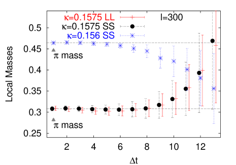
Figure 12: Mass plateau formation in the $\eta^{\prime}$ (singlet) correlator after dual filtering with TEA, for two different values of hopping parameters (sea quark masses) versus time separation between source and sink, $\Delta t$ tea . The plot shows the respective lattice values for the pion (nonsinglet) mass for comparison. The effect of smearing onto the signal is also illustrated: SS and LL refer ’to smeared source and sink’ and ’local source and sink’, respectively.

We find this dual filtering approach to operate very well in the two-flavour case, on the SESAM QCD configurations. This is illustrated in Fig. (12) which manifests very clearly a plateau in the local mass plot of the $\eta^{\prime}$-correlator. The onset of plateau formation is precocious in the sense that we still maintain very precise signals. Therefore the statistical accuracy is sufficiently high to resolve the mass gap between the singlet and nonsinglet masses, whose lattice values for these sea quark masses are also included in the plot, being indicated with the symbol ’$\pi$’.

Let us emphasize that we consider the upshot of precocious asymptotia in the $\eta^{\prime}$-correlator as an essential outcome of our analysis; it corroborates that the nonperturbative lattice simulations take effect in implicitly creating the mass gap between singlet and nonsinglet states, much in line with the perturbative reasoning from Eq. (22): indeed, the simulation data for the two-loop correlator, $D(t)$, turn out to be the difference between just two exponentials rather than a multiexponential superposition. This will enable us to perform a rather detailed physics analysis in the singlet pseudoscalar channel.

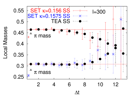
Figure 13: Comparing mass plateaus of the singlet correlator obtained with SET and TEA tea . Smeared sources and sinks are used throughout. Notations as in Fig. 12.

One might still worry about possible systematic errors from spectral truncation in the singlet mass plateaus contained in Fig. (12). In this context it is reassuring to observe nice agreement within errors with the results obtained from stochastic sources, as illustrated in Fig. (13).

It is interesting to compare the plateau formation from dual filtering (Fig. (12)) with the state-of-the-art results from optimized smearing as obtained in the most recent comprehensive studies of the CP-PACS collaboration cppacs (Fig. (14)). The comparison teaches us that dual filtering is indeed remarkably effective in unravelling the mass plateaus in the pseudoscalar singlet mesons.

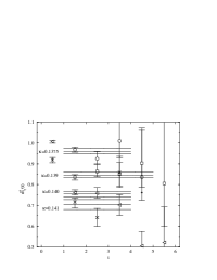
Figure 14: State-of-the-art mass plateau formation from optimized smearing as obtained in a comprehensive study by the CP-PACS group, at their smallest lattice spacing, $a=.1076$ fm, on a $24^{3}\times 48$ lattice, for various sea quark masses. Quotation from Ref. cppacs .

5 Towards realistic physics results

5.1 Unquenched two flavour world

Given the good quality of signals within the SESAM setting, we are prepared to compute the entire mass trajectory of singlet pseudoscalars. In table 1 we list the essential run parameters of the SESAM project, which is based on vacuum field configurations from standard Wilson fermions on a $16^{3}\times 32$ lattice sesam , with two active sea quark flavours, at one value of the coupling, $\beta=5.6$. Four different sea quark masses have been used. The most interesting control parameter is the ratio between the pion and $\rho$-meson masses as determined on the lattice; it is quoted in the second column of table 1.

Table 1: Simulation parameters used at $\beta=5.6$ and numbers of stochastic sources $N_{s}$ (see Eq.  71 and Fig.  13). Last column: numbers of available decorrelated vacuum field configurations, $N_{conf}$.

$\kappa_{sea}$	$m_{\pi}/m_{\rho}$	$L^{3}*T$	$N_{s}$	$N_{conf}$
0.1560	0.834(3)	$16^{3}*32$	$400$	$195$
0.1565	0.813(9)	$16^{3}*32$	$400$	$195$
0.1570	0.763(6)	$16^{3}*32$	$400$	$195$
0.1575	0.692(10)	$16^{3}*32$	$400$	$195$

This setting allows for a chiral mass extrapolation of the singlet pseudoscalar meson composed of $u$ and $d$ quarks, as plotted in Fig. (15). The plot contains the mass trajectory for the singlet channel as well as the nonsinglet extrapolation, marked by ’$\pi$’. We conclude that the data allow for a safe chiral extrapolation in both channels, though there is definite need to lower the sea quark masses in the simulations. The precision is sufficient to resolve the mass gap between singlet and nonsinglet pseudoscalars.

As we have excluded strange quarks altogether, we can of course not expect to hit the experimental $\eta^{\prime}$ mass: the extrapolated singlet mass of $290$ MeV should be compared to the $\eta$ rather than to the $\eta^{\prime}$ mass. It is evident, that we must address the issue of treating strange quarks in addtion to $u$ and $d$ quarks.

Figure 15: Plot of $m_{\eta}^{2}$ versus quark mass, all given in lattice units neff_boston .

Another shortcoming of SESAM is its restriction to one coupling $\beta$ which does not allow for a continuum extrapolation. Very recently, the CP-PACS collaboration has found in their $N_{f}=2$ study with an improved action that this extrapolation tends to induce a considerable increase in the pseudoscalar singlet mass cppacs .

5.2 Partially quenched scenario for the three flavour world

One of the main restrictions of todays unquenched QCD simulations is their limitation to two mass degenerate dynamical sea quark flavours. This presents a serious shortcoming when dealing with the real physics of the $\eta$-$\eta^{\prime}$ system. Nevertheless, the partially quenched approach part_quen offers a crutch to include the strange quark sector into the analysis. In the partially quenched scenario, strange quarks might appear as valence quarks only and not contribute at all dynamically to the quark sea.

For the sake of discussion, let us depart from the fully quenched situation. In this setting, the $s$-loop $s$-loop correlator, $D_{ss}$ in Eq. (56), amounts to the occurence of a double-pole:

$$m_{0,ss}^{2}/(p^{2}+m_{s}^{2})^{2}$$

in momentum space. In this expression, $m_{s}$ denotes the valence approximation mass estimate for the pseudoscalar $\bar{s}s$ meson that can be determined on the lattice from the connected piece of the $C_{ss}$ correlator. As we have seen in section 2.2, the double pole impedes an exponential decay in $t$ and hence will require a different strategy of analysis: it can readily be rewritten as a derivative on the single pole expression

$$m_{0,ss}^{2}/(p^{2}+m_{s}^{2})^{2}=-\frac{\partial}{\partial m_{s}^{2}}\;\frac{m_{0,ss}^{2}}{p^{2}+m_{s}^{2}}\;.$$ (77)

Iff $m_{0,ss}^{2}$ is a constant w.r.t. $p^{2}$, Eq. (77) is readily Fourier transformed and predicts a linear t-dependence in the ratio of disconnected to connected correlators to look for:

$$R(t):=\frac{D_{ss}(t)}{C_{ss}(t)}\stackrel{{\scriptstyle!}}{{=}}m_{0,ss}^{2}/(2m_{s})\times t\;.$$ (78)

Note that prior to the exploitation of this ratio relation on actual data, ground state filtering the $C_{ss}$-data is highly advisable, as explained in section 4.3. The effective strength of the double pole, $m_{0,ss}^{2}$, can be extracted from Eq. (78) and is interpreted as the mass shift due to OZI-rule violation dynamics in channel 2, much in the spirit of Eq. (24):

$$m_{ss}^{2}=m_{s}^{2}+m_{0,ss}^{2}\;.$$ (79)

Let us turn now to the partially quenched setting. We wish to consider a situation with broken $SU(3)$ flavour symmetry, where alle valence and sea quarks can differ in masses.

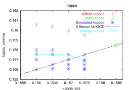
Figure 16: Our points of simulation in the hopping parameter plane of valence/sea quarks.

According to Ref. part_quen partial quenching of a particular quark species is achieved by introduction of scalar pseudoquark partners (of equal mass) that freeze those quark degress of freedom inside the determinant. In this context, one introduces a basis of states with $N_{q}$ quarks and $k$ additional pseudoquarks. In our situation, we have $N_{q}=5$ (three valence and two sea quarks) and $k=3$, if we allow for different masses of sea and valence quarks. The correlator has to make reference to these degrees of freedom, $i,j$. In Fourier space, it is modeled by the momentum space ansatz kilcup

$${\cal C}_{ij}=\frac{\delta_{ij}\epsilon_{i}}{p^{2}+m_{i}^{2}}-\frac{m_{0}^{2}}{(p^{2}+m_{i}^{2})(p^{2}+m_{j}^{2})F(p^{2})}\;\quad,i,j=1,2,\dots N_{q}+k\quad.$$ (80)

The quantity $\epsilon_{i}$ is equal to +1 (-1) for quark (pseudoquark = determinant eater) channels. The function $F(p^{2})$ can be viewed as to model the implicit multiloop contributions from sea quarks to the disconnected pole terms:

$$F(p^{2})=1+\sum_{\mbox{sea quarks }\sigma}\frac{m_{0}^{2}}{p^{2}+m_{\sigma}^{2}}\;.$$ (81)

$m_{i}$, $m_{j}$ and $m_{\sigma}$ denote neutral pseudoscalar nonsinglet meson masses, while $m_{0}$ refers to the effective singlet interaction that might depend on the quark species involved.

$F$ reads in the case of the SESAM simulation with degenerate dynamical $u$ and $d$ quarks

$$F(p^{2})=1+\frac{2m_{0}^{2}}{p^{2}+m_{\sigma}^{2}}\;.$$ (82)

Note that the model incorporates both the fully quenched limit, where $F(t)\equiv 1$, as well as the consistently $N_{f}=2$ unquenched situation, where $u$ and $d$ valence and dynamical quark masses coincide, such that $m_{1}=m_{2}=m_{\sigma}$: in this latter instance, the double pole term in the nonstrange sector is lifted and turned into a displaced single pole term, in accordance with the considerations presented in section 4.3.

For practical matters, a partially quenched lattice analysis of Eq. 80 is carried out in two steps as follows

1. The pseudoscalar meson masses, $m_{1},m_{2},m_{\sigma}$, are determined first by LQCD from connected pseudoscalar correlators with the appropriate valence quark settings (in the case of $m_{\sigma}$ and $m_{0,\sigma}$, sea and valence quark masses are identified),

2. the singlet correlator matrix contains a set of mass gap parameters, $m_{0,ij}$. They can be computed finally from a fit of the Fourier transform of the ansatz, Eq. (80), to the lattice data for ${\cal C}(t)$.

The latter fitting can be done time-slicewise, yielding fit parameters for ’local’ effective mass gaps which should exhibit mass plateau formation. It goes without saying that throughout all the numerical analysis steps one should use the dual filtering method with ’synthetic’ data in the sense of section 4.3.

5.3 Partially quenched results

In a comprehensive study ref:tsuk we analyzed some 800 independent SESAM configurations on $16^{3}\times 32$ lattices at $\beta=5.6$ ref:sesam , with four different sea quark masses. In Fig.16 we have plotted the set of hopping parameters of valence quarks in perspective with their critical values, for our different sea quark settings. The full QCD situation with 2 quark flavours in the sense of chapter 5.1 is indicated by the dotted line, $\kappa_{sea}=\kappa_{valence}$ and the thin line connects the hopping parameters for strange quarks.

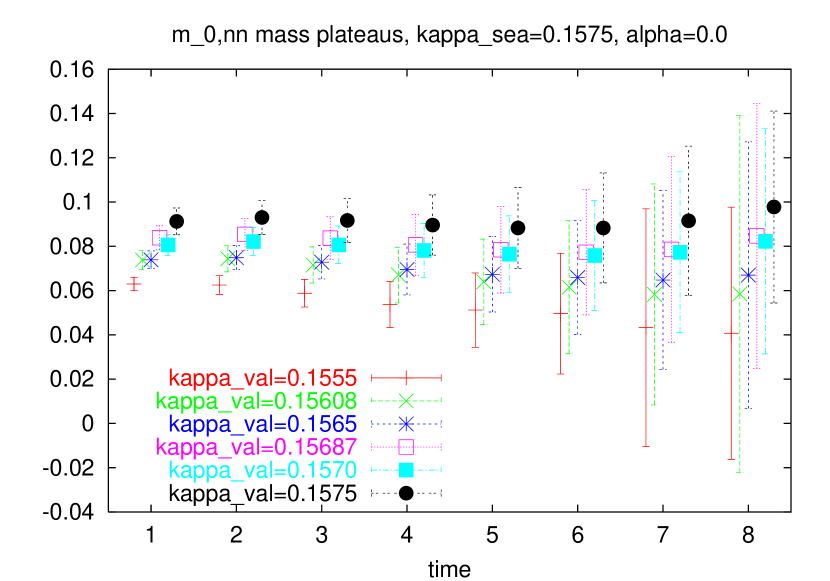
Figure 17: First evidence of plateau formation in a partially quenched setting, illustrated on the effective mass gap, $m_{0nn}(t)$, in the disconnected two loop correlator, $D_{nn}(t)$. The data refer to the lightest sea quark mass of SESAM, i.e. $\kappa_{sea}=.1575$, for various isosinglet valence quark masses.

We analyse the data according to Eq. 80. In doing so we proceed to study effective mass gaps as determined from the hairpin diagrams, $D_{ij}(t)$, by fitting, w.r.t. $m_{0ij}(t):=\mu$ at each value of $t$, the zero-momentum Fourier transforms of ansatz Eq. 80 to our data. In broken SU(3) with two active quark flavours, we introduce two isosinglet pseudoscalars, designated by the indices $n$ (for ‘light’, nonstrange) and $s$ (for strange). In this manner, we can study three types of hairpin diagrams, $D_{nn}$ , $D_{ns}$ , $D_{ss}$, with the strange quark mass determined on the lattice from the kaon mass (for $\kappa$ locations, see Fig.16). As a result, we find satisfying plateau formations in $m_{0ij}(t)$ as illustrated in Fig. 17. In fact, the numerical quality of our signals comfortably allows for the consecutive extrapolations (i) to light valence and then (ii) to light sea quark masses; the chiral sea quark extrapolation is exhibited in Fig. 18.

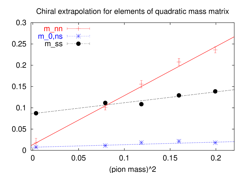
Figure 18: Extrapolations of the quadratic mass matrix elements of light ($n$) and strange ($s$) isosinglet valence quarks to QCD with chiral sea quarks (Eq. 85), at $\alpha=0$.

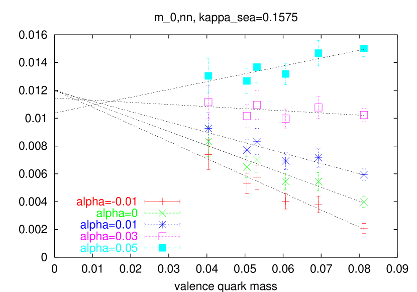
Figure 19: Minimizing the valence quark dependence of the mass gap by variation of $\alpha$.

From the consecutive chiral extrapolations, we obtain for the quadratic mass matrix in the quark-flavour basis

$${\cal M}:=\left(\begin{array}[]{cc}m^{2}_{nn}&m^{2}_{0,ns}\\ m^{2}_{0,sn}&m^{2}_{ss}\end{array}\right)\;,$$ (85)

where $m^{2}_{nn}:=M^{2}_{nn}+m^{2}_{0nn}$. With the $\rho$-meson mass scale sesam we find

$${\cal M}=\left(\begin{array}[]{cc}(306\pm 91)^{2}&\sqrt{2}(201\pm 34)^{2}\\ \sqrt{2}(201\pm 34)^{2}&(680\pm 15)^{2}\end{array}\right)\mbox{MeV}^{2}\;.$$ (88)

Diagonalization of $\cal M$ renders

$$M_{\eta}=292\pm 31\;\mbox{MeV},\quad M_{\eta^{\prime}}=686\pm 31\;\mbox{MeV}.$$ (89)

These numbers from $N_{f}=2$ look promising: the individual mass values – while being low w.r.t. the real three flavour world – yield a mass splitting that compares very well to phenomenology.

5.4 Data in accord to $\chi$PT?

So far we have neglected that the partially quenched scenario has been devised in the framework of chiral perturbation theory ($\chi$PT) where we expect to deal with a limited number of effective couplings. In fact, Bernard and Golterman part_quen showed that the effective chiral symmetry violation (due to the chiral anomaly) is most simply described by the following contribution to the chiral Lagrangian:

$${\cal L}_{0}=+\frac{N_{f}}{2}\Big{[}{\mu^{2}}(\eta^{\prime})^{2}+{\alpha}(\partial_{\mu}\eta^{\prime})^{2}\Big{]}\;,$$ (90)

i.e. in terms of just two constants, $\mu$ (mass gap in the chiral limit) and $\alpha$ (interaction parameter) only! If the tree approximation of $\chi$ PT to their partially quenching scenario holds, the simulation data should be fitted in terms of these two constants, irrespective of the (supposedly light!!) valence quark masses chosen. We will now address the question whether this is indeed the case. To this end we have to first rewrite the correlators, Eq. 80, by including the parameter $\alpha$. Actually, the Lagrangian translates into two-point correlation functions (propagators) for the neutral pseudoscalar quark bilinears

$$\Phi_{ii}(x)=\bar{q}_{i}(x)\gamma_{5}q_{i}(x)\;,$$ (91)

where the index $i$ runs over the quark and pseudoquark d.o.f. part_quen .

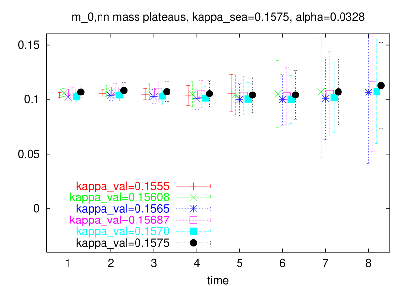
Figure 20: The analogue of Fig. 17: Universal plateau formation, at the lightest sea quark mass, when adjusting $\alpha$ to the value $0.0328$.

In momentum space the disconnected part of these ps-correlators again has a compact form ref:GP with the infamous double pole structure

$$D_{ij}(p)={\cal N}\frac{({\mu^{2}}+\alpha p^{2})(p^{2}+M_{d}^{2})}{(p^{2}+M_{ii}^{2})(p^{2}+M_{jj}^{2})(p^{2}+M_{\eta^{\prime}}^{2})}\;.$$ (92)

The prefactor, ${\cal N}=1/(1+N_{f}\alpha)$ and the singlet mass, $M^{2}_{\eta^{\prime}}=(M^{2}_{d}+N_{f}\mu^{2})/(1+N_{f}\alpha)$ are seen to carry explicit $\alpha$-dependencies. Rememeber that the octet masses ($M_{ii}$,$M_{jj}$, and $M_{d}$) from valence and sea quarks, respectively, are readily computed from connected diagrams on the lattice. Our present concern is the determination of the mass gap, $\mu$, and $\alpha$ from our lattice data.

We remark that the outcome of the analysis at this stage seems not to be in accord with the tree approximation to the Lagrangian, Eq. 91, as the latter predicts the mass plateaus to be independent of the valence quark mass, $m_{v}$, contrary to the apparant findings in Fig. 17. Therefore, we repeated the above mass plateau study on a set of nonvanishing $\alpha$-parameters, in an attempt to verify the compliance of our data with such independence: inspecting the plot of $m_{0nn}$ vs. $m_{v}$ (Fig. 19) it becomes obvious (i) that $m_{0nn}(m_{v})$ shows a simple, linear behaviour and (ii) that $\alpha$ can indeed be adjusted to produce a zero slope of $m_{0nn}(m_{v})$ !

In this way it is straightforward to find an optimal value, $\alpha_{opt}$, that eliminates (for a given sea quark mass) the $m_{v}$-dependence from $m_{0nn}$, resulting in a universal plateau level. This collapse of data into universal plateaus (of heights $\tilde{\mu}$) is exemplified in Fig. 20. The comparision with the situation encountered with $\alpha=0$ (Fig. 17) provides clear evidence for our sensitivity in determining $\alpha_{opt}$.

After chiral sea quark extrapolation we arrive at a first estimate of $\alpha$:

$$\alpha=0.028\pm 0.013\quad\mu=203\pm 34\mbox{MeV}\;.$$ (93)

Note that the numerical value for the mass gap at the chiral point is robust w.r.t. the two different approaches presented here. One might phrase it like this: the allowance for a nonvanishing $\alpha$ parameter is tantamount to the anticipation of the respective chiral valence quark limit in the mass gap!

6 Conclusion

The application of spectral techniques provides unprecedentedly high accuracy in the study of hairpin diagrams. Spectral methods thus provide access to detailed studies of the flavour singlet mesons. In this work, this has been demonstrated in two flavour QCD as well as in the $N_{f}=2$ partially quenched scenario, with standard Wilson fermions and in the regime of medium mass sea quarks (see Fig. 16. Since spectral methods are at their best in the truly chiral regime, this looks very promising in regard to future simulations of flavour singlet mesons with realistically light sea quarks, that we expect to come up within the overlap fermion formulation on the lattice.

References

-
(1)
S. Adler, Phys. Rev. 177, 2426 (1969),
J. Bell and R. Jackiw, Nuovo Cim. 60A, 47 (1969)
S. Adler and W.A. Bardeen, Phys. Rev. 182,1517 (1969). -
(2)
S. Okubo, Phys. Lett. 5, 165 (1963),
G. Zweig, CERN preprint TH412 (1964),
J. Iizuka, Progr. Theor. Phys. Suppl. 37-38 (1966) 21. - (3) R. Crewther, Phys. Lett. 70b, 349 (1977), Riv. Nuov. Cim. 2, 63 (1979), Acta. Phys. Austr. Suppl XIX, 47 (1978).
-
(4)
E. Witten, Nucl. Phys. B156, 269 (1979),
G. Veneziano Nucl. Phys. B159, 213 (1979) and Phys. Lett 95B, 90 (1980). - (5) L. Giusti, G.C. Rossi, M. Testa, and G. Veneziano, Nucl.Phys. B628, 234 (2002) and references quoted therein.
- (6) A. Frommer, V. Hannemann, B. Nöckel, Th. Lippert, and K. Schilling, Int. Journ. Mod. Phys 5,6 1073 (1994).
- (7) S. Duane, A.D. Kennedy, B.J. Pendleton, and D. Roweth, Phys. Lett. B195 216 (1987).
- (8) N. Eicker N. Eicker, P. Lacock, K. Schilling, A. Spitz, U. Glässner, S. Güsken, H. Hoeber, Th. Lippert, T. Struckmann, P. Ueberholz, J. Viehoff, and G. Ritzenhöfer (SESAM Coll.), Phys. Rev. D59, 14509 (1999).
- (9) S. Fischer, A. Frommer, U. Glässner, Th. Lippert, G. Ritzenhöfer, and K. Schilling, Comp. Phys. Comm. 98, 20 (1996).
- (10) H. Leutwyler, Nucl. Phys. Proc. Suppl. 64 223 (1998).
- (11) Th. Feldmann, P. Kroll, and B. Stech, Phys. Rev. D58 114006 (1998).
- (12) Th. Feldmann and P. Kroll, Eur. Phys.J C5 327 (1998), Th. Feldmann, P. Kroll, and B. Stech, Phys. Lett. B449 339 (1999).
- (13) P. Kroll and Th. Feldmann, Phys. Scripta T99 13 (2002).
- (14) M. Bochicchio, G. Martinelli, G. Rossi, and M. Testa, Nucl. Phys. B262 275 (1985).
- (15) L. Venkataraman and G. Kilcup, hep-lat79711006.
- (16) UKQCD C. McNeile et al (UKQCD Collaboration) Phys. Lett. B491 123 (2000), Erratum ibid. B551 391 (2003).
- (17) C. McNeile, C. Michael, and K.J. Sharkey,Phys.Rev. D65, 014508 (2002).
- (18) C. Michael, Phys.Scripta T99,7 (2002).
- (19) M. Lüscher and U. Wolff, Nucl. Phys. B339 222 (1990).
- (20) V.I Lesk, S. Aoki, R. Burkhalter, M. Fukugita, K.-I. Ishikawa, N. Ishizuka, Y. Iwasaki, K. Kanaya, Y. Kuramashi, M. Okawa, Y. Taniguchi, A. Ukawa, T. Umeda, and T. Yoshie, (CP-PACS Collaboration) Phys. Rev. D67 074503 (2003).
- (21) QCDSF M. Göckeler et al. (QCDSF collaboration) Phys. Lett. B545 112 (2002.
- (22) see e.g. W. Wilcox, Talk given at Interdisciplinary Workshop on Numerical Challenges in Lattice QCD, Wuppertal, Germany, 22-24 Aug 1999. Published in Wuppertal 1999, Numerical challenges in lattice quantum chromodynamics, hep-lat/9911013.
- (23) T. Struckmann, K. Schilling, G. Bali, N. Eicker, S. Güsken, T. Lippert, H. Neff, B. Orth, W. Schroers, J. Viehoff, and P. Ueberholz (SESAM and TL Coll.), Phys.Rev. D63 074503 (2001).
- (24) H. Neff, N. Eicker, Th. Lippert, J.W. Negele, and K. Schilling, Phys. Rev. 64 114509 (2001).
- (25) Y. Kuramashi, M. Fukugita, H. Mino, M. Okawa, and A. Ukawa, Phys. Rev. Lett. 72 3448 (1994).
- (26) C. Michael and J. Peisa, Phys. Rev. D58 034506 (1998).
- (27) H. Neff, Nucl. Phys. B106 (Proc.Suppl.) 1055 (2002), hep-lat/0110076.
- (28) H. Neff, T. Lippert, J.W. Negele, and K. Schilling, Nucl. Phys. B119 (Proc.Suppl.) 251 (2003), hep-lat/0209117.
- (29) H. Neff, Th. Lippert, J. Negele, and K. Schilling, contribution LATTICE2003.
- (30) C.W. Bernard and M. F.L. Golterman, Phys. Rev. D49 486 (1994).
- (31) N. Eicker et al (SESAM coll.) Phys. Letts. B407 (1997) 219.
- (32) M. Golterman et al, JHEP 0008 (2000) 023.
- (33) H. Neff et al, in preparation.