Connecting Lattice QCD with Chiral Perturbation Theory at Strong Coupling

Abstract

We study the difficulties associated with detecting chiral singularities predicted by chiral perturbation theory (ChPT) in lattice QCD. We focus on the physics of the remnant $O(2)$ chiral symmetry of staggered fermions in the strong coupling limit using the recently discovered directed path algorithm. Since it is easier to look for power-like singularities as compared to logarithmic ones, our calculations are performed at a fixed finite temperature in the chirally broken phase. We show that the behavior of the chiral condensate, the pion mass and the pion decay constant, for small masses, are all consistent with the predictions of ChPT. However, the values of the quark masses that we need to demonstrate this are much smaller than those being used in dynamical QCD simulations. We also need to use higher order terms in the chiral expansion to fit our data.

I INTRODUCTION

With the advent of fast computers it is now possible to calculate many hadronic quantities from first principles using lattice QCD. However, today these calculations contain systematic errors due to finite lattice spacings, finite volumes and quenching. Although in principle all these errors can be controlled, the only clean way to reduce quenching errors is to perform unquenched calculations. Due to algorithmic difficulties today most unquenched calculations are performed using large quark masses and the results are then extrapolated to realistic values using (quenched and partially quenched) ChPT. Unfortunately, recent attempts to connect lattice QCD with the usual one-loop ChPT predictions have failed to give clear answers JLQCD ; Dur02 ; Mon03 ; Ber02 . It is now believed that lattice artifacts should be taken into consideration in ChPT Lee99 ; Aub03 ; Rup02 ; Aok03 . It has been suggested in Aub03.a ; Far03 the lattice data is described better by the resulting more elaborate fitting functions. There are also other interesting attempts to extract useful information using finite size effects in ChPT Bie03 .

Given the difficulties associated with understanding chiral singularities in a realistic calculation of QCD, in this paper we explore the subject in strong coupling lattice QCD with staggered fermions. We use a very efficient algorithm discovered recently to solve this model in the chiral limit Ada03 . Although the strong coupling limit suffers from severe lattice artifacts, when the quarks are massless lattice QCD with staggered fermions has an exact $O(2)$ chiral symmetry which is broken spontaneously. Thus, our model contains some of the remnant physics of chiral singularities expected in QCD. In particular, there are light pions and it would be useful to understand the range of quark masses where the singularities predicted by conventional ChPT can be seen.

Instead of focusing on chiral singularities that are logarithmic, in this work we focus on power-like singularities that arise at finite temperatures. Recently, it was shown with high precision that our model undergoes a second order chiral phase transition at a critical temperature $T_{c}$. This transition belongs to the $O(2)$ universality class Cha03 . Thus, at a fixed temperature below $T_{c}$, within the the $O(2)$ scaling window, the long distance physics of our model is described by a three-dimensional $O(2)$ field theory in its broken phase. At this temperature there is a range of quark masses where the light pions are describable by the conventional continuum ChPT. The effective action can be written in terms of $\vec{S}$, an $O(2)$ vector field with the constraint $\vec{S}\cdot\vec{S}=1$. At the lowest order this is given by Has90

$$S_{\rm eff}=\int d^{3}x\Big{[}\ \frac{F^{2}}{2}\ \partial_{\mu}\vec{S}\cdot\partial_{\mu}\vec{S}+\Sigma\ \vec{h}\cdot\vec{S}\Big{]}$$ (1)

where $\vec{h}$ is the magnetic field and $|\vec{h}|$ is identified with the quark mass. The two low energy constants $F^{2}$ and $\Sigma$ that appear at this order are the pion decay constant and the chiral condensate respectively. We note that since we are discussing a three-dimensional effective theory, $F^{2}$ has the dimensions of inverse length. Thus, we can define a correlation length $\xi\equiv 1/F^{2}$. For massless quarks $\xi$ diverges as $(T_{c}-T)^{-\nu}$ at $T_{c}$. In order to connect our model with ChPT and avoid lattice artifacts we need to choose the temperature and quark masses such that $1<<\xi<<1/M_{\pi}$ (lengths are measured in lattice units) where $M_{\pi}$ is the pion mass. In this region we expect observables such as the chiral condensate, the pion mass and the pion decay constant satisfy the expansion

$$\langle O\rangle=z_{0}+z_{1}\sqrt{m}+z_{2}m+z_{3}m\sqrt{m}+...,$$ (2)

where the $\sqrt{m}$ behavior is the power-like singularity arising due to the infrared pion physics Wal75 . The main objective of this paper is to detect these singularities in the context of strong coupling lattice QCD with staggered fermions. Such power-like singularities have been observed in spin models Eng01 , but as far as we know have not been studied with precision in lattice QCD calculations.

II The Model and Observables

The partition function of the model we study in this article is given by

$$Z(T,m)=\int[dU][d\psi d\bar{\psi}]\ \exp\left(-S[U,\psi,\bar{\psi}]\right),$$ (3)

where $[dU]$ is the Haar measure over $U(3)$ matrices and $[d\psi d\bar{\psi}]$ specify Grassmann integration. At strong coupling, the Euclidean space action $S[U,\psi,\bar{\psi}]$ is given by

$$-\sum_{x,\mu}\frac{\eta_{x,\mu}}{2}\Big{[}\bar{\psi}_{x}U_{x,\mu}\psi_{x+\hat{\mu}}-\bar{\psi}_{x+\hat{\mu}}U^{\dagger}_{x,\mu}\psi_{x}\Big{]}-m\sum_{x}\bar{\psi}_{x}\psi_{x},$$ (4)

where $x$ refers to the lattice site on a periodic four-dimensional hyper-cubic lattice of size $L$ along the three spatial directions and size $L_{t}$ along the euclidean time direction. The index $\mu=1,2,3,4$ refers to the four space-time directions, $U_{x,\mu}\in U(3)$ is the usual links matrix representing the gauge fields, and $\psi_{x},\bar{\psi}_{x}$ are the three-component staggered quark fields. The gauge fields satisfy periodic boundary conditions while the quark fields satisfy either periodic or anti-periodic boundary conditions. The factors $\eta_{x,\mu}$ are the well-known staggered fermion phase factors. We choose them to be $\eta_{x,\mu}^{2}=1,\mu=1,2,3$ (spatial directions) and $\eta_{x,4}^{2}=T$ (temporal direction), where the real parameter $T$ acts like a temperature. By working on asymmetric lattices with $L_{t}<<L$ at fixed $L_{t}$ and varying $T$ continuously one can study finite temperature phase transitions in strong coupling QCD Boy92 . We use $U(3)$ gauge fields instead of $SU(3)$ in order to avoid inefficiencies in the algorithm due to the existence of baryonic loops. This distinction is not important for our study since the baryons are expected to have a mass close to the cutoff.

The partition function given in Eq. (3) can be rewritten in a monomer-dimer representation as discussed in detail in Ros84 ; Cha03 . Every configuration in the new representation is described by monomer variables $n_{x}=0,1,2,3$ associated to the sites, and dimer variables $b_{x,\mu}=0,1,2,3$ associated to the bonds connecting neighboring sites $x$ and $x+\hat{\mu}$, along with the constraint that at each site, $n_{x}+\sum_{\mu}[b_{x,\mu}+b_{x-\hat{\mu},\mu}]=3$.

In order to study chiral physics we focus on the following observables:

• The chiral condensate

  $$\langle\phi\rangle=\frac{1}{L^{3}}\frac{1}{Z}\frac{\partial}{\partial m}Z(T,m),$$ (5)

• the chiral susceptibility

  $$\chi=\frac{1}{L^{3}}\frac{1}{Z}\frac{\partial^{2}}{\partial m^{2}}Z(T,m),$$ (6)

• the helicity modulus

  $$Y=\frac{1}{L^{3}}\Bigg{\langle}\Big{\{}[\sum_{x}J_{x,1}]^{2}+[\sum_{x}J_{x,2}]^{2}+[\sum_{x}J_{x,3}]^{2}\Big{\}}\Bigg{\rangle},$$ (7)

  where $J_{x,\mu}=\sigma_{x}(b_{x,\mu}-N/8)$, with $\sigma_{x}=1$ on even sites and $\sigma_{x}=-1$ on odd sites and

• the pion mass, obtained using the exponential decay of the correlation function along one of the spatial directions $\mu=1,2,3$:

  $$\lim_{|x_{\mu}|\rightarrow\infty}\sum_{x_{\perp}}\langle\sigma_{x}n_{x}n_{0}\rangle=C\mathrm{e}^{-M_{\pi}|x_{\mu}|},$$ (8)

where $x_{\perp}$ refers to components of the coordinate $x$ perpendicular to the $\mu$ direction. When $m=0$ the current $J_{x,\mu}$ is the conserved current associated with the $O(2)$ chiral symmetry. As discussed in Has90 , one can define the pion decay constant at a quark mass $m$ to be $F_{m}^{2}\equiv\lim_{L\rightarrow\infty}Y$. For $m=0$ we then obtain $F=\lim_{m\rightarrow 0}F_{m}$, the pion decay constant introduced in Eq.(1). We can also define $\Sigma_{m}=\lim_{L\rightarrow\infty}\langle\phi\rangle$ the infinite volume chiral condensate. Again $\Sigma=\lim_{m\rightarrow 0}\Sigma_{m}$.

III Results

We have done extensive computations at $L_{t}=4$. It has been shown with high precision in Cha03 that this model undergoes a chiral phase transition which belongs to the three-dimensional $O(2)$ universality class at a critical temperature $T_{c}=7.47739(3)$. Figure 1 shows the plot of $F^{2}$ as a function of $T$. Based on universality we expect $\xi^{-1}\equiv F^{2}=C(T_{c}-T)^{\nu}$ for $T<T_{c}$ with $\nu=0.67155(27)$ Cam01 . If we fit our results to this form in the range $7.05\leq T\leq 7.42$, with $T_{c}$ and $\nu$ fixed to the expected values, we find $C=0.2217(1)$ with $\chi^{2}/$DOF$=1.03$. Including $T=7.0$ in the fit makes the $\chi^{2}$/DOF jump to $2.0$.

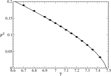
Figure 1: Plot of $F^{2}$ vs. $T$. The solid line represents the function $0.2217(7.47739-T)^{0.67155}$.

At a temperature very close to $T_{c}$, we expect $\xi$ to be extremely large and it would be difficult to satisfy $1/M_{\pi}>>\xi$ with our limited computing resources. On the other hand in order to avoid lattice artifacts it is important not to have $\xi\sim 1$. Using the above analysis we estimate that $T=7.0$ is at the edge of the $O(2)$ scaling window and hence we choose to fix $T$ at this value and study the long distance physics near the chiral limit. We vary the spatial lattice size from $L=8$ to $L=96$ for a variety of masses $0\leq m\leq 0.025$. At $m=0$ we also have data at $L=120,144$. Below we discuss our main results.

III.1 The Pion Decay Constant

Our results show that for $L\geq 32$ the finite size effects on $Y$ are smaller than the statistical errors. Hence it is relatively easy to compute $F_{m}^{2}$ by extrapolating results for $Y$ at different volumes. In Table 1 we give the results for some values of the quark mass.

$m$	$F_{m}$	$m$	$F_{m}$
0.00000	0.3675(1)	0.0050	0.4063(1)
0.00025	0.3703(1)	0.0075	0.4188(1)
0.00050	0.37300(15)	0.0100	0.42890(15)
0.00100	0.37804(15)	0.0200	0.4583(2)
0.0025	0.3903(2)	0.0250	0.4693(2)

Table 1: $F_{m}$ as a function of $m$.

The first four terms in the chiral expansion of $F_{m}$ in three-dimensional $O(N)$ ChPT are given by Has90

$$F_{m}=F[1+a_{1}\sqrt{m}+a_{2}m+a_{3}m\sqrt{m}],$$ (9)

where $a_{1}\propto(N-2)$. Since in our case $N=2$ we expect $a_{1}=0$.

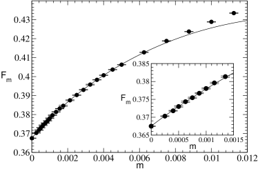
Figure 2: Plot of $F_{m}$ vs. $m$. The solid line represents the function $F_{m}=0.36747[1+34.2m-185m\sqrt{m}]$.

In order to check if our results fit the predictions of ChPT we fit our data to Eq.(9) in the range $0\leq m\leq 0.00625$. We find $F=0.3674(1)$, $a_{1}=0.01(2)$, $a_{2}=34.0(7)$ and $a_{3}=-182(6)$ with $\chi^{2}$/DOF$=1.2$. Our data and the fit are shown in Fig. 2. The prediction of ChPT that $a_{1}=0$ is in excellent agreement with our results. Fixing $a_{1}=0$ in the fit yields $F=0.36747(6)$, $a_{2}=34.3(3)$ and $a_{3}=-185(3)$, while the $\chi^{2}$/DOF remains essentially unchanged. Interestingly if we fit the data in the range $0\leq m\leq 0.00135$ with $a_{1}=a_{3}=0$ fixed, we find that $F=0.36764(7)$ and $a_{2}=28.3(3)$ with $\chi^{2}$/DOF$=0.9$. This shows that there are systematic errors in evaluating the fitting parameters due to contamination from higher order terms. In the inset of Fig. 2 we focus on the extremely small mass region and show that $a_{1}=0$ is even clear to the eye. This is one of the main results of our paper. We suggest that $a_{1}=0$ is a useful signature of the $O(2)$ universality and could be used in future studies of lattice QCD with staggered fermions.

III.2 The Chiral Condensate

Chiral perturbation theory predicts that the first four terms in the chiral expansion of $\Sigma_{m}$ are given by

$$\Sigma_{m}=\Sigma[1+b_{1}\sqrt{m}+b_{2}m+b_{3}m\sqrt{m}].$$ (10)

As shown in Has90 , $b_{1}\propto(N-1)$, implying that $b_{1}\neq 0$ in our case. In order to test how well Eq. (10) describes our model, we compute $\Sigma_{m}$ at small masses.

At $m=0$ we compute $\Sigma$ by using the finite size scaling formula for $\chi$ given by Has90

$$\chi=\frac{1}{N}\Sigma^{2}L^{3}\Big{[}1+0.226(N-1)\frac{1}{F^{2}L}+\frac{\alpha}{L^{2}}+...\Big{]},$$ (11)

where $\alpha$ depends on the higher order low energy constants of the chiral Lagrangian. When $F$ is fixed to $0.3675$ obtained earlier, our results for $16\leq L\leq 144$ fit very well to this formula. We find $\Sigma=2.2648(10)$, $\alpha=4.6(3)$ with $\chi^{2}$/DOF$=0.87$.

$m$	$\Sigma_{m}$	$m$	$\Sigma_{m}$
0.00000	2.2648(10)	0.0050	2.6340(08)
0.00025	2.2340(10)	0.0075	2.7278(15)
0.00050	2.3560(10)	0.0100	2.8025(15)
0.00100	2.4040(05)	0.0200	3.0199(11)
0.0025	2.5103(08)	0.0250	3.0986(08)

Table 2: Values of $\Sigma_{m}$ at selected values of $m$.

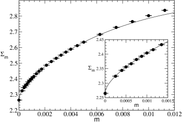
Figure 3: Plot of $\Sigma_{m}$ vs. $m$. The solid line represents the function $\Sigma_{m}=2.2642[1+1.36\sqrt{m}+23m-135m\sqrt{m}]$.

For $m\neq 0$ one can measure $\Sigma_{m}$ by extrapolating the results for $\langle\phi\rangle$ at different volumes. However, due to critical slowing down it is difficult to measure the condensate accurately at a fixed small mass on large volumes. With our computing resources we find that this procedure gives reliable answers for $\Sigma_{m}$ only up to $m\sim 0.001$. On the other hand when $m\neq 0$, in the large volume limit we expect $\chi\sim\Sigma_{m}^{2}L^{3}$ up to an additive constant plus exponentially small corrections. We find that the signal for $\Sigma_{m}$ extracted from fitting the data to this form is much cleaner at small masses than the signal obtained from the direct measurement. Further, the values of $\Sigma_{m}$ obtained using this procedure agree well with the direct measurement at larger quark masses. In table 2 we give the values of $\Sigma_{m}$ obtained for selected values of the quark masses. Fitting our results to Eq.(10) in the region $0\leq m\leq 0.00625$ gives $\Sigma=2.2642(10)$, $b_{1}=1.36(4)$, $b_{2}=23(1)$, $b_{3}=-135(10)$ with a $\chi^{2}$/DOF$=1.1$. Our results are shown in Fig 3. We note that we cannot find a mass range within our results in which we can find a good fit when we fix $b_{2}=b_{3}=0$. However, in the range $0\leq m\leq 0.00175$ we can set $b_{3}=0$ to obtain $\Sigma=2.2643(10)$, $b_{1}=1.44(3)$ and $b_{2}=15.2(7)$ with a $\chi^{2}$/DOF$=1$. Note that $b_{2}$ changes by about 30% when this different fitting procedure is used, while $b_{1}$ is more stable.

$m$	$\Sigma_{m}$	$m$	$\Sigma_{m}$
0.00000	0.000	0.0050	0.2812(8)
0.00025	0.0650(3)	0.0075	0.3399(5)
0.00050	0.0920(4)	0.0100	0.3871(4)
0.00100	0.1295(4)	0.0200	0.5285(10)
0.0025	0.2022(3)	0.0250	0.5837(8)

Table 3: Values of $M_{\pi}$ at selected values of $m$.

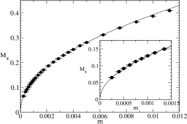
Figure 4: Plot of $M_{\pi}$ vs. $m$. The solid line represents the function $M_{\pi}=4.095\sqrt{m}[1+0.68\sqrt{m}-25.8m+149m\sqrt{m}]$.

III.3 The Pion Mass

The first four terms in the chiral behavior of the pion mass are predicted to be of the form

$$M_{\pi}=\sqrt{\frac{\Sigma}{F^{2}}}\sqrt{m}\Big{[}1+c_{1}\sqrt{m}+c_{2}m+c_{3}m\sqrt{m}\Big{]}.$$ (12)

Further, the chiral Ward identities imply that $c_{1}=b_{1}/2-a_{1}$. Our estimates for the pion masses for a selected range of $m$ are shown in Table 3. Fitting our data to Eq.(12) after fixing $\Sigma=2.2648$ and $F=0.3675$ obtained above, we find $c_{1}=0.55(16)$, $c_{2}=-21(6)$ and $c_{3}=110(50)$ with $\chi^{2}/$DOF$=0.5$. We see that our data is consistent with the relation $c_{1}=b_{1}/2-a_{1}$ although the error in $c_{1}$ is large. Fixing $c_{1}=b_{1}/2=0.68$ obtained from fitting the chiral condensate, yields $c_{2}=-25.8(8)$ and $c_{3}=149(14)$ without changing the quality of the fit. This latter fit along with our results for $M_{\pi}$ are shown in Fig. 4.

IV DISCUSSION

It is expected that the natural expansion parameter for ChPT in three dimensions is $x\equiv M_{\pi}/(4\pi F^{2})$. Let us find the values of $x$ where the chiral expansion up to a certain power of $x$ is sufficient to describe the data reasonably. Of course this question is model-dependent, since some models may have larger contributions at higher orders compared to others. Here we ask this question in the context of the model studied in this paper.

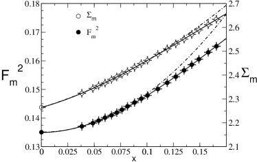
Figure 5: Plot of $F^{2}_{m}$ and $\Sigma_{m}$ vs. $x\equiv M_{\pi}/(4\pi F^{2})$. The solid lines and dot-dashed lines are fits to two different orders of chiral expansion discussed in the text.

In order to understand the dependence of $F^{2}_{m}$ and $\Sigma_{m}$ on $x$ we plot in Fig. 5 these two observables as functions of $x$. The solid lines are the best fits to the form $z_{0}+z_{1}x+z_{2}x^{2}+z_{3}x^{3}$, while the dot-dashed lines are the best fits to a smaller range in $x$ with $z_{3}$ set to $0$. As the graph indicates the error in $\Sigma_{m}$ due to the absence of the $z_{3}$ term is different from the error in $F_{m}^{2}$ at a given value of $x$. In order to determine $F_{m}^{2}$ within say $5\%$ we need the $z_{3}$ term even at $x\sim 0.15$. This shows that our model contains important higher order terms. An interesting question which we cannot answer at this point is whether this property is generic or not. In any case we have shown that the connection of lattice QCD data to ChPT is indeed possible as long as one does not assume that higher order terms are negligible. For the lowest order terms to dominate it may be necessary to go to much smaller quark mases than has been possible until now. In fact it is much easier to connect our results with ChPT at $m=0$, which is called the $\epsilon$-regime of ChPT Bie03 . Thus, finding an algorithm to work directly at $m=0$ is a useful goal to strive for in the future. Finally we hope that our results will motivate further work to uncover the power-law chiral singularities at finite temperatures in Lattice QCD at weaker couplings. This should be easier than looking for logarithmic singularities at zero temperature.

References

- (1) S. Hashimoto et. al., Nucl. Phys. (Proc.Suppl.) 119, 332 (2003).
- (2) S. Dürr, arXiv: hep-lat/0209319.
- (3) I. Montvay, arXiv: hep-lat/0301013.
- (4) C. Bernard et. al., Nucl. Phys. B. (Proc. Suppl.) 119, 170 (2003).
- (5) W. Lee and S. Sharpe, Phys. Rev. D60, 114503 (1999).
- (6) C. Aubin and C. Bernard, arXiv:hep-lat/0308036.
- (7) G. Rupak and N. Shoresh, Phys. Rev. D66, 054503 (2002).
- (8) S. Aoki, Phys. Rev. D68, 054508 (2003).
- (9) C. Aubin et. al., arXiv:hep-lat/0309088.
- (10) F. Farchioni, I. Montvay, E. Scholz and L. Scorzato, Eur. Phys. J. C31, 227 (2003).
- (11) W. Bietenholz, T. Chiarappa, K. Jansen, K.I. Nagai and S. Shcheredin, arXiv:hep-lat/0311012.
- (12) D. H. Adams and S. Chandrasekharan, Nucl. Phys. B662, 220 (2003).
- (13) S. Chandrasekharan and F.J.Jiang, Phys. Rev. D68, 091501(R) (2003).
- (14) P. Hasenfratz and H. Leutwyler, Nucl. Phys. B343, 241 (1990).
- (15) D.J. Wallace and R.K.P.Zia, Phys. Rev. B12, 5340 (1975).
- (16) J. Engels, S. Holtmann, T. Mendez and T. Schulze, Phys. Lett. B514, 299 (2001).
- (17) G. Boyd, J. Fingberg, F. Karsch, L. Karkkainen and B. Petersson Nucl. Phys. B376, 199 (1992).
- (18) P. Rossi and U. Wolff, Nucl. Phys. B248, 105 (1984).
- (19) M. Campostrini, M. Hasenbusch, A. Pelissetto, P. Rossi and E. Vicari, Phys. Rev. B63, 214503 (2001).