The photon propagator in compact QED₂₊₁:
the effect of wrapping Dirac strings

Abstract

We discuss the influence of closed Dirac strings on the photon propagator in the Landau gauge emerging from a study of the compact $U(1)$ gauge model in $2+1$ dimensions. This gauge also minimizes the total length of the Dirac strings. Closed Dirac strings are stable against local gauge-fixing algorithms only due to the torus boundary conditions of the lattice. We demonstrate that these left-over Dirac strings are responsible for the previously observed unphysical behavior of the propagator of space-like photons ($D_{T}$) in the deconfinement (high temperature) phase. We show how one can monitor the number $N_{3}$ of thermal Dirac strings which allows to separate the propagator measurements into $N_{3}$ sectors. The propagator in $N_{3}\neq 0$ sectors is characterized by a non–zero mass and an anomalous dimension similarly to the confinement phase. Both mass squared and anomalous dimension are found to be proportional to $N_{3}$. Consequently, in the $N_{3}=0$ sector the unphysical behavior of the $D_{T}$ photon propagator is cured and the deviation from the free massless propagator disappears.

I Introduction

The interest in the three-dimensional compact electrodynamics (cQED₃) has two roots: (i) this model shares similar features with QCD such as confinement Polyakov and chiral symmetry breaking ChSB and (ii) cQED₃ has applications to condensed matter systems such as Josephson junction arrays Josephson and high-$T_{c}$ superconductors HighTc . All non-perturbative features of cQED₃ arise thanks to the compactness of the gauge field, which, in turn, leads to the appearance of monopoles. The monopole plasma at low temperature phase gives rise to the confinement of electric charges Polyakov whereas at high temperature the confinement disappears due to binding of monopoles and antimonopoles into dipoles AgasianZarembo ; Chernodub:2001ws .

The confinement property manifests itself also in the gauge boson propagator in the Landau gauge Chernodub:2001mg . The effect is twofold: first, an ”anomalous dimension” $\alpha$ appears which modifies the momentum dependence of the propagator, and second, a mass $m$ is generated which can be well understood in terms of Polyakov’s theory Polyakov . As it is shown in Ref. Chernodub:2001mg , all nontrivial effects reside exclusively in the singular fields of the monopoles. At the critical temperature – where the monopole plasma turns into the dipole plasma – both effects disappear.

The monopole binding is observed in the zero-temperature model, too, in the presence of matter fields. At sufficiently strong coupling between gauge and matter fields the monopole plasma also turns into a dipole plasma AnomalousMatter ; Chernodub:2002ym . At weak coupling the dynamical matter fields have some influence on the anomalous dimension of the gauge boson propagator AnomalousMatter ; Chernodub:2002en .

Once monopoles and antimonopoles have turned into pairs they cannot contribute to non-perturbative effects like anomalous dimension and mass generation. Therefore it is natural to expect that in the high temperature phase of cQED₃ the masses and anomalous dimensions characterizing the photon propagator have to vanish. However, the numerical results of Ref. Chernodub:2002gp seem to indicate the existence of a non-zero mass and anomalous dimension for the propagator of the spatial photons even in the high temperature (deconfinement) phase. It was suggested in Ref. Chernodub:2002gp that the spatial photons are affected by a severe Gribov copy problem which might lead to unphysical results in the Landau gauge.

The fact that the $U(1)$ gauge theory in four space-time dimensions has a gauge fixing problem related to the Dirac strings was discussed in Ref. Valya:DDS . It was pointed out there that those gauge copies which possess so-called double Dirac sheets (DDS) give rise to a wrong behavior of the gauge boson propagator.

The DDS is a classical solution in the $U(1)$ gauge model Valya:classical that can be considered as a world surface of a tightly bound pair of oppositely ”charged” Dirac strings. The configuration containing a DDS is a Gribov copy of another configuration with zero number of double sheets. The DDS’s are closed by wrapping around the lattice torus and are not associated with any monopoles. It was shown in Ref. Valya:DDS that the practical removal of the DDS’s is a quite delicate problem.

In the present paper we study the gauge boson propagator in high-temperature cQED₃. We focus on gauge configurations containing Dirac strings looping along the shortest compactified (i.e. temperature) direction. Below we shall call these loops ”thermal Dirac loops” (TDL). We will show that configurations without such closed Dirac loops provide physically sane results (vanishing anomalous dimension and mass: $\alpha=0$, $m=0$) for the propagator in the Landau gauge whereas the presence of even a single closed Dirac loop leads to a non-vanishing $\alpha$c and $m$. We do not search for the double Dirac loops of opposite orientation (a three–dimensional analog of the double Dirac sheet discussed in Ref. Valya:DDS ). In our approach those double Dirac loops would be treated as two Dirac strings.

In Section II we recall the lattice model and remind the tensorial structure of the photon propagator at $T\neq 0$. In Section III we present the numerical results establishing the relation between parameters of the photon propagator and closed Dirac loops. Our conclusions are formulated in the last Section.

II The model and its photon propagator at finite $T$

In this Section we briefly describe the model, the structure of the propagator and the algorithms which were used in our work. All these technical details are the same as described in our earlier paper Chernodub:2002gp . An interested reader may consult that paper for a more detailed description.

We use the standard Wilson single-plaquette action of cQED₃,

$$S[\theta_{l}]=\beta\sum\limits_{p}\big{(}1-\cos\theta_{p}\big{)}\,,$$ (1)

where $\theta_{p}$ is the $U(1)$ field strength tensor represented by the plaquette curl of the compact link field $\theta_{l}$. The lattice coupling constant $\beta$ is related to the lattice spacing $a$ and the continuum coupling constant $g_{3}$ – which has dimension ${\mathrm{mass}}^{1/2}$ – of the $3D$ theory as follows:

$$\beta=1/(a\,g^{2}_{3})\;.$$ (2)

The lattice corresponding to finite temperature is asymmetric, $L^{2}_{s}\times L_{t}$, $L_{t}\ll L_{s}$. In the limit $L_{s}\to\infty$, the temporal extension of the lattice is related to the physical temperature, $L_{t}=1/(Ta)$. Using (2) the temperature can be expressed in units of $g_{3}^{2}$ in the following way:

$$\frac{T}{g^{2}_{3}}=\frac{\beta}{L_{t}}\,.$$ (3)

Thus the temperature $T$ is proportional to the lattice coupling $\beta$: the low-temperature (confinement) phase is realized at small values of $\beta$, the high-temperature (deconfinement) phase corresponds to large $\beta$.

All our simulations are performed on a $32^{2}\times 8$ lattice. For this lattice the phase transition happens at Chernodub:2001ws $\beta_{c}=2.30(2)$. In the confinement phase the density of the monopoles is relatively high. The gauge dependent Dirac string bits through Dirac plaquettes defined below (and needed to construct the gauge independent monopoles) form either connected clusters of open Dirac strings with monopoles and antimonopoles at their ends or clusters of closed strings. Therefore, for a high monopole density the number of Dirac strings is large, too.

In this paper we are interested in the quantitative effects of the temporal Dirac strings. Therefore we would prefer to work at low monopole densities in order to be able to easily separate closed and open Dirac strings unambiguously. We are going to present a quantitative demonstration that thermal Dirac loops create an unphysical behavior of the transverse photon propagator due to our attempt to fix the configuration to Landau gauge. Thus, we have chosen to illustrate this by a simulation at $\beta=2.6$ which is located already deep in the deconfinement phase. At this value of $\beta$ the density of the monopoles is quite low, $\rho_{\mathrm{mon}}=1.5(2)\cdot 10^{-4}$, compared to the confinement phase (where, for example, $\rho_{\mathrm{mon}}=0.1950(1)$ at $\beta=1.0$). We have mentioned already that the construction of the Dirac string is gauge dependent. An ideal Landau gauge fixing makes the open strings between the remaining monopoles and antimonopoles (in the form of dipoles) straightened, whereas the closed ones, if not “wrapping”, will collapse.

The final discussion of the photon propagator will be given in lattice momentum space. With the vector potential $A_{{\vec{x}},\mu}$ defined in a specified gauge, the propagator is written in terms of the Fourier transformed gauge potential,

$$\tilde{A}_{{\vec{k}},\mu}=\frac{1}{\sqrt{L_{1}~{}L_{2}~{}L_{3}}}\sum\limits_{{\vec{n}}}\exp\Bigl{(}2\pi i~{}\sum_{\nu=1}^{3}\frac{k_{\nu}(~{}n_{\nu}+\frac{1}{2}\delta_{\nu\mu}~{})}{L_{\nu}}\Bigr{)}~{}A_{{\vec{n}}+\frac{1}{2}{\vec{\mu}},\mu}\;,$$ (4)

which is a sum over a certain discrete set of points ${\vec{x}}={\vec{n}}+\frac{1}{2}{\vec{\mu}}$ forming the support of $A_{{\vec{x}},\mu}$ on the lattice. These are the midpoints of the links in $\mu$ direction. Here ${\vec{n}}$ denotes the lattice sites (nodes) with integer Cartesian coordinates. The propagator is the gauge-fixed ensemble average of the following bilinear in $\tilde{A}$,

$$D_{\mu\nu}({\vec{p}})=\langle\tilde{A}_{{\vec{k}},\mu}\tilde{A}_{-{\vec{k}},\nu}\rangle\;.$$ (5)

We use the sine-definition of the gauge potential:

$$A_{{\vec{n}}+\frac{1}{2}{\vec{\mu}},\mu}=\sin\left(\theta_{{\vec{n}},\mu}\right)/(g_{3}~{}a)=\left(U_{{\vec{n}},\mu}-U^{*}_{{\vec{n}},\mu}\right)/(2~{}i~{}g_{3}~{}a)\,.$$ (6)

The lattice momenta ${\vec{p}}$ on the left hand side of (5) are related to the integer valued Fourier momenta ${\vec{k}}$ as follows:

$$p_{\mu}(k_{\mu})=\frac{2}{a}\sin\frac{\pi k_{\mu}}{L_{\mu}}\,,\quad k_{\mu}=0,\pm 1,...,\pm\frac{L_{\mu}}{2}\;.$$ (7)

In the finite temperature case, the propagator can be parameterized by three scalar functions (formfactors),

$$D_{\mu\nu}({\vec{p}})=P^{T}_{\mu\nu}({\vec{p}})D_{T}(|{\mathbf{p}}|,p_{3})+P^{L}_{\mu\nu}({\vec{p}})D_{L}(|{\mathbf{p}}|,p_{3})+\frac{p_{\mu}p_{\nu}}{p^{2}}\frac{F(|{\mathbf{p}}|,p_{3})}{p^{2}}\,,$$ (8)

where we have identified the temperature direction with the $\mu=3$ axis, and have introduced the notations ${\mathbf{p}}^{2}=p_{1}^{2}+p_{2}^{2}$ and $|{\mathbf{p}}|=\sqrt{{\mathbf{p}}^{2}}$. If the Landau gauge is exactly fulfilled, one would expect that $F(p^{2})\equiv 0$. In our simulations presented below this function is indeed very close to zero.

Eq. (8) contains also two projection operators, namely, the transverse (with respect to the temperature direction) projection operator $P^{T}$ and the two-dimensional longitudinal projection operator $P^{L}$, respectively (with $i,j=1,2$),

$$P^{T}_{ij}({\vec{p}}) = \delta_{ij}-\frac{p_{i}p_{j}}{{\mathbf{p}}^{2}}\,,\quad P^{T}_{33}({\vec{p}})=P^{T}_{3i}({\vec{p}})=P^{T}_{i3}({\vec{p}})=0\,,$$ (9)

$$P^{L}_{\mu\nu}({\vec{p}}) = P_{\mu\nu}({\vec{p}})-P^{T}_{\mu\nu}({\vec{p}})\,,\quad P_{\mu\nu}({\vec{p}})=\delta_{\mu\nu}-\frac{p_{\mu}p_{\nu}}{p^{2}}\,.$$ (10)

In the static limit, $p_{3}=0$, the scalar function $D_{L}$ is equivalent to the correlator of temporal photons $D_{L}(|{\mathbf{p}}|,p_{3}=0)\equiv D_{33}(|{\mathbf{p}}|,p_{3}=0)$. The properties of this type of propagator have been discussed in Ref. Chernodub:2001mg . Analogously, the scalar function $D_{T}$ describes the behavior of the spatial photons. The behavior of this formfactor $D_{T}$ is of special interest in the present paper.

In order to analyze the effect of the Dirac strings on the propagator in general we separate singular (monopole) and regular (photon) contributions to the lattice gauge field on the level of the link angles $\theta_{l}$ following Refs. PhMon ; Chernodub:2001mg ; Chernodub:2002gp ; Chernodub:2002en ,

$$\theta=\theta^{\mathrm{phot}}+\theta^{\mathrm{mono}}\,,\quad\theta^{\mathrm{mono}}=2\pi\Delta^{-1}\delta p[j]\,,$$ (11)

where the dual zero-form $\mbox{}^{\ast}j$ represents the monopoles on the dual lattice sites ($i.e.$ the monopoles are defined on the cubes of the original lattice), $\Delta^{-1}$ is the inverse lattice Laplacian. The one-form on the dual lattice $p[j]$ defines the Dirac strings that connect monopoles and antimonopoles because of the condition $\delta\mbox{}^{\ast}p[j]=\mbox{}^{\ast}j$.

The photon part $\theta^{\mathrm{phot}}$ is free of singularities whereas the monopole part $\theta^{\mathrm{mono}}$ contains the information about the monopole and Dirac string singularities:

$$\frac{1}{2\pi}\mathrm{d}{[\mathrm{d}\theta^{\mathrm{phot}}]}_{2\pi}=0\,,\quad\frac{1}{2\pi}\mathrm{d}{[\mathrm{d}\theta^{\mathrm{mono}}]}_{2\pi}=j\,.$$ (12)

Here the DeGrand-Toussaint definition of the monopole DGT was used. Thus, besides the total propagator (5) below we will also study the singular contribution to the propagator, $D^{\mathrm{mono}}({\vec{p}})=\langle\tilde{A}^{\mathrm{mono}}_{{\vec{k}},\mu}\tilde{A}^{\mathrm{mono}}_{-{\vec{k}},\nu}\rangle$, and regular contribution $D^{phot}_{\mu\nu}({\vec{p}})=\langle\tilde{A}^{phot}_{{\vec{k}},\mu}\tilde{A}^{phot}_{-{\vec{k}},\nu}\rangle$. The total contains also the mixed contribution $D^{mixed}_{\mu\nu}({\vec{p}})=\langle\tilde{A}^{phot}_{{\vec{k}},\mu}\tilde{A}^{mono}_{-{\vec{k}},\nu}\rangle$, which is not explicitly studied in this paper.

It turns out that the momentum dependence of the formfactors $D_{L}$ and $D_{T}$ forming the total propagator can accurately be described in both phases by the functional form Chernodub:2001mg ; Chernodub:2002gp ; Chernodub:2002en ,

$$D(p^{2})=\frac{Z}{\beta}\frac{m^{2\alpha}}{p^{2(1+\alpha)}+m^{2(1+\alpha)}}+C\,,$$ (13)

where $\alpha$ is an anomalous dimension and $m$ a mass parameter; $Z$ represents the renormalization of the photon wave-function and $C$ corresponds to a point-like interaction between the photons which we relate to a lattice artifact. In the following we denote the fit parameter for the $D_{L/T}$ formfactors by $\alpha_{L/T}$ etc.

In Figure 1 we present the fitting results for the $D_{L}$ and $D_{T}$ formfactors, which were obtained in Refs. Chernodub:2001mg ; Chernodub:2002gp , as functions of $\beta$ (temperature). The formfactors were studied in the static limit, $p_{3}=0$, and then fitted by the function (13) where $p^{2}$ was identified with ${\mathbf{p}}^{2}$.

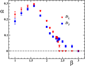
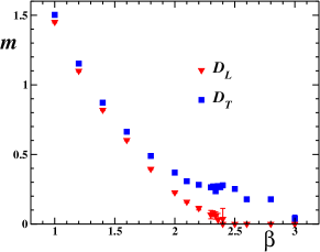
(a)	(b)

Figure 1: Fit parameters $\alpha_{L/T}$ and $m_{L/T}$ vs. $\beta$ for $D_{L}$ and $D_{T}$ formfactors (from Refs. Chernodub:2001mg ; Chernodub:2002gp ).

One can see from Figure 1(a) that the anomalous dimension for the temporal photons, $\alpha_{L}$, vanishes exactly at the point of the phase transition ($\beta_{c}=2.30(2)$ according to Ref. Chernodub:2001ws ) whereas the spatial photons do not seem to feel this transition. This is documented by $\alpha_{T}$ not vanishing at $\beta=\beta_{c}$. Similarly, a different behavior is seen for the mass parameters $m_{L}$ and $m_{T}$ as shown in Figure 1(b).

The vanishing of the parameters $\alpha_{L}$ and $m_{L}$ of $D_{L}$ at $\beta_{c}$ and beyond is clearly corroborating the finite temperature phase transition Chernodub:2001mg caused by dipole formation. The fields of the dipoles are weak at large distances and they cannot cause neither the Debye screening no-screening nor confinement. Thus the origin of the non-zero mass $m_{T}$ of the spatial photon propagator in the deconfinement phase is likely to be an artifact of the lattice simulations, more specifically, of the insufficient gauge fixing. We have checked in Ref. Chernodub:2002gp that this propagator is strongly affected by the Gribov copy problem. As we have argued in Ref. Chernodub:2002gp , the Landau gauge minimizes the total length of the Dirac strings and, in the idealized case, does not allow for closed Dirac strings (Dirac loops) to exist. However, if the Dirac loop is closed by wrapping around the torus, it is practically impossible to get rid of this gauge artifact relying only on local gauge-fixing algorithms. Gauge copies with unremoved TDL’s correspond to local minima of the gauge fixing functional. We have qualitatively noticed in Ref. Gargnano that these strings should be blamed for the unphysical behavior of $D_{T}$ in the deconfined phase if compared to $D_{L}$.

III Quantifying the effect of wrapping Dirac strings

Let us now discuss the effect of closed Dirac loops on the spatial photon propagator in a more quantitative way. As we have already mentioned, we have simulated the model at $\beta=2.6$ using a $32^{2}\times 8$ lattice. As in our previous work we have considered two possible update algorithms: one purely local one (five-hit Metropolis update alternating with a microcanonical sweep) and another which included random offers of changing the flux in one of the three directions by one unit, augmented by a Metropolis acceptance check. Finally, in order to reduce the influence of choosing between different Landau gauge-fixed copies we have performed the gauge fixing procedure 100 times on random gauge copies of the same Monte Carlo configuration ($N_{\rm copy}=100$). The evaluation of the propagator was done on the ”best” configuration corresponding to the relative maximum of the gauge functional among all $101$ gauge fixed configurations.

In our previous work Chernodub:2002gp the fit parameters which should describe the formfactor $D_{T}$ have been obtained for a number $N_{\rm copy}$ which was gradually increased, and even 100 Gribov copies were found to be insufficient for convergence. This seems to exclude the possibility to improve the result further by local gauge-fixing algorithms exclusively. The parameters for the longitudinal formfactor $D_{L}$ were found to converge already for $N_{\rm copy}\approx 10$. This explains why, for the present purpose, we kept $N_{\rm copy}=100$. Due to the asymmetry of the lattice it is relatively easy that Dirac strings are generated running around the lattice in temporal direction. We restrict ourselves to a string search in that direction in order to separate our ensemble of (locally) gauge-fixed configurations into classes according to the number of TDL’s. A Dirac loop is formed by a connected sequence of dual links carrying directed Dirac string bits $n_{{\vec{x}};\mu}^{\rm Dirac}\neq 0$. A full Dirac string is defined by penetrating a stack of Dirac plaquettes. A plaquette, say $P=P_{{\vec{x}};\mu\nu}=P_{(x_{1},x_{2},x_{3});1,2}$, is identified as one of the pierced, i.e. Dirac plaquettes if

$$n_{{\vec{x}};3}^{\rm Dirac}=\frac{1}{2\pi}[\theta_{P}]_{{\rm mod}2\pi}\,.$$ (14)

is a non-vanishing integer. Positive or negative values – usually plus or minus one – define the direction of the string bit.

The implementation of such a search, following the stack of Dirac plaquettes and counting the number of closed Dirac loops, is too time consuming in general. Deeper in the deconfined phase, it is possible to characterize a given thermalized and gauge fixed configuration by summing up the modules $N_{3}$ and the values of those integer Dirac plaquettes $I_{3}$ pointing into the third (”short”) compactified direction

$$N_{3}={\rm Integer}\left[\frac{1}{L_{3}}\sum_{x}|n_{{\vec{x}},3}^{\rm Dirac}|\right]$$ (15)

and

$$I_{3}={\rm Integer}\left[\frac{1}{L_{3}}\sum_{x}n_{{\vec{x}},3}^{\rm Dirac}\right]\,.$$ (16)

The different sectors of possible thermal Dirac loops are labelled by a number $N_{3}=0,1,\dots$ If the expected TDL’s are mainly static (i.e. already minimized in length), the quantity $N_{3}$ counts the number of those strings under the assumption that the number of monopoles is already very low (what is the case at $\beta=2.6$). In case $|I_{3}|$ coincides with $N_{3}>1$, all TDL’s have the same wrapping orientation, otherwise TDL’s with different orientation are present. With this procedure we cannot assess whether those strings are really ”at rest” on the same $(x_{1},x_{2})$ position or not, but this classification is robust enough to allow for some local dislocations of the TDL’s. The ratio

$$r_{3}=\frac{{\rm{Number\,of\,measurements\,with\,}}|I_{3}|=N_{3}}{{\rm{All\,measurements\,in\,sector\,}}N_{3}}$$ (17)

counts the fraction of such strings having the same wrapping orientation. Having identified the ”thermal Dirac loop number” $N_{3}$, we can classify a given gauge-fixed configuration according to its string content and measure the photon propagator separately in the different sectors.

In our previous Monte Carlo analysis Chernodub:2002gp we have used both local and “blended” updates, the latter including in addition to the local update adding and subtraction of fluxes, among them fluxes through the $(x_{1},x_{2})$-plane. Therefore, in the light of the string sector classification, we also have to consider the effect of the chosen Monte Carlo algorithm on this classification.

First, we have checked the dependence of the propagators on the number of thermal Dirac loops. In Figure 2

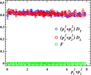
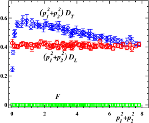
(a)	(b)
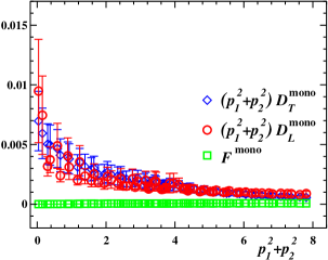
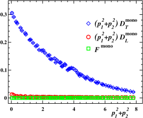
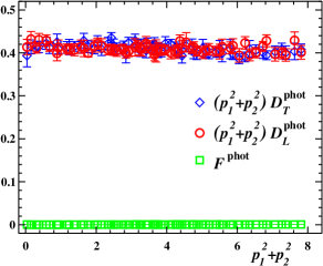
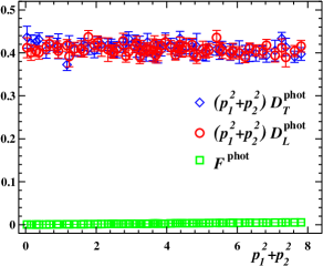
(e)	(f)

Figure 2: The formfactors $D_{L}$, $D_{T}$ and $F$ vs. spatial momentum in the sector with (left column) zero, $N_{3}=0$, and (right column) one, $N_{3}=1$, thermal Dirac loop using the local update. The total (a,b), singular (c,d) and regular (e,f) contributions are shown.

we present the formfactors $D_{L}$, $D_{T}$ and $F$ in the sectors without and with one TDL. Here we have used only the local update algorithm. One may readily notice that the total formfactor of the spatial photons $D_{T}$ shown in Figure 2(a,b) depends significantly on the number of thermal Dirac loops whereas the $D_{L}$ and $F$ formfactors are insensitive (within error bars) to that number.

A very similar effect is observed for the singular contributions to formfactors which are depicted in Figures 2(c,d). The singular contribution to the $D_{T}$ formfactor in the sector with one TDL (Figure 2(d)) is about two orders of magnitude larger than in the $N_{3}=0$ sector, shown in Figure 2(c). The singular contributions to other formfactors are not affected by the presence of TDL’s.

In order to show that the thermal Dirac loops make contributions only to the singular and mixed part of the $D_{T}$ propagator, whereas the regular part is not affected by the Dirac string, we plot in Figures 2(e,f) the regular part of the $D_{T}$, $D_{L}$ and $F$ formfactors as a function of spatial momentum. One can see that the regular contributions in the zero-loop and one-loop sectors coincide within error bars.

Qualitatively, the results in Figures 2 can be understood as follows. The fact that the regular contribution to the propagator is insensitive to the number of TDL’s is very natural since the regular part does not receive contributions from singular structures like the Dirac strings. The sensitivity of the $D_{T}$ formfactor to the number of TDL’s and the respective insensitivity of the $D_{L}$ formfactor follows from Eq. (11). Indeed, the TDL is described by a chain of the plaquettes which are perpendicular to the temporal direction. The boundary of the plaquette $\delta p[j]$ is a vector field the spatial components of which are non-zero, whereas the temporal ones are vanishing. The inverse Laplacian in Eq. (11) does not mix these components. Thus, a thermal Dirac loop may provide a contribution only to the spatial components of the gauge potential, i.e. to $D_{T}$ only. Finally, the insensitivity of the formfactor $F$ to the presence of TDL’s follows from the fact that $F$ corresponds to the longitudinal (in momentum) part of the propagator whereas the contribution from the TDL is transverse (see Eq. (11)).

In the sector without thermal Dirac loops ($N_{3}=0$) the tiny singular contribution to the propagators $D_{T}$ and $D_{L}$ can be explained as an effect of remaining monopole-antimonopole pairs which are mainly oriented in temporal direction (and/or additionally of strings in spatial direction on which we did not trigger).

So far, the results in Figures 2 were obtained from the evaluation of gauge-fixed configurations when the original ensemble was generated by exclusively local updates. We have repeated the same analysis for the blended update algorithm mentioned which includes also global changes of fluxes. On this basis, we notice that (within error bars) the results for the propagator formfactors in the individual TDL sectors are independent of whether blended updates are allowed or not.

However, the choice of the update algorithm (blended or local) influences the relative weight of the individual sectors within the gauge-fixed ensemble. Strictly speaking, the content of wrapping Dirac strings is a gauge artifact. We are only monitoring it. Only dedicated, ”big” gauge transformations would be able to remove them. For example, if global flux changes are accepted in the blended update then after applying local gauge fixing the sector with $N_{3}=\pm 1$ is slightly dominating. If a local update is applied without offering global flux changes, after local gauge fixing the $N_{3}=0$ sector is clearly the dominating one. An overview of the statistics available for this study is given in Table 1.

$N_{3}$ (Update)	$r_{3}$	$\#$ of meas. in sector $N_{3}$	$\#$ of meas. attempts
0 (local)	1.0	1191	2000
0 (blended)	1.0	767	2000
1 (local)	0.891	911	2500
1 (blended)	0.903	1115	2500
2 (local)	0.866	1912	7000
2 (blended)	0.778	974	7000
3 (local)	0.859	580	15000
3 (blended)	0.869	314	20500
4 (local)	0.895	19	600000
4 (blended)	0.931	72	600000

Table 1: Statistics for the different thermal Dirac loop sectors using local or blended update.

From this Table we can speculate that in the process of gauge fixing the local algorithm might have annihilated thermal Dirac loops of different orientation to a large extent. This is expressed by the ratio (17) which is of the order of 80 % or larger. This would correspond to a suppression of so called double Dirac loops (analogues of the mentioned DDS in four dimensions) in the configurations possessing two oppositely oriented TDL’s.

It turns our that the fit of the formfactor $D_{T}$ using the functional dependence on $p$ given in (13) works very well separately for all sectors $N_{3}=0,\dots,4$, with $\chi^{2}/d.o.f.\approx 0.5$. The corresponding fitting curves yielding $\alpha_{T}$ and $m_{T}$ separately for each $N_{3}=0,\dots,3$, are shown in Figure 3.

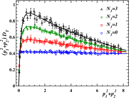
Figure 3: The total formfactor $D_{T}$ for spatial photons in the different TDL sectors, using the blended update. The data are fitted by the function (13).

The fitting parameters themselves as functions of the TDL multiplicity $N_{3}$ are shown in Figure 4 both for the local and the blended updates.

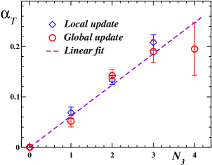
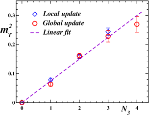
(a)	(b)
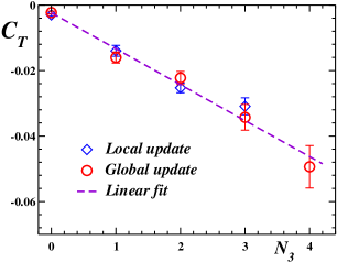
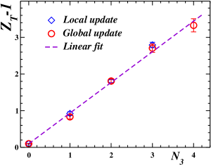
(c)	(d)

Figure 4: Fit parameters $\alpha_{T}$, $m_{T}$, $Z_{T}$ and $C_{T}$ for the $D_{T}$ formfactor vs. the number of thermal Dirac loops $N_{3}$ using data obtained with blended or local updates. The fits by Eqs. (18) are presented by dashed lines.

First we notice that the fit parameters in a given loop sector are practically independent of the update. As one can see from Table 1, our statistics for $N_{3}=4$ achieved by exclusively local updates is quite low such that we omit the corresponding points in Figures 4. We emphasize the observation that it is extremely unlikely to produce, by updates without global changes of flux, configurations which finally, after gauge fixing, end up in the sector $N_{3}=4$.

In the sector without thermal Dirac loops ($N_{3}=0$) the anomalous dimension $\alpha_{T}$, the mass parameter $m_{T}$ and the contact term parameter $C_{T}$ are consistent with zero. At the same time, the renormalization of the photon wavefunction $Z_{T}$ is very close to unity. Thus, if we would restrict ourselves to the $N_{3}=0$ sector in the propagator measurements, there is practically no difference between the $D_{L}$ and $D_{T}$ formfactors in the deconfinement phase, and we reproduce the expected behavior of a trivial free photon propagator.

In the non-zero TDL sector ($N_{3}\geqslant 1$) the parameters $\alpha_{T}$, $m_{T}$ and $C_{T}$ become non-zero, and the parameter $Z_{T}$ deviates from unity. Thus, the formfactor acquires a non-trivial momentum dependence compared to the sector without thermal Dirac loops. The dependence of the propagator parameters, $\alpha_{T}$, $m_{T}^{2}$, $Z_{T}$ and $C_{T}$, on the multiplicity of thermal Dirac loops, $N_{3}$, can be described by simple linear functions:

$$\alpha_{T}=a_{\alpha}\,N_{3}\,,\quad m_{T}^{2}=a_{m}N_{3}\,,\quad Z_{T}-1=a_{Z}N_{3}\,,\quad C_{T}=a_{C}N_{3}\,.$$ (18)

The corresponding fits are shown by the dashed lines in Figures 4. The quality of these fits is approximately the same, $\chi^{2}/d.o.f.\approx 1.5$. The proportionality coefficients are $a_{\alpha}=0.062(5)$, $a_{m}=0.0745(38)$, $a_{Z}=0.84(3)$ and $a_{C}=-0.011(1)$. We recall that all this refers to a temperature corresponding to $\beta=2.6$. We expect that in general these coefficients must depend on temperature.

IV Conclusions

We have studied the influence of thermal Dirac loops on the gauge boson propagator within the finite temperature compact $U(1)$ gauge model in three dimensions. We have used the Landau gauge and worked deep inside the deconfinement phase where monopoles are very dilute and Dirac strings are dilute as well. This allows us to unambiguously recognize the thermal Dirac loops. Wrapping Dirac strings are ubiquitous on a finite lattice. On an asymmetric lattice at high temperature they are predominantly closed along the temperature direction which is the shortest lattice direction. Although closed Dirac loops along the spatial directions (non-thermal Dirac loops) are not completely excluded, they are extremely rare and do not yield an essential contribution to the propagator $D_{T}$ in question.

Strictly speaking, in the Landau gauge Dirac strings closed due to periodic boundary conditions are artifacts of the gauge fixing, because the Landau gauge condition corresponds to the minimization of the number and length of Dirac strings Chernodub:2002gp . We have found that the presence of such thermal Dirac loops seriously affects the properties of the propagator, in the considered case those of $D_{T}$, in the deconfinement phase. The propagator formfactor corresponding to spatial photons in a sector with a non-vanishing number $N_{3}$ of TDL’s mimics a momentum dependence similar to what is known from the confinement phase, Eq. (13). The parameters, which describe the deviation from the free photon propagator, which ought to be expected in the deconfinement phase, are found clearly proportional to $N_{3}$ because we were working in dilute gas regime. An explanation of this coincidence may lie in the fact that the monopoles, which are active in the confinement phase, contribute to the propagator only indirectly, i.e. via the Dirac strings.

- (1) A. M. Polyakov, Nucl. Phys. B 120, 429 (1977).
- (2) H. R. Fiebig and R. M. Woloshyn, Phys. Rev. D 42, 3520 (1990).
- (3) Y. Hosotani, Phys. Lett. B 69, 499 (1977); V. K. Onemli, M. Tas and B. Tekin, JHEP 0108, 046 (2001).
- (4) G. Baskaran and P. W. Anderson, Phys. Rev. B 37, 580 (1998); L. B. Ioffe and A. I. Larkin, ibid. B 39, 8988 (1989); P. A. Lee, Phys. Rev. Lett. 63, 680 (1989); T. R. Morris, Phys. Rev. D 53, 7250 (1996).
- (5) M. N. Chernodub, E.-M. Ilgenfritz and A. Schiller, Phys. Rev. D 64, 054507 (2001).
- (6) N. O. Agasian and K. Zarembo, Phys. Rev. D57 (1998) 2475.
- (7) M. N. Chernodub, E.-M. Ilgenfritz and A. Schiller, Phys. Rev. Lett. 88, 231601 (2002); Nucl. Phys. Proc. Suppl. 119, 766 (2003).
- (8) M. N. Chernodub, E.-M. Ilgenfritz and A. Schiller, Phys. Lett. B 547, 269 (2002).
- (9) H. Kleinert, F. S. Nogueira and A. Sudbø Phys. Rev. Lett. 88, 232001 (2002); A. Sudbø et al., ibid. 89, 226403 (2002).
- (10) M. N. Chernodub, E.-M. Ilgenfritz and A. Schiller, Phys. Lett. B 555, 206 (2003).
- (11) M. N. Chernodub, E.-M. Ilgenfritz and A. Schiller, Phys. Rev. D 67, 034502 (2003); hep-lat/0301010.
- (12) M. N. Chernodub, E.-M. Ilgenfritz and A. Schiller, in ”Quark Confinement and the Hadron Spectrum V”, eds. N. Brambilla and A. M. Prosperi, World Scientific (2003), p. 249; e-print archive hep-lat/0301010.
- (13) V. G. Bornyakov, V. K. Mitrjushkin, M. Muller-Preussker and F. Pahl, Phys. Lett. B 317, 596 (1993); I. L. Bogolubsky, L. Del Debbio and V. K. Mitrjushkin, Phys. Lett. B 463, 109 (1999); [arXiv:hep-lat/9903015]. I. L. Bogolubsky, V. K. Mitrjushkin, M. Muller-Preussker and P. Peter, Phys. Lett. B 458, 102 (1999); S. Durr and P. de Forcrand, Phys. Rev. D 66, 094504 (2002).
- (14) V. K. Mitrjushkin, Phys. Lett. B 389, 713 (1996).
- (15) R. J. Wensley and J. D. Stack, Phys. Rev. Lett. 63, 1764 (1989).
- (16) T. DeGrand and D. Toussaint, Phys. Rev. D 22, 2478 (1980).
- (17) J. Glimm and A. Jaffe, Comm. Math. Phys. 56, 195 (1977); J. Fröhlich and T. Spencer, J. Stat. Phys. 24, 617 (1981).
- (18) M. N. Chernodub, Phys. Rev. D 63, 025003 (2001); B. L. Bakker, M. N. Chernodub and A. I. Veselov, Phys. Lett. B 502, 338 (2001).