Static potential, force, and flux-tube profile in 4D compact U(1) lattice gauge theory with the multi-level algorithm

Abstract

The long range properties of four-dimensional compact U(1) lattice gauge theory with the Wilson action in the confinement phase is studied by using the multi-level algorithm. The static potential, force and flux-tube profile between two static charges are successfully measured from the correlation function involving the Polyakov loop. The universality of the coefficient of the $1/r$ correction to the static potential, known as the Lüscher term, and the transversal width of the flux-tube profile as a function of its length are investigated. While the result supports the presence of the $1/r$ correction, the width of the flux tube shows an almost constant behavior at a large distance.

, ,

1 Introduction

There is a conjecture that (non supersymmetric) confining gauge theories in the infrared regime are related to an effective bosonic string theory. If this happens, the asymptotic behavior of the potential between static charges separated by distance $r$ is expected to be parametrized as

$$V(r)=\sigma r+\mu+\frac{\gamma}{r}+O(\frac{1}{r^{2}}).$$ (1)

Here $\sigma$ is the string tension, which characterizes the strength of the confining force of static charges, and $\mu$ denotes a constant. The third term is the zero point Casimir energy for an open bosonic string with fixed boundary. This correction is known as the Lüscher term [1] and the coefficient $\gamma$ is considered to be universal, such that it does not depend on the gauge group but only on the space-time dimension $d$ through $\gamma=-\pi(d-2)/24$. The effective bosonic string theory also predicts that the width of the field energy distribution of the flux tube diverges logarithmically as $r\to\infty$ [2]. Recent Monte Carlo simulations of various lattice gauge theories support the universality of $\gamma$ in Eq. (1) with high accuracy: the confinement phase of $Z\!\!\!Z_{2}$ lattice gauge theory (LGT) in 3D [3, 4, 5], SU(2) LGT in 3D [6, 7] and in 4D [8], SU(3) LGT in 3D [9] and in 4D [9, 10]. Moreover, in Refs. [6, 10], the spectrum of the string states have been computed, which further support the effective string description of confining gauge theories.

In this context, we are now interested in the 4D compact U(1) LGT with the Wilson action. This theory possesses a confinement phase analogous to non-Abelian gauge theories below the critical coupling $\beta<\beta_{c}\approx 1.011$ (precise value can be found in Ref. [11]). This is due to the presence of magnetic monopoles [12], which cause the dual Meissner effect like in a dual superconductor [13, 14] when electric sources are introduced in the vacuum; the electric flux is squeezed into a flux tube by the circulating monopole supercurrent, which leads to a linear rising potential between static charges. In fact, the measurements of the U(1) flux-tube profile in the confinement phase have been reported in Refs. [15, 16], which support the dual superconductor picture. To answer the questions i) whether the static potential in this theory also contain the universal correction, ii) how the width of the flux-tube profile behaves as a function of $r$, in this paper, we investigate the long range properties of the potential, force and the flux-tube profile between two static charges. Here we are going to use the Polyakov loop correlation function (PLCF: a pair of Polyakov loops separated by a distance $r$) as an external source. Contrary to the use of the Wilson loop $\langle W(r,t)\rangle$, if we use the PLCF $\langle P^{*}P(r)\rangle$, we do not need to care about the $t$ dependence of the results and can extract the the ground state easily as long as the lattice temporal extension is large enough. This is important because most of analytical predictions are given for such a ground state. However, the measurement of the PLCF in the confinement phase with large $r$ is a quite difficult task since the expectation value becomes exponentially smaller with increasing $r$. Moreover, due to the strong coupling nature of the theory, the signal-to-noise ratio is very small from the beginning. In principle, one would need enormous statistics and computation time to identify such small expectation values.

Recently, Lüscher and Weisz (LW) have proposed a multi-level algorithm for pure LGT [17] to compute the expectation value of a Wilson loop for a large size and a PLCF for large $r$ with exponentially reduced statistical errors. They noted that its algorithmic idea is essentially the same as in the multi-hit method [18] but is applied to pairs of links instead of single links. In fact, based on their algorithm they have confirmed the presence of an universal potential $\gamma/r$ in SU(3) LGT [9]. The LW algorithm is applicable to other LGTs as long as a local gauge action is simulated. The Wilson action is the easiest gauge action to adopt. The studies of 3D SU(2) LGT [6, 7] also use this algorithm. We then expect that the LW algorithm can also be applied to compact U(1) LGT, which will help to overcome its numerical difficulties. In the original work [9], although the potential and its derivatives with respect to $r$, force etc., have been of interest, we find that this is also applicable to measuring the flux-tube profile as well as the glueball mass measurements [19].

In section 2, we describe the LW algorithm for the measurements of the static potential and force from the PLCF. We also explain how to measure the flux-tube profile in this context. In sections 3 and 4, we present simulation details and the numerical results on the PLCF/potential/force and on the the flux-tube profiles, respectively, where several analyses of the data are given. The section 5 is a summary. A part of these studies has been presented at the Lattice 2003 at Tsukuba, Japan [20].

2 Numerical procedures

In this section we describe how to measure the static potential, force and flux-tube profile with the LW algorithm.

The Wilson gauge action of the compact U(1) LGT is given by

$$S[U]=\beta\sum_{m}\sum_{\mu<\nu}\left\{1-{\rm Re}\;[U_{\mu\nu}(m)]\right\}\;,$$ (2)

where $U_{\mu\nu}(m)\in U(1)$ are plaquette variables constructed from link variables $U_{\mu}(m)=\exp(i\theta_{\mu}(m))\in U(1)$. We consider the lattice volume $N_{s}^{3}\times N_{t}$, where $N_{t}$ is an even number. The four-dimensional sites are labeled by $m=(m_{s},m_{t})$ with $m_{s}=(m_{1},m_{2},m_{3})$. Periodic boundary conditions are imposed for all directions. A sequence of independent gauge field configurations, labeled by $i_{c}=1,2,\ldots,N_{c}$, are generated by using a mixture of heatbath (HB) and over-relaxation (OR) link updates as usual.

2.1 The static potential and force from the PLCF

We adopt the terminology of Ref. [17]. To measure the PLCF $\langle P^{*}P(R)\rangle$ for a charge distance $R=r/a$, we first take sub-lattice averages of the two-link correlators

$$\mathbb{T}(m;R;i)=U_{4}^{*}(m)U_{4}(m+R\;\hat{i})\;,$$ (3)

as

$$\mathbb{T}^{(2)}(m_{s},\bar{m}_{t};R;i)=[\mathbb{T}(m;R;i)\mathbb{T}(m+\hat{4};R;i)]\;,$$ (4)

where $i=1,2,3$ are possible directions of two static charges and $\bar{m}_{t}=1,3,\ldots,N_{t}-1$. The sub-lattice average is achieved by updating link variables (with a mixture of HB/OR) except for the spatial links at the time slice $\bar{m}_{t}$. We call this procedure the internal update. We repeat the internal update until reasonably stable values for $\mathbb{T}^{(2)}$ are obtained.

Then, the PLCF at a spatial site $m_{s}$ is constructed from $\mathbb{T}^{(2)}$ as

$$P^{*}P(m_{s};R;i)=P^{*}(m_{s})P(m_{s}+R\hat{i})$$ (5)

$$= {\rm Re}\;\mathbb{T}^{(2)}(m_{s},1;R;i)\mathbb{T}^{(2)}(m_{s},3;R;i)\cdots\mathbb{T}^{(2)}(m_{s},N_{t}-1;R;i)\;.$$

We take the average with respect to $m_{s}$ and $i$, which provides the value of the PLCF for $i_{c}$th configuration, $\left[P^{*}P(R)\right]_{i_{c}}$. For a schematic understanding, see Fig. 1. The desired expectation value $\langle P^{*}P(R)\rangle$ is calculated from the average of $\left[P^{*}P(R)\right]_{i_{c}}$ for $i_{c}=1,2,\ldots,N_{c}$.

Figure 1: How to construct the $[P^{*}P]_{i_{c}}$ with the LW algorithm. $[\cdots]$ denotes the sub-lattice average.

The static potential and the corresponding force are taken as (neglecting terms of $O(e^{-(\Delta E)N_{t}})$)

$$aV(R) = -\frac{1}{N_{t}}\ln\langle P^{*}P(R)\rangle\;,$$ (6)

$$a^{2}F(\bar{R}) = aV(R)-aV(R-1)\;,$$ (7)

where $\bar{R}=R-1/2$.

In the actual measurements, we have also applied the multi-hit technique [18] to the timelike link variables $U_{4}(m)$ for $R\geq 2$ before constructing the two-link correlators (3). It was further helpful to reduce the statistical errors of the PLCF within a limited CPU time. In U(1) LGT, this procedure is given by the replacement

$$U_{\mu}(m)\mapsto\frac{I_{1}(\beta|W_{\mu}(m)|)}{I_{0}(\beta|W_{\mu}(m)|)}\frac{W_{\mu}(m)}{|W_{\mu}(m)|}\;,$$ (8)

where $I_{0}$ and $I_{1}$ denote the zeroth- and first-order modified Bessel functions and $W_{\mu}(m)$ the sum of six staples around $U_{\mu}(m)$:

$$\!\!\!\!\!\!\!\!\!\!W_{\mu}(m)\!=\!\sum_{\nu\neq\mu}\Bigl{[}U_{\nu}^{*}(m\!+\!\hat{\mu})U_{\mu}(m\!+\!\hat{\nu})U_{\nu}(m)\!+\!U_{\nu}(m\!+\!\hat{\mu}\!-\!\hat{\nu})U_{\mu}(m\!-\!\hat{\nu})U_{\nu}^{*}(m)\Bigr{]}\;.$$ (9)

Some comments associated with the LW algorithm are in order. The number of the internal updates $N_{\rm iupd}$ is an optimization parameter that has to be tuned for efficient performance of the computation. If one wants to compute the force, which requires two values of the potential at different $r$, it is useful to compute all $R=1,2,\ldots,R_{\rm max}$ in one run without changing $N_{\rm iupd}$ depending on $R$, although a small number of $N_{\rm iupd}$ is enough for a short distance. This is because data among different $R$’s are highly correlated, which leads to a significant cancellation of the statistical errors in the difference [9]. Practically, one may regard not only the PLCF but also the potential and force as the primary observables and apply the jackknife analysis for the evaluation of the statistical errors.

2.2 The flux-tube profile

In order to measure the flux-tube profile, one needs to compute a correlation function of the type

$$\langle\mathcal{O}(n)\rangle_{j}=\frac{\langle P^{*}P\mathcal{O}(n)\rangle_{0}}{\langle P^{*}P\rangle_{0}}-\langle\mathcal{O}\rangle_{0}\;,$$ (10)

where $\mathcal{O}(n)$ is a local operator, $\langle\cdots\rangle_{j}$ denotes an average in the vacuum with the PLCF, and $\langle\cdots\rangle_{0}$ an average in the vacuum without such a source. For a parity-odd local operator, we do not need the second term since it gives no contribution, $\langle\mathcal{O}\rangle_{0}=0$. However, if one is interested in a parity-even local operator such as the action density $\cos\theta_{\mu\nu}(n)$, where $\theta_{\mu\nu}(n)$ is the phase of $U_{\mu\nu}(n)$, one needs to subtract out the vacuum expectation value. It is noted that to receive maximum benefit from the LW algorithm, the parity-odd local operator is preferable [19].

To measure $\langle P^{*}P\mathcal{O}(n)\rangle_{0}$ on the mid-plane between two static charges, we parameterize the position of the local operator $n$ as

$$n=m+(R/2)\hat{i}+x\hat{j}+y\hat{k}\;,$$ (11)

where $i$ is the direction of two static charges and $j-k$ specify a 2D plane perpendicular to $i$. By constructing the two-link-local-operator correlators

$$\mathbb{O}(m;n;R;i)=U_{4}^{*}(m)U_{4}(m+R\hat{i})\mathcal{O}(n)\;,$$ (12)

we compute sub-lattice averages of the correlation function

$$\mathbb{TO}^{(2)}(m_{s},\bar{m}_{t};n;R;i)=[\mathbb{T}(m;R;i)\mathbb{O}(m+\hat{4};n;R;i)]\;.$$ (13)

Combining $\mathbb{TO}^{(2)}$ and $\mathbb{T}^{(2)}$ in Eq. (4), we obtain the PLCF involving a local operator at site $m_{s}$ as

$$\!\!\!\!\!\!\!\!\!\!P^{*}P\mathcal{O}(m_{s};x,y;R;i)$$

$$\!\!\!\!\!\!\!\!\!\!=\frac{1}{(N_{t}/2)}{\rm Re}\;\Biggl{\{}\mathbb{TO}^{(2)}(m_{s},1;n;R;i)\mathbb{T}^{(2)}(m_{s},3;R;i)\cdots\mathbb{T}^{(2)}(m_{s},N_{t}-1;R;i)+$$

$$\cdots+\mathbb{T}^{(2)}(m_{s},1;R;i)\mathbb{T}^{(2)}(m_{s},3;R;i)\cdots\mathbb{TO}^{(2)}(m_{s},N_{t}-1;n;R;i)\Biggr{\}}\;.$$ (14)

The average with respect to $m_{s}$ and $i$ provides $\left[P^{*}P\mathcal{O}(x,y;R)\right]_{i_{c}}$. For a schematic understanding, see Fig. 2. We repeat the same procedure as for the PLCF to get the final expectation value $\langle P^{*}P\mathcal{O}(x,y;R)\rangle$.

Figure 2: How to construct $[P^{*}P\mathcal{O}]_{i_{c}}$ with the LW algorithm. $[\cdots]$ denotes the sub-lattice average and the square represents a local operator.

As a local operator, we use the electric field operator (parity odd) as

$$\mathcal{O}_{E}(n)=i\bar{\theta}_{\mu\nu}(n)=i(\theta_{\mu\nu}(n)-2\pi n_{\mu\nu}(n))\;,$$ (15)

where $\theta_{\mu\nu}(n)\in[-4\pi,4\pi]$ and $n_{\mu\nu}(n)\in[0,\pm 1,\pm 2]$ is the modulo $2\pi$ of $\theta_{\mu\nu}(n)$, which corresponds to the magnetic Dirac string. Hence, one has $\bar{\theta}_{\mu\nu}(n)\in[-\pi,\pi]$. Moreover, we use the monopole current operator (parity odd) to detect the circulating monopole supercurrent as

$$\mathcal{O}_{k}(\tilde{n})=2\pi ik_{\mu}(\tilde{n})\;.$$ (16)

Here $k_{\mu}$ is defined as the boundary of the magnetic Dirac string [12] as

$$k_{\mu}(\tilde{n})=\frac{1}{2}\varepsilon_{\mu\nu\alpha\beta}\partial_{\nu}n_{\alpha\beta}(n+\hat{\mu})\qquad\in[0,\pm 1,\pm 2]\;.$$ (17)

$\tilde{n}$ denotes the dual site $n+(\hat{1}+\hat{2}+\hat{3}+\hat{4})/2$.

We have chosen these local operators because of the possibility to relate the U(1) flux tube and the classical flux-tube solution of the dual Ginzburg-Landau (DGL) theory. In the DGL theory, the circulating monopole supercurrent induces the solenoidal electric field through the dual Ampère law, which plays a role in cancelling the Coulombic field induced by static charges at a distant place. In this sense the measurement of the monopole current profile is useful to judge whether the total electric flux is indeed squeezed or not. In Appendix A, we show a numerical evidence of such a cancellation mechanism of the electric flux inside the U(1) flux tube. We may call this the composite structure of the U(1) flux tube.

Note that the definitions of the electric field and monopole current operators are not unique. For instance, Cheluvaraja et al. [21], have proposed an alternative definition to satisfy the the Maxwell equations at finite lattice spacing. It would also be interesting to study how the measured flux-tube profiles change with their operators.

3 Numerical results : Static potential and force from the PLCF

In this section, we first present the simulation details associated with the LW algorithm for the measurements of the potential and force from the PLCF, and then, we show the corresponding numerical results. Some analyses are also performed for the potential and force; the potential is fitted with several ansätze. The behavior of the force is compared with the function derived from Eq. (1).

3.1 Simulation details

We use a $16^{4}$ lattice. The $\beta$ values, the number of internal updates $N_{\rm iupd}$, the number of configurations $N_{\rm conf}$, details of one Monte Carlo update (HB/OR), and the range of measured distance between static charges $r/a$, are summarized in Table 1. Although we have not checked the finite volume effect, as we will see later, our lattice volume itself is reasonably large even near the phase transition point: $(\sim 3.5r_{0})^{4}$ at $\beta=1.01$. In addition to this, we restrict ourselves to measure the potential up to $r/a=6$.

Table 1: Parameter setting

$\beta$	$N_{\rm iupd}$	$N_{\rm conf}$	HB/OR	$r/a$ range
0.981	10000	1050	1 / 3	1–6
0.991	80001	1250	1 / 3	1–6
1.001	50001	2000	1 / 3	1–6
1.005	30001	2400	1 / 5	1–6
1.011	10001	3200	1 / 5	1–6

In Fig. 3, we show an example how we have optimized $N_{\rm iupd}$ depending on $\beta$. This plot shows a typical behavior of a PLCF at $\beta=0.98$ for one configuration $[P^{*}P(r/a)]$ as a function of $N_{\rm iupd}$. This figure tells us that, for instance, if we are interested in up to $r/a=4$, $N_{\rm iupd}=1000$ would be enough. However, if $r/a=6$ is of interest, we may need to take $N_{\rm iupd}>8000$.

Figure 3: Typical behavior of $[P^{*}P]$ for various $r$ at $\beta$ = 0.98 as a function of $N_{\rm iupd}$. When $N_{\rm iupd}$ is not sufficient, $[P^{*}P]$ often takes negative values during the internal update, typically for large $r$, where lines are broken.

3.2 Static potential and force from the PLCF

In Table 2, we summarize the expectation values of the PLCF, potential and force for all $\beta$ values measured. Note that it is possible to identify signals of the PLCF even when $\langle P^{*}P\rangle=10^{-3}\sim 10^{-16}$ with the $1\sigma$ error varying from 0.4 to 8 %.

One may think that the investigation of the second derivative of the potential as in Refs. [6, 9] for the direct identification of the coefficient of $1/r$ potential is also interesting. However we have not succeeded to get reliable data for this. The result was strongly dependent on the definition of the lattice second derivative. This may be due to the reason that in U(1) LGT the rotational invariance is not well-recovered compared to non-Abelian gauge theories even near the critical coupling.

Table 2: The PLCF, static potential and force.

$\beta$	$r/a$	$\langle P^{*}P(r/a)\rangle$	$aV(r/a)$	$\bar{r}/a$	$a^{2}F(\bar{r}/a)$
0.981	1	1.799(3)11$\times\;10^{-4\phantom{1}}$	0.5389(1)1	1.5	0.4080(3)1
	2	2.627(14)1$\times\;10^{-7\phantom{1}}$	0.9470(3)1	2.5	0.3439(5)1
	3	1.072(14)1$\times\;10^{-9\phantom{1}}$	1.2909(8)1	3.5	0.3150(6)1
	4	6.96(15)11$\times\;10^{-12}$	1.6058(14)	4.5	0.3024(12)
	5	5.54(17)11$\times\;10^{-14}$	1.9083(19)	5.5	0.3003(52)
	6	4.77(35)11$\times\;10^{-16}$	2.2086(59)
0.991	1	3.186(6)11$\times\;10^{-4\phantom{1}}$	0.5032(1)1	1.5	0.3562(3)1
	2	1.067(7)11$\times\;10^{-6\phantom{1}}$	0.8594(4)1	2.5	0.2872(4)1
	3	1.080(14)1$\times\;10^{-8\phantom{1}}$	1.1466(8)1	3.5	0.2585(7)1
	4	1.733(37)1$\times\;10^{-10}$	1.4051(14)	4.5	0.2474(12)
	5	3.35(13)11$\times\;10^{-12}$	1.6525(24)	5.5	0.2444(40)
	6	7.01(62)11$\times\;10^{-14}$	1.8970(59)
1.001	1	6.507(11)1$\times\;10^{-4\phantom{1}}$	0.4586(1)1	1.5	0.2920(2)1
	2	6.086(27)1$\times\;10^{-6\phantom{1}}$	0.7506(3)1	2.5	0.2193(5)1
	3	1.825(18)1$\times\;10^{-7\phantom{1}}$	0.9699(6)1	3.5	0.1907(14)
	4	8.66(16) $\times\;10^{-9\phantom{1}}$	1.1606(12)	4.5	0.1797(27)
	5	4.94(22)11$\times\;10^{-10}$	1.3404(20)	5.5	0.1791(35)
	6	3.00(23)11$\times\;10^{-11}$	1.5195(45)
1.005	1	1.045(2)11$\times\;10^{-3\phantom{1}}$	0.4290(1)	1.5	0.2504(2)1
	2	1.902(10)1$\times\;10^{-5\phantom{1}}$	0.6794(3)	2.5	0.1770(4)1
	3	1.121(10)1$\times\;10^{-6\phantom{1}}$	0.8565(7)	3.5	0.1498(6)1
	4	1.027(21)1$\times\;10^{-7\phantom{1}}$	1.0063(13)	4.5	0.1389(12)
	5	1.136(42)1$\times\;10^{-8\phantom{1}}$	1.1452(22)	5.5	0.1350(35)
	6	1.42(11)11$\times\;10^{-9\phantom{1}}$	1.2802(52)
1.011	1	2.152(8)11$\times\;10^{-3\phantom{1}}$	0.3839(2)1	1.5	0.1882(3)1
	2	1.061(10)1$\times\;10^{-4\phantom{1}}$	0.5720(4)1	2.5	0.1150(3)1
	3	1.687(24)1$\times\;10^{-5\phantom{1}}$	0.6871(7)1	3.5	0.0891(5)1
	4	4.076(79)1$\times\;10^{-6\phantom{1}}$	0.7762(12)	4.5	0.0784(9)1
	5	1.180(37)1$\times\;10^{-6\phantom{1}}$	0.8546(15)	5.5	0.0755(27)
	6	3.79(22)11$\times\;10^{-7\phantom{1}}$	0.9301(45)

3.3 Analysis

In this subsection, in order to see the presence/absence of the universal $\gamma/r$ correction and of more higher order corrections to the static potential, we fit the static potential assuming the several explicit forms which are close to Eq. (1):

$$V_{1}(r)=\sigma r+\mu+\frac{C}{r}\;,$$ (18)

$$V_{2}(r)=\sigma r+\mu+\frac{\gamma}{r}\;,$$ (20)

$$V_{3}(r)=\sigma r+\mu+\frac{\gamma}{r}\left(1+\frac{b}{r}\right)\;,$$

where $\gamma=-\pi/12\sim 0.262$. The form of $V_{3}$ is motivated by Ref. [9].

Before carrying out the fitting, the PLCF has been averaged in bins over intervals between 50 and 160 time units (representing 5000 and 16000 iterations) depending on $\beta$ values to reduce the autocorrelation. The potential has been computed from the nested PLCF. For each fitting function, the means of the fitting parameters have been determined from the minimum of the $\chi^{2}$ which is defined with the covariance matrix so as to take into account the correlation among different $r$’s. The errors of the fitting parameters have been estimated from the distribution of the jackknife samples of the fitting parameters. The fit range has been fixed so that the mean is consistent with that evaluated by using only the diagonal part of the covariance matrix.

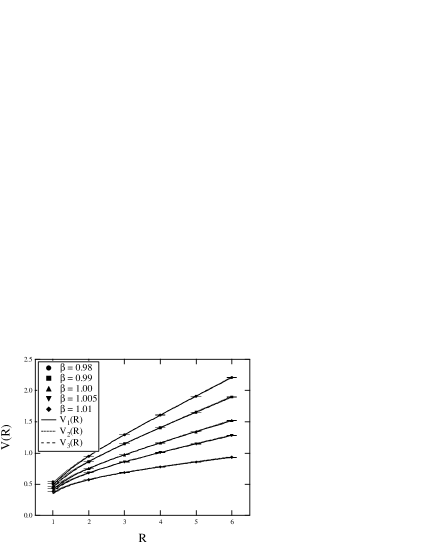
The fitting results are summarized in tables 3, 4 and 5. In Fig. 6 we have plotted the potential and the various fitting curves. As seen from this figure all curves are on the data and practically indistinguishable from each other apart from the point $R=1$, which lies outside of our fitting range. In all cases the orders of the $\chi^{2}/N_{\rm DF}$ are one or smaller than one. The coefficient $C$ obtained from $V_{1}(r)$ is slightly different from the theoretical value of $\gamma$, but not by much. However this maybe due to the existence of the Coulombic $1/r$ potential in the current fitting region. An indication of this is seen in the fit by the potential $V_{2}(r)$ where we have had to drop the point $R=2$. $V_{3}(r)$ gives a better fit, but of course it also contains an extra parameter.

At this stage, one may wonder about the relevance of $1/r$ term at long distances, since all investigated types of the function fit the potential very well. To test this we have fitted the potential with the simple form $V_{4}(r)=\sigma r+\mu$ with $r=[3,6]$ and compared with the result of $V_{2}$. It turned out that the fit was distinctly worse; the $\chi^{2}$ became 10 $\sim$ 20 times larger than that of $V_{2}$ and the means were not consistent with that determined from the use of the diagonal part of the covariance matrix.

To compare the fit results among different $\beta$ values, we introduce a scale $r_{0}$ based on Sommer’s relation $F(r_{0})r_{0}^{2}=1.65$ [22]. We have found $r_{0}/a=2.13$, 2.37, 2.83(1), 3.28(1), 4.60(3) for $\beta=0.98$, 0.99, 1.00, 1.005 and 1.01, respectively. For first two $\beta$ values there were no error at this order. Using $r_{0}$, we plot $\sigma r_{0}^{2}$ from $V_{1}$, $V_{2}$ and $V_{3}$ as a function of $\beta$ in Fig. 5. The bottom axis corresponding to $V_{1}$ and $V_{3}$ are slightly shifted in the plot to distinguish them from each other. We see slight differences among the string tensions for different ansätze of the potential. The string tensions at $\beta=$0.98 and 0.99 show a good scaling behavior with respect to $r_{0}$. For $\beta>1.00$, $\sigma_{i}r_{0}^{2}$ start to grow, which suggests that the approach to the phase transition point of the string tensions and $r_{0}$ are different. In Fig. 5, we plot $b/r_{0}$ against $\beta$, where $b$ is a coefficient of the $1/r^{2}$ potential in Eq. (20). It is interesting to find that at $\beta=$0.98 and 0.99, $b/r_{0}$ seems to be saturated. As $\beta$ increases, however, it falls down to zero. Since for large $\beta$ we can look at only the short range of the potential, this result may suggest that $b$ is irrelevant for such a range.

We then show the potential for all $\beta$ as a function of $r/r_{0}$ in Figs. 8. To subtract the constant $\mu$ in the potential plot, we have used the value obtained by the $V_{1}$ fit. We find that the potential beautifully falls onto one curve except for the data from $\beta=1.01$. The reason for this exception can be understood from Fig. 5, which shows that the string tension $\sigma r_{0}^{2}$ grows as the $\beta$ approaches to the phase transition point. We remark that the result was insensitive to the choice of the potential form used in the fit (corresponding figure from the $V_{2}$ fit is found in Ref. [20]).

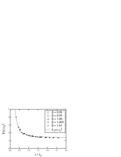
In Fig. 8, we plot the force for all $\beta$ as a function of $r/r_{0}$ and the expected function from the potential $V_{2}$: $F_{2}(r)\equiv dV_{2}(r)/dr=\sigma-\gamma/r^{2}$. It should be noted that this function contains no fitting parameter, since Sommer’s relation gives a fixed value for the string tension $\sigma r_{0}^{2}=1.65-\pi/12\sim 1.39$. We find that the general behavior of the force data seems to be described by this function. Although there are slight differences between the curve and the data at long distance, we consider that this result supports the universality of $\gamma/r$ correction to the static potential. To make a more precise statement, however, one has to control various systematic effects which enter in this analysis, for instance, the contribution of $1/r^{2}$ force which originates from the Coulombic electric field (partially discussed in Appendix A), and the possibility of higher order corrections to the static potential, which are not universal and vary from theory to theory. Surprisingly, another feature in common with non-Abelian gauge theories [23] is that this function also fits the data down to relatively short distance to $r/r_{0}\sim 0.3$. For this, there is as yet no explanation.

Table 3: Potential fit by $V_{1}(r)=\sigma r+\mu+\frac{C}{r}$.

$\beta$	$\sigma a^{2}$	$\mu a$	$C$	fit range ($r/a$)
0.981	0.286(1)	0.546(5)	$-$0.344(6)	2$-$6
0.991	0.230(1)	0.573(4)	$-$0.346(4)	2$-$6
1.001	0.162(1)	0.598(3)	$-$0.342(3)	2$-$6
1.005	0.122(1)	0.597(3)	$-$0.326(3)	2$-$6
1.011	0.0649(5)	0.595(1)	$-$0.305(1)	2$-$6

Table 4: Potential fit by $V_{2}(r)=\sigma r+\mu+\frac{\gamma}{r}$ with $\gamma=-\pi/12$.

$\beta$	$\sigma a^{2}$	$\mu a$	fit range ($r/a$)
0.981	0.294(1)	0.497(2)	3$-$6
0.991	0.238(1)	0.521(2)	3$-$6
1.001	0.171(1)	0.545(1)	3$-$6
1.005	0.130(1)	0.554(1)	3$-$6
1.011	0.0709(8)	0.565(1)	3$-$6

Table 5: Potential fit by $V_{3}(r)=\sigma r+\mu+\frac{\gamma}{r}\left(1+\frac{b}{r}\right)$ with $\gamma=-\pi/12$.

$\beta$	$\sigma a^{2}$	$\mu a$	$b/a$	fit range ($r/a$)
0.981	0.290(1)	0.517(4)	0.281(23)	2$-$6
0.991	0.233(1)	0.543(3)	0.289(15)	2$-$6
1.001	0.166(1)	0.567(2)	0.267(9)	2$-$6
1.005	0.126(1)	0.572(2)	0.208(10)	2$-$6
1.011	0.0667(5)	0.578(1)	0.138(5)	2$-$6

Figure 4: String tensions as a function of $\beta$. $\sigma$ corresponding to $V_{i}$ are denoted by $\sigma_{i}$. The bottom axis for $\sigma_{1}$ and $\sigma_{3}$ are slightly shifted to distinguish each other.

Figure 5: $b/r_{0}$ as a function of $\beta$ (see, $V_{3}(r)$ in Eq. (20)).

Figure 6: Potentials for various $\beta$ vs. the fitting curves

Figure 7: Static potential as a function of $r/r_{0}$. Constant $\mu$ is determined by $V_{1}$ fit.

Figure 8: Force as a function of $r/r_{0}$. The dashed line corresponds to $F_{2}(r)=dV_{2}(r)/dr=\sigma-\gamma/r^{2}$ with $\sigma=(1.65-\pi/12)/r_{0}^{2}$.

4 Numerical results : Flux-tube profile

In this section, we show numerical results on the flux-tube profile. We then investigate how the width of the flux tube behaves as a function of $r$ based on the DGL analysis.

4.1 Simulation details

The $\beta$ values, the lattice volume, and details of one Monte Carlo update (HB/OR) are the same as the measurement of the PLCF. Since in this case we do not compute derivatives with respect to $r$, we have changed $N_{\rm iupd}$ depending on $r$ in order to achieve a reasonable performance. The number of $N_{\rm iupd}$ is summarized in Table 6. We have measured the profile on the mid-plane between charges as described in subsection 2.2. In order to compare the profile among different $\beta$’s and $r$’s easily, we take the cylindrical average of the 2D profile; we define the radius $\rho=\sqrt{x^{2}+y^{2}}$ and the azimuthal angle around $z$ axis as $\varphi=\tan^{-1}(y/x)$.

Table 6: The number of $N_{\rm iupd}$ for the measurement of the flux-tube profile. We gave up the profile measurement for $r/a=6$ at $\beta=0.98$ because of a practical reason.

$\beta$	$r/a$	$N_{\rm iupd}$	$r/a$	$N_{\rm iupd}$	$r/a$	$N_{\rm iupd}$	$r/a$	$N_{\rm iupd}$
0.981	3	200	4	1000	5	8000	6	$---$
0.991	3	200	4	1000	5	5000	6	8000
1.001	3	200	4	1000	5	3000	6	5000
1.005	3	200	4	1000	5	2000	6	3000
1.011	3	200	4	1000	5	1000	6	1000

4.2 Flux-tube profile

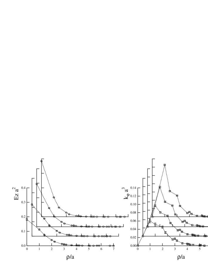
We show the profiles of electric field and monopole current in Figs. 9 – 13. The number of configurations is $N_{c}=300$ for all data. The investigated ranges are $r/r_{0}=0.469-2.35$ at $\beta=0.98$, $r/r_{0}=0.422-2.53$ at $\beta=0.99$, $r/r_{0}=0.353-2.12$ at $\beta=1.00$, $r/r_{0}=0.305-1.83$ at $\beta=1.005$ and $r/r_{0}=0.217-1.30$ at $\beta=1.01$. At glance we find that all data are clean enough, which allow us to identify the profile.

For all $\beta$ values we find a tendency that as $r$ increases, the peak of the electric field at $\rho\sim 0$ decreases and the strong peak of the monopole current profile for a small $\rho$ disappears. This feature can be understood as follows. For a small $r$, the mid-plane is close to the static charges so that the Coulombic electric field contribution is still large. In order to cancel such a strong electric field as much as possible, the monopole supercurrent must be high, which is indicated by the strong peak in Figs 9 – 13. For larger $r$ the Coulombic field is weaker in the middle and consequently the peak of the monopole current is also weaker. It is interesting that although the rotational invariance does not hold for the monopole current profile, especially for small $r$, it is effectively restored as $r$ increases.

Figure 9: Profiles of the electric field (left) and of the monopole current (right) for $r/a=$3, 4, 5 at $\beta=0.98$.

Figure 10: The same plot as in Fig. 9 at $\beta=0.99$.

Figure 11: The same plot as in Fig. 9 at $\beta=1.00$.

Figure 12: The same plot as in Fig. 9 at $\beta=1.005$.

Figure 13: The same plot as in Fig. 9 at $\beta=1.01$.

4.3 Analysis

In this subsection, we investigate how the width of the flux-tube profile depends on $r$ based on the DGL analysis. In particular, we pay attention to the data for $r/a=5$. Corresponding flux-tube lengths are $r/r_{0}=1.09\sim 2.35$. The number of configuration used for this analysis is $N_{\rm conf}=400$, 500, 700, 900 and 1200 for $\beta=0.98$, 0.99, 1.00, 1.005 and 1.01, respectively. We have increased $N_{\rm conf}$ for larger $\beta$ values to compensate the enhancement of statistical errors due to the smaller lattice spacings when the reference scale is introduced.

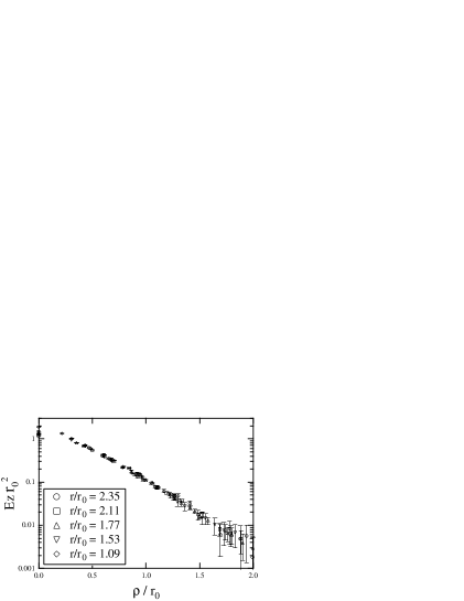
Before the analysis, let us put all profiles into one figure by introducing the Sommer scale $r_{0}$. In Figs. 15 and 15, we show the profiles of the electric field and of the monopole current, respectively. We find that the tail of the electric field profile $(\rho/r_{0}>0.4)$ seems to fall into one curve, indicating its $r$ independence. Moreover, although the monopole current profile shows squeezed shape for small $r$, it becomes wider as increasing $r$ and seems to converge again into one curve. Therefore, in the following DGL analysis we particularly pay attention to the tail behavior of the profiles.

We briefly describe the DGL theory and the classical flux-tube solution used for this analysis. The DGL Lagrangian density is given by

$$\mathcal{L}_{DGL}=-\frac{1}{4}(\partial_{\mu}B_{\nu}-\partial_{\nu}B_{\mu}-e{}^{*\!}\Sigma_{\mu\nu})^{2}\!+\!|(\partial_{\mu}\!+\!igB_{\mu})\chi|^{2}\!-\!\lambda(|\chi|^{2}\!-\!v^{2})^{2}\;,$$ (21)

where $B_{\mu}$ and $\chi=\phi e^{i\eta}$ $(\phi,\eta\in\Re)$ are the dual gauge field and the monopole field. $\Sigma_{\mu\nu}$ describes an external electric Dirac string sheet, which is bounded by the electric current $\partial_{\mu}\Sigma_{\mu\nu}=j_{\nu}$. This singularity is responsible for the location and length of the flux tube, which determines the singular part of the dual gauge field [24]. The masses of the dual gauge boson and monopole can be expressed as $m_{B}=\sqrt{2}gv$ and $m_{\chi}=2\sqrt{\lambda}v$, respectively. The inverses of these masses are corresponding to the penetration depth and coherence length, which characterize the width of the flux tube. Note that the electric coupling $e$ and the dual gauge coupling $g$ satisfy the Dirac quantization condition $eg=2\pi$. We consider a translational invariant flux tube along the $z$ axis by parameterizing the system with cylindrical coordinate $(\rho,\varphi,z)$. As mentioned, due to the Dirac string $\Sigma_{\mu\nu}$ in the dual field strength, the dual gauge field consists of a regular and a singular parts as $B_{\mu}=B_{\mu}^{\rm reg}+B_{\mu}^{\rm sing}$. For the given system, each part is reduced to $\mbox{\boldmath$B$}^{\rm reg}=\tilde{B}(\rho)/\rho\;\mbox{\boldmath$e$}_{\varphi}$ and $\mbox{\boldmath$B$}^{\rm sing}=-1/(g\rho)\;\mbox{\boldmath$e$}_{\varphi}$. The field equations for $\tilde{B}(\rho)$ and $\phi(\rho)$ are then given by

$$\frac{d}{d\rho}\left(\frac{1}{\rho}\frac{d\tilde{B}}{d\rho}\right)-2g\phi^{2}\left(\frac{g\tilde{B}-1}{\rho}\right)=0\;,$$ (22)

$$\frac{d^{2}\phi}{d\rho^{2}}+\frac{1}{\rho}\frac{d\phi}{d\rho}-\left(\frac{g\tilde{B}-1}{\rho}\right)\phi-2\lambda\phi(\phi^{2}-v^{2})=0\;.$$ (23)

The second term of the first equation is identified as the azimuthal monopole current $\mbox{\boldmath$k$}=k(\rho)\mbox{\boldmath$e$}_{\varphi}$ with $k(\rho)=-2g\phi^{2}(g\tilde{B}-1)/\rho$. One can solve the field equations analytically at large radius $\rho$ where $\phi\sim v$. In such region, the second equation provides the boundary condition of $\tilde{B}$ as $\tilde{B}\to 1/g$. By writing $\hat{\rho}=m_{B}\rho$ and $\tilde{B}=1/g-\hat{\rho}K(\hat{\rho})$, the first equation can be rewritten as

$$\frac{d^{2}K}{d\hat{\rho}^{2}}+\frac{1}{\hat{\rho}}\frac{dK}{d\hat{\rho}}-\left(1+\frac{1}{\hat{\rho}^{2}}\right)K=0\;.$$ (24)

The solution is the first-order modified Bessel function $K=K_{1}(\hat{\rho})$. For large $\rho$ it behaves as $K_{1}(\hat{\rho})\sim\sqrt{\frac{\pi}{2\hat{\rho}}}e^{-\hat{\rho}}$. Using this, one finds the solution for the electric field and the monopole current as

$$E_{z}(\hat{\rho})=\frac{1}{\rho}\frac{d\tilde{B}}{d\rho}=m_{B}^{2}K_{0}(\hat{\rho})\;,$$ (25)

$$k(\hat{\rho})=m_{B}^{3}K_{1}(\hat{\rho})\;.$$ (26)

We use these functions to find $m_{B}$. However, we must keep in mind that this solution is applicable only the region where the system is translational invariant and the monopole field has a vacuum expectation value $\phi\sim v$.

We have employed a similar fitting procedure as used in the potential fit. Before carrying out the fitting, the $\langle P^{*}P\mathcal{O}\rangle$, where $\mathcal{O}$ denotes a local operator, and $\langle P^{*}P\rangle$ have been averaged in bins over intervals between 20 and 40 time units (representing 2000 and 4000 iterations) depending on $\beta$ values to reduce the autocorrelation. Then, the cylindrical profile composed only from the on-axis data has been computed. The mean of the dual gauge boson mass has been determined from the minimum of $\chi^{2}$ defined with the diagonal part of the covariance matrix, since the correlation among different $\rho$’s was not significant, which may be due to the cylindrical averaging. The error has been estimated from the distribution of the jackknife samples of the fitting parameters. The fit range has been fixed so that the mean and/or the order of $\chi^{2}$ is stable against the change of the fit range.

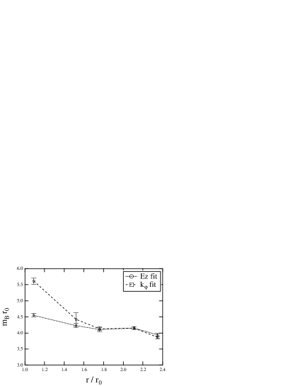
In Table 7, we summarize the result. The minimum radii which satisfy the above condition are found to be $\rho_{\rm min}/a=3$ for $\beta=0.98$ and 0.99, $\rho_{\rm min}/a=4$ for $\beta=1.00$ and 1.005, and $\rho_{\rm min}/a=5$ for $\beta=$1.01. In Fig. 16, we plot $m_{B}r_{0}$ as a function of $r/r_{0}$. We find that while the mass extracted from the $k_{\varphi}$ fit for small $r$ is larger than that from $E_{z}$ fit, it approaches $E_{z}$’s result with increasing $r$. Basically, if the ansatz for the DGL flux-tube solution (translational invariance along $z$ axis and $\phi\sim v$) is valid, the masses extracted from $E_{z}$ and those from $k_{\varphi}$ fits should coincide with each other. In this sense we should take only the result for $r/r_{0}\geq 1.77$ seriously. In fact, for short distances $k_{\varphi}$ cannot be translational invariant, because it is responsible for the solenoidal electric field inside a flux tube, which cancels the Coulombic field at large $\rho$ region (see, Appendix A). We find that the mass is stable around $m_{B}r_{0}\sim 4.0$. If the width of the flux tube diverges according to the prediction of the effective bosonic string theory, the dual gauge boson mass, identified within this analysis, should go to zero (penetration depth goes to infinity). However, we have observed an almost constant behavior of the width of the flux tube in this range. Whether a logarithmic growth of the width is hidden in our data, especially for the data at $r/r_{0}=2.35$, is however difficult to say.

Finally, we would like to discuss further the detailed fit to investigate all the three parameters in the DGL theory. We have performed the full range profile fit (whole $\rho$ region but only the on-axis data) using the finite length flux-tube solution obtained numerically within the 3D lattice discretized DGL theory as in Ref. [25]. Here, both the electric field and the monopole current profiles have been fitted simultaneously, where the diagonal part of the covariance matrix has been taken into account to define the $\chi^{2}$. The procedure to estimate the error has been the same as above. We have found, however, a tendency that this method cannot reliably be applicable for $\beta=0.98-1.005$, where the fine structure of the monopole current around the peak is not clear due to the large lattice spacing. In these cases, we could not identify the minimum of $\chi^{2}$ within the three parameter space, especially along the axis of the monopole mass. Although the dual gauge coupling has been almost a constant $\beta_{g}\sim 0.06$, the dual gauge boson mass and the monopole mass have been correlated to each other. The problem is that many sets of mass parameters have reproduced the profile well and due to this we could not find an unique set of parameters. In fact, for instance, as seen in Fig. 3 of Ref. [26], the monopole mass is responsible for the shape of the monopole current profile in small $\rho$ region, while the dual gauge boson mass that in large $\rho$ region. Only the monopole current profile at $\beta=1.01$ (see, Fig. 13 or Fig. 15 at $r/r_{0}=1.09$) has the peak at $\rho/a=2>1$. In this case we could find a minimum of $\chi^{2}$ and the parameters were found to be $\beta_{g}=0.061(2)$, $m_{B}a=0.59(2)$ and $m_{\chi}a=0.59(6)$. Taking into account the fact that the lattice spacing is still large at $\beta=1.01$, we may say that these masses are consistent with the glueball masses in the axial-vector and scalar channels given in Ref. [19].

Figure 14: Profiles of the electric field from different $r$.

Figure 15: Profiles of the monopole current from different $r$.

Table 7: The dual gauge boson mass extracted from the fit.

$\beta$	$m_{B}a$	fit range ($\rho/a$)
0.981($E_{z}$)	1.85(2)	3–6
0.981($k_{\varphi}$)	1.81(2)	3–6
0.991($E_{z}$)	1.75(2)	3–6
0.991($k_{\varphi}$)	1.75(2)	3–6
1.001($E_{z}$)	1.45(2)	4–6
1.001($k_{\varphi}$)	1.46(2)	4–6
1.005 ($E_{z}$)	1.29(2)	4–6
1.005 ($k_{\varphi}$)	1.35(6)	4–6
1.011($E_{z}$)	0.990(11)	5–6
1.011($k_{\varphi}$)	1.22(2)	5–6

Figure 16: Dual gauge boson mass extracted from the fit as a function of $r$.

5 Summary

We have successfully simulated the Wilson gauge action of 4D compact U(1) lattice gauge theory on a $16^{4}$ lattice at $\beta=$ 0.98, 0.99. 1.00, 1.005 and 1.01 (confinement phase) by using the multi-level algorithm.

First, we have measured the static potential and force between two static charges from the Polyakov loop correlation function (PLCF) up to the distance $r_{\rm max}/r_{0}=2.82$. It was possible to identify the PLCF which take values from $10^{-3}$ to $10^{-16}$ within $10$ % error. We have analyzed the potential and force by fitting with several ansätze and by comparing with Eq. (1) up to $O(1/r^{2})$ corrections, $F=dV/dr=\sigma-\gamma/r^{2}$. We have found that the potential ansatz including $\gamma/r$ describes the data well and the force is consistently described by such a function, which have supported the universality of the $\gamma/r$ correction to the static potential. Remarkably, we have also found that the function $F=\sigma-\gamma/r^{2}$ fits the force data down to relatively short distances $r/r_{0}\sim 0.3$, which is in common with non-Abelian gauge theories.

Secondly, we have measured the U(1) flux-tube profile (the electric field and the monopole current) via the PLCF for the distances $r/r_{0}=0.217-2.35$. We have investigated the width of the flux-tube profile as a function of $r$ based on the dual Ginzburg-Landau (DGL) analysis; we have fitted the tail (large $\rho$ region) of the U(1) flux-tube profile by the classical flux-tube solution of the DGL theory and have extracted the dual gauge boson mass $m_{B}$, whose inverse characterizes the width of the flux tube. We have found that the mass is almost constant for larger $r$ as $m_{B}r_{0}\sim 4.0$, which indicates that the width remains constant in the range $r/r_{0}=1.77-2.35$. If we suppose that the width grows logarithmically as predicted by the string model, the question may be whether we can identify such a behavior within the limited range of $r$. This would require a further detailed investigation especially for the range $r/r_{0}>1.77$.

Appendix A composite structure of the U(1) flux tube

In this appendix, we show the numerical evidence of the composite structure of the U(1) flux tube. This is possible by applying the Hodge decomposition to the external source to identify its monopole and photon related parts and by measuring the corresponding profiles. Unfortunately, since the Hodge decomposition requires the lattice Coulomb propagator (see, Eq. (28)), which spoils the locality of the operator, we cannot use the LW algorithm here. Thus, we measure the flux-tube profile induced by the Wilson loop with a small size as an external source instead of a PLCF to get a clear signal. How to decompose the Wilson loop into the monopole and photon parts is given below. We explain this by using differential form notation.

U(1) link variables $\theta(C_{1})$ can be decomposed into the electric-photon $\theta^{ph}(C_{1})$ and magnetic-monopole $\theta^{mo}(C_{1})$ parts in terms of $\bar{\theta}(C_{2})$ and $n(C_{2})$ as

$$\theta=\Delta^{-1}\Delta\theta=\Delta^{-1}(d\delta+\delta d)\theta=\Delta^{-1}d\delta\theta+\Delta^{-1}\delta\bar{\theta}+2\pi\Delta^{-1}\delta n\;,$$ (27)

where we may define

$$\theta^{ph}=\Delta^{-1}\delta\bar{\theta}\;,\qquad\theta^{mo}=2\pi\Delta^{-1}\delta n\;.$$ (28)

To get the last equality of Eq. (27) we have used the relation $d\theta=\bar{\theta}+2\pi n$. Note that the monopole part depends on $n$ while the photon part does not. The Wilson loop is then expressed as

$$W_{A}\equiv\exp[i(\theta,j)]=\exp[i(\theta^{ph},j)]\cdot\exp[i(\theta^{ph},j)]\equiv W_{\mathit{Ph}}\cdot W_{\mathit{Mo}}\;,$$ (29)

where the first term of the final expression in Eq. (27) does not contribute to the Wilson loop, since we have $(\Delta^{-1}d\delta\theta,j)=(\Delta^{-1}\delta\theta,\delta j)=0$ due to the conserved electric current $\delta j=0$. In this sense, Eq. (29) does not depend on the choice of the gauge. It is known that the static potential extracted from $W_{\mathit{Ph}}$ and $W_{\mathit{Mo}}$ show a Coulombic and a linearly rising behaviors [27].

In order to obtain the flux-tube profile, we measure the correlation function

$$\langle\mathcal{O}\rangle_{j} = \frac{\langle W\mathcal{O}\rangle_{0}}{\langle W\rangle_{0}}\;,$$ (30)

where $\mathcal{O}$ is a parity-odd local operator as Eqs. (15) and (16). Now, we may write $\mathcal{O}=\mathcal{O}_{\mathit{Ph}}+\mathcal{O}_{\mathit{Mo}}$. We find that if relations

$$\langle W\rangle_{0}\approx\langle W_{\mathit{Ph}}\rangle_{0}\langle W_{\mathit{Mo}}\rangle_{0}$$ (31)

and

$$\langle X_{\mathit{Ph}}Y_{\mathit{Mo}}\rangle_{0}\approx 0$$ (32)

are satisfied (where $X$ and $Y$ are arbitrary operators but contain only the photon or monopole part), Eq. (30) can further be evaluated as

$$\langle\mathcal{O}\rangle_{j} = \frac{\langle(W_{\mathit{Ph}}\cdot W_{\mathit{Mo}})(\mathcal{O}_{\mathit{Ph}}+\mathcal{O}_{\mathit{Mo}})\rangle_{0}}{\langle W_{\mathit{Ph}}\cdot W_{\mathit{Mo}}\rangle_{0}}=\frac{\langle W_{\mathit{Ph}}\mathcal{O}_{\mathit{Ph}}\rangle_{0}}{\langle W_{\mathit{Ph}}\rangle_{0}}+\frac{\langle W_{\mathit{Mo}}\mathcal{O}_{\mathit{Mo}}\rangle_{0}}{\langle W_{\mathit{Mo}}\rangle_{0}}$$ (33)

$$= \langle\mathcal{O}_{\mathit{Ph}}\rangle_{j}+\langle\mathcal{O}_{\mathit{Mo}}\rangle_{j}\;.$$

This means that the sum of the profiles from the photon and monopole Wilson loops provides the full U(1) profile. The validity of the assumptions, Eqs. (31) and (32), will be checked in the data.

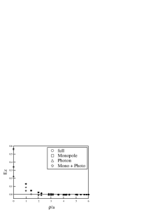
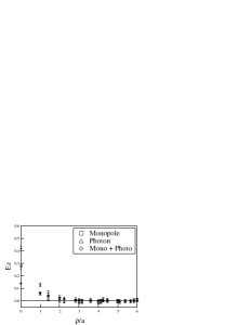
In Fig. 17, we show the result with the $3\times 3$ Wilson loop at $\beta=0.99$. Here we have used $N_{\rm conf}=1000$ configurations. These profiles are measured just on the mid-point of the Wilson loop. In Fig. 18, we also show the same electric field profiles as in Fig. 17, focussing on the region around $E_{z}\sim 0$. The important findings here are the following. The full U(1) profile is given by the sum of the photon and monopole parts, which means that Eq. (33) is satisfied. The monopole part of $E_{z}$ becomes negative beyond a certain critical radius $\rho_{c}$ (in this case $\rho_{c}/a\sim 1.5$), indicating the appearance of the solenoidal electric field, which cancels the Coulomb electric field from the photon Wilson loop at $\rho>\rho_{c}$. The corresponding schematic picture is shown in Fig. 19. There is no correlation between the photon Wilson loop and monopole current and only the monopole part is responsible for the monopole current profile. This is consistent with the fact that the solenoidal electric field is from the monopole Wilson loop (dual Ampère law). Hence, we can conclude that the U(1) flux tube has the same composite structure as the classical flux-tube solution of the DGL theory [26]. This result further supports the dual superconducting confinement mechanism (dual Meissner effect) in U(1) LGT. The behavior of the profiles from $W_{\mathit{Ph}}$ and $W_{\mathit{Mo}}$ is completely consistent with that of the static potential [27].

We find that the peak of the electric field is $E_{z}(0)=0.57$, which is larger than that in Fig. 10, $E_{z}(0)=0.38$, obtained by using the PLCF with $r/a=3$. This difference exhibits the effect of the finite temporal extension $t$ of the Wilson loop; the spatial part of the Wilson loop provides an additional Coulombic electric field. In fact, as increasing $t$, we can observe that the profile approaches to the result from the PLCF, although it becomes difficult to find a clear signal to check such a behavior without the Hodge decomposition method of the Wilson loop as shown in Figs. 20 and 21.

Figure 17: Profiles of the electric field (left) and the monopole current (right) from correlators with U(1) Wilson loop ($3\times 3$) and its photon and monopole parts.

Figure 18: The same plots as in Fig. 17 with the $E_{z}$ axis rescaled. The profile directly from the full U(1) Wilson loop is omitted.

Figure 19: The composite structure of the U(1) flux tube

Figure 20: The same plot as in Fig. 17 with W(3,5). The profiles from the full U(1) Wilson loop are omitted since they are too noisy.

Figure 21: The same plot as in Fig. 17 with W(3,7). The profiles from the full U(1) Wilson loop are omitted.

References

- [1] M. Lüscher, K. Symanzik, and P. Weisz, Nucl. Phys. B173, 365 (1980).
- [2] M. Lüscher, G. Münster, and P. Weisz, Nucl. Phys. B180, 1 (1981).
- [3] M. Caselle, R. Fiore, F. Gliozzi, M. Hasenbusch, and P. Provero, Nucl. Phys. B486, 245 (1997), hep-lat/9609041.
- [4] M. Caselle, M. Panero, and P. Provero, JHEP 06, 061 (2002), hep-lat/0205008.
- [5] M. Caselle, M. Hasenbusch, and M. Panero, JHEP 01, 057 (2003), hep-lat/0211012.
- [6] P. Majumdar, Nucl. Phys. B664, 213 (2003), hep-lat/0211038.
- [7] S. Kratochvila and Ph. de Forcrand, Observing string breaking with Wilson loops, hep-lat/0306011.
- [8] G. S. Bali, K. Schilling, and C. Schlichter, Phys. Rev. D51, 5165 (1995), hep-lat/9409005.
- [9] M. Lüscher and P. Weisz, JHEP 07, 049 (2002), hep-lat/0207003.
- [10] K. J. Juge, J. Kuti, and C. Morningstar, Phys. Rev. Lett. 90, 161601 (2003), hep-lat/0207004.
- [11] G. Arnold, T. Lippert, K. Schilling, and T. Neuhaus, Nucl. Phys. B (Proc. Suppl.) 94, 651 (2001), hep-lat/0011058.
- [12] T. A. DeGrand and D. Toussaint, Phys. Rev. D22, 2478 (1980).
- [13] T. Banks, R. Myerson, and J. Kogut, Nucl. Phys. B129, 493 (1977).
- [14] M. E. Peskin, Ann. Phys. (N.Y.) 113, 122 (1978).
- [15] V. Singh, R. W. Haymaker, and D. A. Browne, Phys. Rev. D47, 1715 (1993), hep-lat/9206019.
- [16] M. Zach, M. Faber, W. Kainz, and P. Skala, Phys. Lett. B358, 325 (1995), hep-lat/9508017.
- [17] M. Lüscher and P. Weisz, JHEP 09, 010 (2001), hep-lat/0108014.
- [18] G. Parisi, R. Petronzio, and F. Rapuano, Phys. Lett. B128, 418 (1983).
- [19] P. Majumdar, Y. Koma, and M. Koma, Nucl. Phys. B677, 273 (2004), hep-lat/0309003; in Proceedings of the 21st International Symposium on Lattice Field Theory (Lattice2003), Tsukuba, Japan, 2003, hep-lat/0309038.
- [20] Y. Koma, M. Koma, and P. Majumdar, in Proceedings of Lattice2003, hep-lat/0309056.
- [21] S. Cheluvaraja, R.W. Haymaker, and T. Matsuki, Nucl. Phys. B (Proc. Suppl.) 119, 718 (2003), hep-lat/0210016.
- [22] R. Sommer, Nucl. Phys. B411, 839 (1994), hep-lat/9310022.
- [23] P. Weisz, Nucl. Phys. B (Proc. Suppl.) 47, 71 (1996), hep-lat/9511017.
- [24] Y. Koma and H. Toki, Phys. Rev. D62, 054027 (2000), hep-ph/0004177.
- [25] Y. Koma, M. Koma, E. M. Ilgenfritz, and T. Suzuki, Phys. Rev. D (2003) in press, hep-lat/0308008.
- [26] Y. Koma, M. Koma, E.-M. Ilgenfritz, T. Suzuki, and M. I. Polikarpov, Phys. Rev. D (2003) in press, hep-lat/0302006.
- [27] J. D. Stack and R. J. Wensley, Phys. Rev. Lett. 72, 21 (1994), hep-lat/9308021.