Non-Perturbative Renormalization and the Fermilab Action

Abstract

We discuss the application of the regularization independent (RI) scheme of Rome/Southampton to determine the normalization of heavy quark operators non-perturbatively using the Fermilab action.

1 Introduction

Heavy meson hadronic matrix elements play an essential role in determining many of the parameters of the Standard Model, such as the CKM matrix elements. Theoretically, lattice gauge theory provides a means of computing these hadronic matrix elements with better control of systematic errors [1]. The heavy quark methods that have been successfully used on the lattice are: Sheikholeslami-Wohlert (SW) action, nonrelativistic QCD, heavy quark effective theory (HQET) and Fermilab action. Here we focus on the Fermilab action because it may best control the systematic errors associated with the large quark mass.

Renormalization of lattice operators is necessary in order to obtain physical results from numerical simulations. Non-perturbative renormalization (NPR) methods are attractive since they avoid possibly large errors associated with lattice perturbation theory. This is especially important when domain wall fermions are used for the light quarks. Among various NPR methods, we decide to focus on RI/MOM scheme NPR [2], because of the promising results [3] reported by the RBC collaboration. We will use NPR to represent the RI/MOM scheme NPR method in the rest of this paper.

Our goal is to adopt the RI/MOM scheme and to extend its application to heavy quarks. In particular we will show how to generalize the usual NPR “window restriction” : $\Lambda_{QCD}^{2}<<-p^{2}<<1/a^{2}$ to the kinematic region required by the Fermilab approach to heavy quarks.

2 Generalizing RI NPR to heavy quarks

We need to find a new renormalization region, which meets three requirements: i) It permits evaluation in continuum perturbation theory. Thus, it should involve non-exception external momenta, giving no infrared singularities as light quark and gluon masses are set to zero. ii) The Fermilab method remains valid, i.e. the region is not too far from the heavy quark mass pole. iii) It can be studied using a Euclidean, lattice Green’s function.

Let’s take a look at a typical Feynman diagram with a one loop QCD correction integral, for example, that shown in Figure 1, with the integral

$$\int\frac{d^{4}q}{(2\pi)^{4}}\frac{1}{q^{2}}\frac{i({\ooalign{\hfil/\hfil\crcr$p_{1}$}}-{\ooalign{\hfil/\hfil\crcr$q$}}+m)}{(p_{1}-q)^{2}-m^{2}}\frac{i({\ooalign{\hfil/\hfil\crcr$p_{2}$}}-{\ooalign{\hfil/\hfil\crcr$q$}}+m)}{(p_{2}-q)^{2}-m^{2}}.$$ (9)

Here q is the internal gluon momentum and $p_{i}$ is the net external quark momentum flowing into $i^{th}$ internal quark line within the loop.

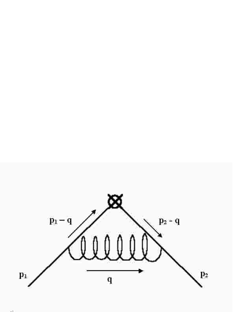
Figure 1: Example of a Feynman diagram in weak interaction effective field theory.

The denominator of the $i^{th}$ quark line, with Minkowski external momenta but Euclidean loop momentum is $(\vec{p_{i}}-\vec{q})^{2}-p_{i,0}^{2}+q_{0}^{2}+m^{2}-2ip_{i,0}\cdot q_{0}$. Since $q_{0}$ may be small, it doesn’t guarantee that we can avoid the pole on the $p_{0}$ axis during integration. Therefore, additional conditions have to be set to avoid singularities and permit the use of continuum perturbation theory. Specifically, we require that the absolute value of each denominator be much larger than $\Lambda_{QCD}^{2}$.

Let’s first check our formalism with a massless quark. We find that $-p^{2}=\mu^{2}>>\Lambda_{QCD}^{2}$, which is consistent with the the original NPR method for light quarks.

How about heavy quarks? We propose: $m^{2}-p_{0}^{2}=\mu^{2}>>\Lambda_{QCD}^{2}$. In order to keep Fermilab discretization errors under control, we have to constrain the above quantity to be much smaller than $1/a^{2}$ as well so that the heavy quark lines remain nearly on-shell. Therefore, our “window” of renormalization is $\Lambda_{QCD}^{2}<<m^{2}-p^{2}<<1/a^{2}$.

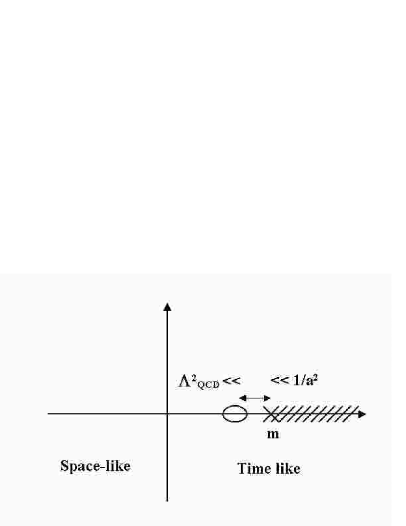
Figure 2: The complex-$p^{2}=p_{0}^{2}-{\vec{p}}^{2}$ plane.

Figure 2 is a plot in complex $p^{2}$ plane. Our choice of renormalization points are located within the small region circled. The distance from this circled region to the mass pole has to be much smaller than $\frac{1}{a^{2}}$ and much larger $\Lambda_{QCD}^{2}$ for perturbation theory to be valid. This is what I mean by “slightly off-shell condition” in the rest of the paper.

Note that the region we choose is time-like, while the usual NPR’s choice is space-like. Why do we pick a time-like point, instead of a space-like point? The constraint comes from the Fermilab action, which is an on-shell O(a) improvement. If we choose a deep, space-like point, the well-behaved properties of Fermilab action would no longer be valid.

3 Off-shell Fermilab action

Recall “heavy quark” means the product of $m$ and lattice spacing $a$ may be larger than or equal to 1. Under this circumstance, it’s natural to expect an improved action to break the time-space symmetry. Here is the original Fermilab action [4]:

$$S = \sum_{n}\bar{\psi_{n}}\psi_{n}{}$$ (10)

$$- \hskip-10.84006pt\kappa_{t}\sum_{n}[\bar{\psi_{n}}(1-\gamma_{0})\textsl{U}_{n,0}\psi_{n+\hat{0}}+\bar{\psi}_{n+\hat{0}}(1+\gamma_{0})\textsl{U}_{n,0}^{\dagger}\psi_{n}]$$

$$- \hskip-10.84006pt\kappa_{s}\sum_{n,i}[\bar{\psi}_{n}(r_{s}-\gamma_{i})\textsl{U}_{n,i}+\bar{\psi}_{n+\hat{i}}(r_{s}+\gamma_{i})\textsl{U}_{n,i}^{\dagger}\psi_{n}]$$

$$+ \hskip-10.84006pt\frac{i}{2}c_{B}\kappa_{s}\sum_{n;i,j,k}\varepsilon_{ijk}\bar{\psi}_{n}\sigma_{ij}B_{n;k}\psi_{n}$$

$$+ \hskip-10.84006ptic_{E}\kappa_{s}\sum_{n;i}\bar{\psi}_{n}\sigma_{0i}E_{n;i}\psi_{n}$$

Note that those coefficients are the functions of $ma$, and are expected to remain finite for both small and large $ma$.

What happens when we go slightly off-shell? If the external quark masses differ from the physical ones by a small amount $\delta m$, with $a\delta m\ll 1$ then the resulting errors will be no larger than the other discretization errors in the Fermilab approach.

However, when we go off-shell, we have to include more terms to make the O(a) improvement complete. (Why? because contact terms and new non-gauge-invariant operators can appear.) First, we have to add O(a) off-shell improvement terms in the action. Fortunately, those terms which need to be added in the action can be compensated by improving the quark fields [5]. Therefore, the action itself remains the same, including the well-behaved coefficients.

The improved quark fields will look similar to those in ref [5], but with broken space-time symmetry. Likewise for the composite operators. The broken symmetry gives us at least double the number coefficients to be determined non-perturbatively, compared with the light quark cases. We are still exploring how these coefficients may be determined in a more efficient way.

4 Imposing RI NPR on the lattice

To respect the “slightly off-shell condition”, we need to change the time-component Fourier transformation to Laplace transformation. Take the operator $O_{\Gamma}(x)=\bar{\psi}(x)\Gamma\psi(x)$ as an example, for a general Dirac matrix $\Gamma$. The non-amputated Green’s function in momentum space is:

$$G_{O}(pa)=\langle S_{\{U\}}(p\mid 0)\;\Gamma\;\gamma_{5}{S}_{\{U\}}^{\dagger}(p\mid 0)\gamma_{5}\rangle|_{\{U\}}$$ (11)

where $S_{i}(p\mid y)=\int d^{3}x\int dx_{0}S_{i}(x\mid y)e^{+ip\cdot x}e^{p_{0}x_{0}}$.

We calculate the amputated Green’s function and apply the projector onto $\hat{P}_{O}$ to define:

$$\Gamma_{O}(pa)=\frac{1}{12}Tr[S(pa)^{-1}G_{O}(pa)S(pa)^{-1}\hat{P}_{O}],$$ (12)

where the S(pa) is the gauge-averaged propagator. Following the usual NPR procedure, we apply the renormalization condition:

$$\langle p|O_{\Gamma}^{NPR}|p\rangle\mid_{m^{2}-p^{2}={\mu}^{2}}\;=\langle p|O_{\Gamma}|p\rangle_{0},$$ (13)

where $\langle...\rangle_{0}$ represents tree-level value. Thus, imposing $Z_{O}Z_{\psi}^{-1}\Gamma_{O}|_{m^{2}-p^{2}={\mu}^{2}}\;=1$ will determine the renormalization factor $Z_{O}(\mu a,g(a))$.

5 Matching to the $\overline{MS}$ scheme

Our lattice NPR calculations are done in the RI renormalization scheme. We need continuum RI renormalization calculations to match to physical values given in the continuum $\overline{MS}$ scheme. The previous matching calculations done at $-p^{2}=\mu^{2}$, while taking $m\rightarrow 0$ must be extended to our new scheme.

Let’s take a look at the simplest example: the calculation of $Z_{q}$ and $Z_{m}$. Our new renormalization conditions become:

$$\frac{1}{48}Z_{q}Tr[\gamma_{\mu}\frac{\partial({\ooalign{\hfil/\hfil\crcr$p$}}\bar{\Sigma}_{1}(p))}{\partial p_{\mu}}]_{m^{2}-p^{2}=\mu^{2}}=1$$ (16)

$$\frac{1}{12}Z_{q}Z_{m}Tr[\bar{\Sigma}_{2}(p)]_{m^{2}-p^{2}=\mu^{2}}=1$$ (17)

where $iS^{-1}(p)=Z_{q}[{\ooalign{\hfil/\hfil\crcr$p$}}\bar{\Sigma}_{1}(p)-Z_{m}m\bar{\Sigma}_{2}(p)]$.

The calculations are done in the dimensional regularization scheme, where D is 4-2$\epsilon$. Here are the matching factors for $Z_{m}$ and $Z_{q}$ in the RI and $\overline{MS}$ schemes:

$$\frac{Z_{m}^{RI}}{Z_{m}^{\overline{MS}}}\hskip-7.22743pt = 1-\frac{\alpha_{s}}{4\pi}\frac{N_{c}^{2}-1}{2N_{c}}\{\frac{8+3\xi}{2}-3\xi\frac{m^{2}}{m^{2}-\mu^{2}}$$ (18)

$$- \hskip-10.84006pt[(3+\xi)\frac{m^{2}}{m^{2}-\mu^{2}}-3\xi\frac{m^{4}}{(m^{2}-\mu^{2})^{2}}]ln\frac{m^{2}}{\mu^{2}}$$

$$+ \hskip-10.84006ptln\frac{\mu^{\prime}\;{}^{2}}{\mu^{2}}(3+2\xi)\}+O(\alpha_{s}^{2})$$

$$\frac{Z_{q}^{RI}}{Z_{q}^{\overline{MS}}}\hskip-7.22743pt = 1-\frac{\alpha_{s}}{4\pi}\frac{N_{c}^{2}-1}{2N_{c}}\xi(\frac{1}{2}+3\frac{m^{2}}{m^{2}-\mu^{2}}{}$$

$$- 3 \hskip-10.84006pt\frac{m^{4}}{(m^{2}-\mu^{2})^{2}}ln\frac{m^{2}}{\mu^{2}}-ln\frac{\mu^{\prime}\;{}^{2}}{\mu^{2}})+O(\alpha_{s}^{2}),$$ (19)

where $\mu^{\prime}$ is defined as $g_{0}=Z_{g}g\mu^{\prime}\;{}^{\epsilon}$.

6 Conclusion

In this paper, we present a first NPR renormalization proposal for relativistic heavy quarks. We propose a new renormalization point: $\Lambda_{QCD}^{2}<<m^{2}-p^{2}<<1/a^{2}$, in a slightly off-shell region. We must add off-shell improvement terms and determine the corresponding coefficients as well as evaluating Laplace transformations in the time.

The author would like to thank each member of the RBC collaboration for their assistance. Special thanks go to N. H. Christ for inspiration and constant discussions on various topics.

References

- [1] S. M. Ryan, Nucl.Phys.Proc.Suppl. 106, 86 (2002), hep-lat/0111010; N. Yamada , hep-lat/0210035.
- [2] G. Martinelli et al., Nucl.Phys. B445, 81 (1995), hep-lat/9411010; V. Gimenez et al., Nucl.Phys. B531, 429 (1998), hep-lat/9806006; A. Doninir et al., Eur.Phys.J. C10, 121 (1999), hep-lat/9902030.
- [3] T. Blum et al. (RBC), (2001), hep-lat/0110075; T. Blum et al. (RBC), Phys.Rev. D66, 014504 (2002), hep-lat/0102005.
- [4] A. X. El-Khadra et al. , Phys.Rev. D55, 3933 (1999), hep-lat/9604004.
- [5] G. Martinelli et al., Nucl.Phys. B611, 311 (2001), hep-lat/0106003.