Lattice regularized chiral perturbation theory

Abstract

Chiral perturbation theory can be defined and regularized on a spacetime lattice. A few motivations are discussed here, and an explicit lattice Lagrangian is reviewed. A particular aspect of the connection between lattice chiral perturbation theory and lattice QCD is explored through a study of the Wess-Zumino-Witten term.

1 MOTIVATIONS

The spacetime lattice is a regularization technique for quantum field theories. Interest in the lattice regularization of chiral perturbation theory (ChPT) has arisen in a number of different contexts.

1.1 Discretization effects for lattice QCD

To account for the effects of nonzero lattice spacing, $a$, in lattice QCD simulations, work has been done to include explicit $a$-dependences into the effective field theory, ChPT. Since $1/a$ in lattice QCD simulations is typically larger than the chiral scale $\Lambda_{\chi}\sim 1$ GeV, it is common to include these $a$-dependences by adding extra “irrelevant” operators to ChPT [1, 2, 3]. Calculations are then performed in the continuum, using dimensional regularization or some other continuum regularization method, and results contain both $a$-dependent terms and $\mu$-dependent terms where $\mu$ is the regularization scale. As usual, physical observables will be independent of $\mu$ in a regime where ChPT is applicable and has acceptable convergence properties.

Alternatively, one might prefer to define lattice ChPT as an effective theory that exists directly in the same discrete spacetime where lattice QCD resides[4, 5, 6]. With this approach the lattice itself regulates the theory, playing the roles that were assigned to both $\mu$ and $a$ in the continuum method discussed above. This type of lattice ChPT has no divergences for nonzero $a$ and it has no need for a continuum regulator. With small lattice spacings, i.e. $1/a\gg\Lambda_{\chi}$, physical observables will be essentially independent of the regularization scheme and scale, so the results will reproduce those obtainable from the continuum theory of the previous paragraph (up to negligible differences that vanish exactly as $a\to 0$).

On coarse lattices, perhaps $1/a\sim\Lambda_{\chi}$, it is important to determine whether the scheme dependence really is acceptably negligible before relying on a particular regularization scheme. Explicit lattice ChPT studies of physical observables over a range of lattice spacings can help to quantify how small the lattice spacing must be to ensure that this type of scheme dependence is indeed negligible.

1.2 Convergence and power divergences

Lattice regularized ChPT is also of interest independently of its connection to lattice QCD. There has recently been renewed interest in cut-off type regularization schemes for ChPT[7, 8, 9], and in this context lattice regularized ChPT might be viewed as yet another way to implement a cut-off.

Ref. [7] contains some studies of the convergence of ChPT by using a particular momentum cut-off scheme, referred to as long-distance regularization, and studying the cut-off dependences order by order in the chiral expansion. Although each observable needs to be essentially independent of regularization scheme, the convergence of ChPT is typically defined in a scheme-dependent fashion by comparing the relative sizes of the contributions to some observable at each chiral order. Like most regularization schemes (but unlike dimensional regularization) cut-off schemes have power divergent loop integrals, and variation of the cut-off can significantly change the size of loop contributions relative to counterterms. Such studies provide insight into the convergence of ChPT and into the effect of having to truncate ChPT at some fixed chiral order.

The Adelaide group has discussed scheme dependence and convergence for a collection of “finite range regulators”[8], similar to the long-distance regularization scheme mentioned above, and they have made extensive studies of their method in the context of practical extrapolations for lattice QCD data.

Lattice regularized ChPT is also a method for invoking a cut-off, with its own specific features. A potential disadvantage of the lattice method is that the continuous rotational symmetry is reduced to a hypercubic rotational symmetry, though this only becomes significant at the very short distance scale set by the lattice spacing. An advantage of the lattice method is that the lattice spacing appears directly in the Lagrangian, in contrast to schemes where the cut-off is inserted by hand into each loop integration. Therefore every calculation with the lattice method automatically preserves all of the Lagrangian’s symmetries (like chiral symmetry and gauge invariance) whereas the users of other cut-off methods must be careful to ensure that implementation of the cut-off preserves the desired symmetries during the calculation of each loop integral.

1.3 Nonperturbative issues

A particularly valuable feature of lattice regularization is that it does not rely on perturbation theory. Lattice QCD takes advantage of this, and a multi-nucleon effective field theory might also find lattice regularization to be a useful tool.[10] In the present work, we will restrict ourselves to ChPT in the presence of at most a single baryon.

2 MESON SECTOR

Chiral perturbation theory is an expansion in inverse powers of $\Lambda_{\chi}\sim 4\pi{F_{\pi}}\sim 4\pi{F_{K}}\sim 1$ GeV. In Euclidean spacetime, the familiar chiral Lagrangian[11] for pseudoscalar mesons is

$${\cal L}_{\rm M} \!=\! {\cal L}_{\rm M}^{(2)}+{\cal L}_{\rm M}^{(4)}+{\cal L}_{\rm M}^{(6)}+\ldots,$$ (1)

$${\cal L}_{\rm M}^{(2)} \!=\! \frac{F^{2}}{4}{\rm Tr}(\sum_{\mu}\nabla_{\mu}{U}^{\dagger}\nabla_{\mu}{U}-\chi^{\dagger}{U}-\chi{U}^{\dagger}),$$ (2)

$${\cal L}_{\rm M}^{(4)} \!=\! -L_{1}\left(\sum_{\mu}{\rm Tr}(\nabla_{\mu}{U}^{\dagger}\nabla_{\mu}{U})\right)^{2}$$ (3)

$$-L_{2}\sum_{\mu,\nu}{\rm Tr}(\nabla_{\mu}{U}^{\dagger}\nabla_{\nu}{U}){\rm Tr}(\nabla_{\mu}{U}^{\dagger}\nabla_{\nu}{U})$$

$$-L_{3}\sum_{\mu,\nu}{\rm Tr}(\nabla_{\mu}{U}^{\dagger}\nabla_{\mu}{U}\nabla_{\nu}{U}^{\dagger}\nabla_{\nu}{U})$$

$$+L_{4}\sum_{\mu}{\rm Tr}(\nabla_{\mu}{U}^{\dagger}\nabla_{\mu}{U}\}{\rm Tr}\{\chi^{\dagger}{U}+\chi{U}^{\dagger})$$

$$+L_{5}\sum_{\mu}{\rm Tr}(\nabla_{\mu}{U}^{\dagger}\nabla_{\mu}{U}(\chi^{\dagger}{U}+U^{\dagger}\chi))$$

$$-L_{6}\left({\rm Tr}(\chi^{\dagger}{U}+\chi{U}^{\dagger})\right)^{2}$$

$$-L_{7}\left({\rm Tr}(\chi^{\dagger}{U}-\chi{U}^{\dagger})\right)^{2}$$

$$-L_{8}{\rm Tr}(\chi^{\dagger}{U}\chi^{\dagger}{U}+\chi{U}^{\dagger}\chi{U}^{\dagger})$$

$$+iL_{9}\sum_{\mu,\nu}{\rm Tr}(F^{R}_{\mu\nu}\nabla_{\mu}{U}\nabla_{\nu}{U}^{\dagger}$$

$$+F^{L}_{\mu\nu}\nabla_{\mu}{U}^{\dagger}\nabla_{\nu}{U})$$

$$-L_{10}\sum_{\mu,\nu}{\rm Tr}(U^{\dagger}{F}^{R}_{\mu\nu}UF^{L}_{\mu\nu}),$$

where the fields are

$$U(x) = \exp\left[\frac{-i\lambda^{a}\pi^{a}(x)}{F}\right],$$ (4)

$$\chi = 2B\left(\begin{array}[]{ccc}m_{u}&0&0\\ 0&m_{d}&0\\ 0&0&m_{s}\end{array}\right)+\ldots,$$ (8)

$$L_{\mu}(x) = \exp[-ia\ell_{\mu}(x)],$$ (9)

$$R_{\mu}(x) = \exp[-iar_{\mu}(x)].$$ (10)

This Lagrangian is invariant under a local chiral transformation,

$$U(x) \to g(x)U(x)h(x),$$ (11)

$$R_{\mu}(x) \to g(x)R_{\mu}(x)g^{\dagger}(x+a_{\mu}),$$ (12)

$$L_{\mu}(x) \to h^{\dagger}(x)L_{\mu}(x)h(x+a_{\mu}),$$ (13)

if the covariant derivatives are defined appropriately. To avoid extra (unphysical) states in the dispersion relation, a nearest-neighbour derivative will be used in ${\cal L}_{\rm M}^{(2)}$,

$$a\nabla_{\mu}^{(+)}U(x)=R_{\mu}(x)U(x+a_{\mu})L_{\mu}^{\dagger}(x)-U(x).$$ (14)

Use of this derivative at higher chiral orders would not preserve parity, so a symmetric derivative is used everywhere except ${\cal L}_{\rm M}^{(2)}$,

$$2a\nabla_{\mu}^{(\pm)}U(x) \!\!\!\!=\!\!\!\! R_{\mu}(x)U(x+a_{\mu})L_{\mu}^{\dagger}(x)$$

$$\!\!\!\!-\!\!\!\! R_{\mu}^{\dagger}(x-a_{\mu})U(x-a_{\mu})L_{\mu}(x-a_{\mu}).$$

It should be emphasized that the lattice ChPT Lagrangian obtained by putting these lattice derivatives into Eqs. (1-3) is not the most general one that could be written on a hypercubic lattice; it is merely one example of a ChPT Lagrangian that has the correct continuum limit. Similarly, there is an entire family of lattice QCD Lagrangians that approach the unique continuum QCD as $a\to 0$. As discussed in section 1, extra irrelevant operators that contain explicit powers of $a$ can be added to the ChPT Lagrangian of Eqs. (1-3) and a particular choice for the set of associated coefficients would correspond to a particular choice for the underlying lattice QCD Lagrangian. Since our intent is mainly to study regularization issues, we will arbitrarily set all of these extra coefficients to zero for simplicity.

Our full action contains the usual Lagrangian term plus a less familiar term which arises from the integration measure[12],

$$S_{\rm M} = a^{4}\sum_{x}{\cal L}_{\rm M}(x)$$ (16)

$$-\frac{1}{2}\sum_{x}{\rm Tr}\ln\left[\frac{2(1-\cos\Phi(x))}{\Phi^{2}(x)}\right]$$

where $\Phi(x)=\frac{2}{F}\sum_{a=1}^{8}t^{a}\pi^{a}(x)$ with $t^{a}_{bc}=-if_{abc}$.

For a sample calculation, consider the meson masses. Neglecting isospin violation ($m_{l}\equiv m_{u}=m_{d}$), the lowest order pion, kaon and eta two point functions are

$$\Gamma_{MM}=-\left[x_{M}^{2}+\frac{4}{a^{2}}\sum_{\mu}\sin^{2}\left(\frac{aq_{\mu}}{2}\right)\right]$$ (17)

where $M=\pi$, $K$ or $\eta$ and

$$x_{\pi} = \sqrt{2Bm_{l}},$$ (18)

$$x_{K} = \sqrt{B(m_{l}+m_{s})},$$ (19)

$$x_{\eta} = \sqrt{\frac{2}{3}B(m_{l}+2m_{s})}.$$ (20)

The meson masses are therefore

$$m_{M}=\frac{2}{a}{\rm arcsinh}\left(\frac{ax_{M}}{2}\right).$$ (21)

Notice the existence of a Gell-Mann–Okubo relation

$$3{\rm sinh}^{2}\left(\frac{am_{\eta}}{2}\right)=4{\rm sinh}^{2}\left(\frac{am_{K}}{2}\right)-{\rm sinh}^{2}\left(\frac{am_{\pi}}{2}\right)$$

which reproduces the conventional relation as $a\rightarrow 0$. The next-to-leading order expressions include one-loop diagrams and ${\cal L}_{\rm M}^{(4)}$ tree-level pieces. Loop momentum integration is from $-\pi/a$ to $+\pi/a$, representing the complete range of momenta available in the lattice theory. The results have the form

$$\Gamma_{MM} \!\!\!\!=\!\!\!\! \frac{-1}{Z_{M}^{(+)}Z_{M}^{(\pm)}}\left[X_{M}^{2}+\frac{4Z_{M}^{(\pm)}}{a^{2}}\sum_{\mu}\sin^{2}\left(\frac{aq_{\mu}}{2}\right)\right.$$ (23)

$$\left.+\left(\frac{1-Z_{M}^{(\pm)}}{a^{2}}\right)\sum_{\mu}\sin^{2}\left(aq_{\mu}\right)\right],$$

where $X_{M}$, $Z_{M}^{(+)}$ and $Z_{M}^{(\pm)}$ contain five Lagrangian parameters, $L_{4}$, $L_{5}$, $L_{6}$, $L_{7}$, $L_{8}$, and a single integral,

$$W_{4}(\epsilon)\equiv\int_{0}^{\infty}{\rm d}x\,I_{0}^{4}(x)\exp\left[-x\left(4+\frac{\epsilon}{2}\right)\right]$$ (24)

where $I_{0}(x)$ is a Bessel function. For example, the kaon mass is

$$m_{K}=\frac{2}{a}{\rm arcsinh}\left(\frac{aX_{K}}{2}\right)$$ (25)

where

$$X_{K}^{2} \!\!\!=\!\!\! x_{K}^{2}-\frac{8}{F^{2}}x_{K}^{2}(x_{\pi}^{2}+2x_{K}^{2})(L_{4}-2L_{6})$$ (26)

$$-\frac{8}{F^{2}}x_{K}^{4}(L_{5}-2L_{8})+\frac{7x_{K}^{2}}{24a^{2}F^{2}}$$

$$+\frac{x_{K}^{2}}{6a^{2}F^{2}}W_{4}(a^{2}x_{\eta}^{2})-\frac{3x_{\pi}^{2}x_{K}^{2}}{64F^{2}}W_{4}(a^{2}x_{\pi}^{2})$$

$$-\frac{3x_{K}^{4}}{32F^{2}}W_{4}(a^{2}x_{K}^{2})-\frac{x_{K}^{2}x_{\eta}^{2}}{192F^{2}}W_{4}(a^{2}x_{\eta}^{2}).$$

Notice that the kaon mass vanishes in the chiral limit ($m_{l}=m_{s}=0$), consistent with the fact that the theory does indeed have exact chiral symmetry even for $a\neq 0$.

As $a\to 0$, loop integrals diverge but the infinities can be absorbed into renormalized parameters. The meson masses and the scale dependences of the counterterms are in analytic agreement with dimensional regularization. For example, defining $\Delta L_{i}\equiv L_{i}^{r}(1/a_{2})-L_{i}^{r}(1/a_{1})$, one finds

$$\Delta L_{4}-2\Delta L_{6} = -\frac{1}{36(4\pi)^{2}}\ln\left(\frac{a_{2}}{a_{1}}\right),$$ (27)

$$\Delta L_{5}-2\Delta L_{8} = \frac{1}{6(4\pi)^{2}}\ln\left(\frac{a_{2}}{a_{1}}\right),$$ (28)

$$3\Delta L_{7}+\Delta L_{8} = \frac{5}{48(4\pi)^{2}}\ln\left(\frac{a_{2}}{a_{1}}\right),$$ (29)

for sufficiently small lattice spacings $a_{1}$ and $a_{2}$. These are precisely the same logarithms and numerical coefficients that appear in dimensional regularization[11]. Power divergences do arise in lattice regularized loop integrals, and they always get absorbed into Lagrangian parameters during renormalization.

3 HEAVY BARYON SECTOR

Heavy baryon chiral perturbation theory (HBChPT) is an expansion in the inverse baryon mass as well as the inverse chiral scale, $\Lambda_{\chi}$. The heavy octet baryon field is

$$B_{v}(x)=\exp(im_{\rm HB}v\cdot{x})\frac{1}{2}(1+v\!\!\!/)B(x),$$ (30)

where $m_{\rm HB}$ is chosen near the physical baryon mass.

The first few orders in the double expansion of Euclidean HBChPT are

$${\mathcal{L}}_{\rm MB} = {\mathcal{L}}_{\rm MB}^{(0)}+{\mathcal{L}}_{\rm MB}^{(1)}+{\mathcal{L}}_{\rm MB}^{(2)}+{\mathcal{L}}_{\rm MB}^{(3)}+\ldots,$$ (31)

$${\mathcal{L}}_{\rm MB}^{(0)} = (m_{0}-m_{\rm HB}){\rm Tr}\left(\bar{B}_{v}B_{v}\right),$$ (32)

$${\mathcal{L}}_{\rm MB}^{(1)} = \sum_{\mu}{\rm Tr}\bar{B}_{v}(v_{\mu}D_{\mu}B_{v}+{\mathcal{D}}S_{\mu}\{u_{\mu},B_{v}\}$$ (33)

$$+{\mathcal{F}}S_{\mu}[u_{\mu},B_{v}]),$$

$${\mathcal{L}}_{\rm MB}^{(2)} = \frac{1}{2m_{0}}{\rm Tr}\bar{B}_{v}(v\cdot{D}v\cdot{D}-D^{2})B_{v}$$ (34)

$$-{\rm Tr}\bar{B}_{v}\left(b_{\mathcal{D}}\{\chi_{+},B_{v}\}+b_{\mathcal{F}}[\chi_{+},B_{v}]\right)$$

$$-b_{0}{\rm Tr}\left(\bar{B}_{v}B_{v}\right){\rm Tr}\left(\chi_{+}\right)$$

$$+\frac{i}{4m_{0}}\sum_{\mu,\nu}{\rm Tr}\bar{B}_{v}[S_{\mu},S_{\nu}]\times$$

$$(\mu_{D}\{\xi F_{\mu\nu}^{L}\xi^{\dagger}+\xi^{\dagger}F_{\mu\nu}^{R}\xi,B_{v}\}$$

$$+\mu_{F}[\xi F_{\mu\nu}^{L}\xi^{\dagger}+\xi^{\dagger}F_{\mu\nu}^{R}\xi,B_{v}])+\ldots$$

where $\mathcal{D}$ and $\mathcal{F}$ are the axial couplings, and $S_{\mu}=\frac{i}{2}\gamma_{5}\sum_{\nu}\sigma_{\mu\nu}v_{\nu}$.
The mesons are contained within

$$U = \xi^{2},$$ (35)

$$\chi_{+} = \xi^{\dagger}\chi\xi^{\dagger}+\xi\chi^{\dagger}\xi,$$ (36)

$$u_{\mu}(x) = \frac{i}{2}\xi^{\dagger}(x)\nabla_{\mu}^{(\pm)}U(x)\xi^{\dagger}(x)$$ (37)

$$- \frac{i}{2}\xi(x)\nabla_{\mu}^{(\pm)}U^{\dagger}(x)\xi(x).$$

It is convenient to choose the velocity parameter to have only a temporal component, $v=(0,0,0,1)$, and to use a nearest-neighbour temporal derivative $D_{4}$ but a next-nearest-neighbour spatial derivative $D_{i}$, since this preserves parity without introducing unphysical states. As was discussed for the meson Lagrangian, the most general lattice HBChPT Lagrangian will contain additional terms that have explicit powers of the lattice spacing. The coefficients of these terms could be chosen by matching to a specific version of lattice QCD, but here we set them all to zero and use the remaining “minimal” lattice ChPT that still has the unique continuum limit.

To incorporate the decuplet baryons as heavy fields, we use[13]

$${\cal L}_{\rm MT}^{(1)} = -\sum_{\mu\nu}\sum_{ijk}\bigg{(}\bar{T}_{v\mu}^{ijk}v_{\nu}D_{\nu}T_{v\mu}^{ijk}$$ (38)

$$-{\cal H}\sum_{l}\bar{T}_{v\mu}^{ijk}S_{\nu}u_{\nu}^{kl}T_{v\mu}^{ijl}\bigg{)}$$

$$-\Delta\sum_{\mu}\sum_{ijk}\bar{T}_{v\mu}^{ijk}T_{v\mu}^{ijk},$$

$${\cal L}_{\rm MBT}^{(1)} = \frac{\cal C}{2}\sum_{\mu}\sum_{ijklm}\epsilon_{ijk}(\bar{T}_{v\mu}^{klm}u_{\mu}^{mj}B_{v}^{li}$$ (39)

$$+\bar{B}_{v}^{il}u_{\mu}^{jm}T_{\mu}^{klm}).$$

The resulting spin-3/2 propagator is

$$\frac{-P^{3/2}_{\mu\nu}}{\Gamma_{TT}}=\frac{ia(\delta_{\mu\nu}-v_{\mu}v_{\nu}+\frac{4}{3}S_{\mu}S_{\nu})}{\sin(ap_{4})-i[a\Delta+2\sin^{2}(ap_{4}/2)]}.$$ (40)

Calculations can now be done in a straightforward manner, just as was discussed for the meson sector, and some specific calculations can be found in Ref. [6]. Loop integrals generally contain power divergences as $a\to 0$ — for an $O(p^{3})$ calculation they can be cubic, quadratic and linear — but these can always be absorbed into Lagrangian parameters. Gauge invariance is also automatically preserved, and an explicit calculation is discussed in detail in Ref. [6].

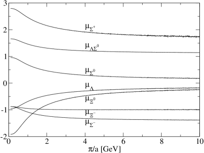
Figure 1: Octet baryon magnetic moments from ChPT parameters that reproduce the experimental values for $\mu_{p}$ and $\mu_{n}$ at all lattice spacings.

Figure 1 shows the results of an $O(p^{3})$ calculation of the octet baryon magnetic moments as functions of the lattice spacing. For this illustrative example, parameters were chosen such that the proton and neutron magnetic moments are equal to their experimental values at all lattice spacings. All of the remaining octet baryon magnetic moments are plotted in the figure, and Table 1 shows the numerical difference between results in the continuum and results at $a=0.1$ fm.

Two aspects of this illustrative example should be emphasized at this point. First, it is well known that $O(p^{4})$ corrections to the baryon magnetic moments can be significant[14]. Since our calculation is intended to be a simple example of discretization effects, not a high precision determination of the magnetic moments, we have not concerned ourselves with the addition of $O(p^{4})$ terms. Secondly, the lattice spacing dependences computed here are, of course, specific to the minimal version of lattice ChPT that we have employed, where a collection of coefficients has been set to zero instead of being matched to some specific lattice QCD Lagrangian.

Table 1: The numerical distinction between magnetic moments in the continuum and at $a=0.1$ fm, for a specific lattice ChPT Lagrangian.

$B$	$\mu_{B}(a=0)$	$\frac{\mu_{B}(a=0.1{\rm fm})}{\mu_{B}(a=0)}$
$\Sigma^{+}$	1.64	1.11
$\Sigma^{0}$	0.12	1.94
$\Sigma^{-}$	-1.40	0.97
$\Xi^{0}$	-0.14	2.58
$\Xi^{-}$	-0.98	1.01
$\Lambda$	-0.12	1.95
$\Lambda\Sigma^{0}$	1.11	1.05

4 WESS-ZUMINO-WITTEN SECTOR

The Wess-Zumino-Witten (WZW) effective action accounts for the physics of the chiral anomalies.[15] A lattice representation of the WZW action can be constructed by converting derivatives to finite differences, just as was done above for the non-anomalous meson and baryon sectors. However, the WZW action is special in that its continuum form can be uniquely derived — with no unknown coefficients at leading chiral order — from an underlying fermion action. In fact, Aoki has shown that the unique continuum WZW action can be derived from the lattice Wilson action.[16, 17]

Alternatively, one might be interested in defining a lattice effective action that resides in the same discrete spacetime where the underlying fermion action (Wilson, for example) resides. However, a unique lattice WZW effective action cannot be derived from the Wilson fermion action. Here, we discuss this issue by closely following the work of Refs. [16, 17] but without invoking the continuum.

Begin with massless Wilson fermions coupled to external gauge fields.

$$S^{(W)}(L,R)=$$

$$\frac{1}{2}\sum_{n,\mu}(\bar{\psi}^{L}_{n}\gamma_{\mu}L_{n,n+\mu}\psi^{L}_{n+\mu}-\bar{\psi}^{L}_{n}\gamma_{\mu}L_{n,n-\mu}\psi^{L}_{n-\mu}$$

$$+\bar{\psi}^{R}_{n}\gamma_{\mu}R_{n,n+\mu}\psi^{R}_{n+\mu}-\bar{\psi}^{R}_{n}\gamma_{\mu}R_{n,n-\mu}\psi^{R}_{n-\mu})$$

$$-\frac{r}{2}\sum_{m,n}\left(\bar{\psi}^{L}_{m}\Box_{m,n}\psi^{R}_{n}+\bar{\psi}^{R}_{m}\Box_{m,n}\psi^{L}_{n}\right).$$ (41)

Except for the chiral symmetry breaking Wilson term (proportional to $r$), this action is invariant under local chiral transformations,

$$\psi^{L}_{n} \to h_{n}\psi^{L}_{n},$$ (42)

$$\psi^{R}_{n} \to g_{n}\psi^{R}_{n},$$ (43)

$$L_{m,n} \to h_{m}L_{m,n}h^{\dagger}_{n},$$ (44)

$$R_{m,n} \to g_{m}R_{m,n}g^{\dagger}_{n},$$ (45)

where $h_{n}\in SU_{L}(N_{f})$ and $g_{n}\in SU_{R}(N_{f})$. To obtain the WZW effective action, consider the axial transformation,

$$\psi^{L}_{n} \to u_{n}^{\dagger}\psi^{L}_{n},$$ (46)

$$\psi^{R}_{n} \to u_{n}\psi^{R}_{n},$$ (47)

$$L_{m,n} \to L_{m,n}^{\prime}\equiv u^{\dagger}_{m}L_{m,n}u_{n},$$ (48)

$$R_{m,n} \to R_{m,n}^{\prime}\equiv u_{m}R_{m,n}u^{\dagger}_{n},$$ (49)

where $u_{n}^{2}=U_{n}=\exp(-i\lambda^{a}\pi^{a}_{n}/F)$. The WZW action is defined to be the difference

$$W_{WZW}=W(L^{\prime},R^{\prime})-W(L,R)$$ (50)

where, as usual,

$$Z(L,R) = \exp(-W(L,R))$$ (51)

$$= \int{\cal D}\bar{\psi}{\cal D}\psi\,\exp\left(-S^{(W)}(L,R)\right).$$

After using $W=-\ln\det D=-{\rm Tr}\ln D$, inserting a complete set of states into the trace, and performing some further algebra, one arrives at

$$W_{WZW} \!\!\!\!\!=\!\!\!\!\! \frac{N_{c}}{4}\sum_{n}\int_{0}^{1}\!\!\!d\tau\int_{-\pi}^{\pi}\frac{d^{4}k}{(2\pi)^{4}}\sum_{m=0}^{\infty}\frac{{\rm Tr}_{n}(A_{m,n})}{(-s^{2})^{m+1}}$$

where $n$ sums over all lattice sites but $m$ is just an integer index. Also,

$$A_{m,n} \!\!\!\!\!=\!\!\!\!\! s\!\!/\!\left[\left(LT\!\!\!/P^{L}\!+\!RT\!\!\!/P^{R}\!+\!P^{L}Q_{L}\!+\!P^{R}Q_{R}\right)s\!\!/\right]^{m}$$ (53)

$$\times\frac{d~{}}{d\tau}\left[P^{L}Q_{L}+P^{R}Q_{R}\right]$$

and $\tau$ is the coordinate of Witten’s extra dimension, so $u^{\tau}_{n}\in SU(N_{f})$ with $u^{0}_{n}=1$ and $u_{n}^{1}=u_{n}$. We have also defined

$$Q_{L} = -ru^{\dagger}\bigg{(}\sum_{\mu}Q^{\mu}\bigg{)}u^{\dagger},$$ (54)

$$Q_{R} = -ru\bigg{(}\sum_{\mu}Q^{\mu}\bigg{)}u,$$ (55)

$$Q_{m,n}^{\mu} = \Box_{m,n}\cos(k_{\mu})+i\partial_{m,n}\sin(k_{\mu})$$ (56)

$$-2\delta_{m,n}(1-\cos(k_{\mu})),$$

$$T_{m,n}^{\mu} = 2\partial_{m,n}\cos(k_{\mu})+i\Box_{m,n}\sin(k_{\mu}),$$ (57)

$$\partial_{m,n} = (\delta_{m+\mu,n}-\delta_{m-\mu,n})/2,$$ (58)

$$\Box_{m,n} = \delta_{m+\mu,n}+\delta_{m-\mu,n}-2\delta_{m,n},$$ (59)

and $P_{R,L}=(1\pm\gamma_{5})/2$.

In the continuum limit, $\partial_{m,n}$ and $\Box_{m,n}$ collapse to local derivatives and the summations can be performed explicitly.[17] The expression for $W_{WZW}$ reproduces the well-known anomaly. On a lattice, the summation over $m$ in Eq. (LABEL:Wwzw) does not produce a closed analytic form. We have worked through the case of 2-dimensional spacetime in some detail, and find that terms with arbitrarily many powers of $Q^{\mu}$, as defined in Eq. (56), can contribute at low chiral orders. The essential point is that “$\lim_{a\to 0}$” and “${\rm Tr}_{n}$” do not commute. Notice that Tr_n requires closed paths on the lattice.

5 SUMMARY

Lattice regularization can be applied to chiral perturbation theory. The simplest lattice ChPT Lagrangian is obtained by converting derivatives to finite differences in such a way as to preserve the desired symmetries without introducing doublers or ghost states. The Wess-Zumino-Witten sector of the theory can be included in exactly the same way. As a side issue, we have noted that the known Wess-Zumino-Witten continuum coefficient, $N_{c}/(240\pi^{2})$, can be derived from the underlying lattice fermion action[17] but must then be retained by hand in lattice ChPT, since a derivation that avoids the continuum step was found to be intractable.

As $a\to 0$, ChPT observables are independent of the regularization scheme and therefore the continuum limit of a lattice regularized calculation is identical to the dimensional regularized result. A determination of the differences between calculations at $a=0$ and $a\neq 0$ allows for a discussion of the scheme dependence that does arise in practice, due to the truncation of ChPT at some specific chiral order. The lattice spacing is easily adjusted in lattice ChPT and the $a$-dependences are thus obtained directly. Explicit verifications of scheme-independence, and conversely the opportunity to discover any unacceptably large scheme dependences that might exist in some particular situation, add confidence to the practical use of ChPT as an effective field theory.

References

- [1] G. Rupak and N. Shoresh, Phys. Rev. D66, 054503 (2002); O. Bär, G. Rupak and N. Shoresh, hep-lat/0306021.
- [2] S. Aoki, Phys. Rev. D68, 054508 (2003).
- [3] S. R. Beane and M. J. Savage, hep-lat/0306036.
- [4] S. Myint and C. Rebbi, Nucl. Phys. B421, 241 (1994); A. R. Levi, V. Lubicz and C. Rebbi, Phys. Rev. D56, 1101 (1997).
- [5] I. A. Shushpanov and A. V. Smilga, Phys. Rev. D59, 054013 (1999).
- [6] R. Lewis and P.-P. A. Ouimet, Phys. Rev. D64, 034005 (2001); B. Borasoy, R. Lewis and P.-P. A. Ouimet, Phys. Rev. D65, 114023 (2002).
- [7] J. F. Donoghue and B. R. Holstein, Phys. Lett. B436, 331 (1998); J. F. Donoghue, B. R. Holstein and B. Borasoy, Phys. Rev. D59, 036002 (1999); B. Borasoy, B. R. Holstein, R. Lewis and P.-P. A. Ouimet, Phys. Rev. D66, 094020 (2002).
- [8] R. D. Young, D. B. Leinweber and A. W. Thomas, Prog. Nucl. Part. Phys. 50, 399 (2003), and references therein.
- [9] V. Bernard, T. R. Hemmert and U.-G. Meißner, hep-ph/0307115.
- [10] S. Chandrasekharan, M. Pepe, F. D. Steffen, and U. J. Wiese, hep-lat/0306020.
- [11] J. Gasser and H. Leutwyler, Nucl. Phys. B250, 465 (1985).
- [12] For example, see H. J. Rothe, Lattice Gauge Theories, An Introduction, 2nd ed. (World Scientific, Singapore, 1998).
- [13] T. R. Hemmert, B. R. Holstein and J. Kambor, J. Phys. G24, 1831 (1998).
- [14] E. Jenkins, M. Luke, A. V. Manohar and M. J. Savage, Phys. Lett. B302, 482 (1993); S. J. Puglia and M. J. Ramsey-Musolf, Phys. Rev. D62, 034010 (2000); B. Kubis and U.-G. Meißner, Eur. Phys. J. C18, 747 (2001).
- [15] J. Wess and B. Zumino, Phys. Lett. B37, 95 (1971); E. Witten, Nucl. Phys. B223, 422 (1983).
- [16] S. Aoki and I. Ichinose, Nucl. Phys. B272, 281 (1986).
- [17] S. Aoki, Phys. Rev. D35, 1435 (1987).