ITP-BUDAPEST 602
DESY 03-164
hep-lat/0310051
Lattice QCD at finite $T$ and $\mu$

Abstract

Recent results of lattice QCD at finite temperature and density are reviewed. At vanishing density the transition temperature, the equation of state and hadron properties are discussed both for the pure gauge theory and for dynamical staggered, Wilson and overlap fermions. The second part deals with finite density. There are recent results for full QCD at finite temperature and moderate density, while at larger densities QCD-like models are studied.

1 INTRODUCTION

Since the first phase transition was seen in lattice gauge theories in 1981 [1, 2], lattice QCD at finite temperature has grown into a large field becoming close to give real, continuum-extrapolated predictions for full QCD, which is essential for understanding phenomena of the early universe and at heavy-ion experiments. As perturbation theory is only reliable at very high temperatures, lattice QCD seems to be the only tool to answer such questions as the transition temperature between hadronic matter and the quark-gluon plasma, the equation of state of strongly interacting matter or hadron properties at finite temperature and/or density.

1.1 Improved actions

The formulation of QCD on the lattice is not unique. One has different choices for the lattice action which all give the same continuum limit. The simplest choices are the Wilson action in the gauge sector and the Wilson or staggered action for fermions. Using these actions, however may lead to large cutoff effects unless we use fine enough lattices. It is often argued, that a good compromise is to use improved actions, which are computationally (much) more expensive, but may significantly reduce cutoff effects. There are many possibilities for improved actions both in the gauge and fermionic sectors.

One has to keep in mind, however, that for reliable results, no matter what action is used, simulations at least at two different lattice spacings (thus different temporal extensions ($N_{t}$) ), and a corresponding continuum extrapolation is required. As going to larger $N_{t}$ is often very costly using improved actions, this fact may easily lead to the conclusion that using the simplest standard actions and a few different $N_{t}$-s may give more precise results than using just one single $N_{t}$ with an improved action.

             

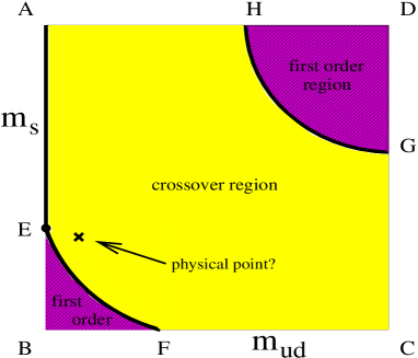
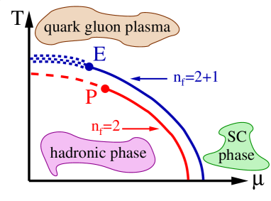
Figure 1: Left: the QCD phase diagram in the $m_{ud},m_{s}$ plane The thick solid lines represent second order transitions separating cross-over regions from first order ones. Right: the QCD phase diagram in the $\mu,T$ plane. In the case of two massless flavors, a second order region (dashed line) is connected to a first order region via the tricritical point ($P$). In the realistic case of two light and one heavier flavor, a crossover (dotted region) is connected to the first order region via the critical endpoint ($E$).

1.2 The QCD phase transition

At high temperature ($T$) and/or large chemical potential ($\mu$) the hadronic matter undergoes a transition into a quark-gluon dominated phase. At zero $\mu$ this transition happens at $T\approx 270$ MeV in the quenched case while at $T\approx 150-170$ MeV in full QCD. In the pure gauge case the action has an exact $Z(3)$ symmetry which is spontaneously broken in the low temperature phase. The Polyakov loop ($L$) is not invariant under this symmetry, thus it is an order parameter of the phase transition. In massless dynamical QCD we have chiral symmetry, which is expected to be broken in the low temperature phase. Correspondingly, the chiral condensate behaves as an order parameter in this case. In the realistic case with nonzero quark masses none of these symmetry breakings characterize the transition, nevertheless usually both the Polyakov loop and the chiral condensate shows a rapid change (or discontinuity) around the transition.

The transition can be usually located by observing the change of these order parameter-like quantities. Usually their susceptibilities show a nice signal which can be used as a definition of the transition point. An alternative possibility is to locate the Lee-Yang zeroes of the partition function [3]. This gives usually more precise values for $T_{c}$.

An interesting and natural question is, whether the transition is of first order, second order or maybe only a rapid cross-over. As lattice simulations are always done on lattices with a finite volume ($V$) where no singularities, thus no real phase transitions may occur, the only way to determine the order of the transition is to examine the finite size scaling behavior of certain observables, like the susceptibility peaks, Binder cumulants or the imaginary parts of Lee-Yang zeroes.

The phase diagram of QCD in the plane of the quark masses is shown in Fig. 1 (left). Based on universality arguments, one expects a first order phase transition for three flavors of massless quarks and a second order one for two massless flavors. In the quenched limit with infinite quark masses the transition is of first order as well. At nonzero, but finite quark masses the picture is more complicated. For intermediate masses we expect only a crossover. Whether the physical point lies within the first-order or cross-over region, is still an open question, however the cross-over is much more likely.

In the latter case an interesting picture emerges if we introduce a nonzero chemical potential ($\mu$). At zero temperature and large enough $\mu$ one expects a strong first order phase transition. If there is only a cross over at zero $\mu$ and finite $T$ then there should be a critical endpoint on the line connecting the two regions as seen in Fig. 1 (right). This endpoint is an unambiguous non-perturbative prediction of the QCD Lagrangian and has important experimental signatures [4].

            

Figure 2: Left: the continuum extrapolation of $T_{c}/\sqrt{\sigma}$ in the pure SU(3) theory using standard and RG-improved actions. Right: the pressure and energy density as a function of the temperature for standard and RG-improved actions.

1.3 The equation of state along the line of constant physics

Besides finding the transition temperature (which may be not even well defined in the case of a cross-over) and/or giving the phase diagram in the $\mu-T$ plane, one can also give the equation of state (EoS) of hadronic/gluonic matter well below or above the transition $T$,or $\mu$. All thermodynamical quantities can be obtained from the grand canonical partition function, e.g. for the energy density and the pressure:

$$\epsilon(T)=\frac{T^{2}}{V}\frac{\partial(\log Z)}{\partial{T}}\;\;\;p(T)=T\frac{\partial(\log Z)}{\partial V}.$$ (1)

On lattices with isotropic couplings we can not take derivatives with respect to $T$ and $V$ independently, as they are connected via the lattice spacing ($a$). The combination $\epsilon-3p$ can be written using derivatives with respect to $a$:

$$\frac{\epsilon-3p}{T^{4}}=-\frac{L_{t}^{3}}{L_{s}^{3}}\left\{a\frac{d(\log Z)}{da}-\mu\frac{d(\log Z)}{d\mu}\right\},$$ (2)

which can be rewritten in terms of the Plaquette ($P$) and chiral condensate ($\bar{u}u$ and $\bar{s}s$) expectation values:

$$\frac{\epsilon-3p}{T^{4}}=-L_{t}^{4} \left[a\frac{\partial\beta}{\partial a}<{\rm P}>+a\frac{\partial(am_{u})}{\partial a}<\bar{u}u>\right.$$ (3)

$$+\left.a\frac{\partial(am_{s})}{\partial a}<\bar{s}s>\right].$$

Here all derivatives should be taken along the line of constant physics (LCP) where the physical values of the quark masses (and not the $am_{i}$ lattice masses) are kept constant. In order to determine both $\epsilon$ and $p$ one needs another combination, which can be the pressure itself. For large homogeneous systems, $p\propto\log Z$, which can be computed using the integral method:

$$\frac{p}{T^{4}}=L_{t}^{4}\int d\beta\left[<{\rm P}>+m_{u}\frac{\partial a}{\partial\beta}<\bar{u}u>\right.$$

$$+\left.m_{s}\frac{\partial a}{\partial\beta}<\bar{s}s>+\mu\frac{\partial a}{\partial\beta}\frac{\partial(\log\det M)}{\partial(\mu a)}\right].$$ (4)

Here again the integration should follow the LCP and the subtraction of $T=0$ observables are assumed.

In the rest of this review recent results of lattice QCD at finite $T$ and/or $\mu$ are summarized. In the next section quenched results are reviewed. Sect. 3 deals with results of dynamical simulations using Wilson, staggered or overlap fermions. In sect. 4 the recent progress of exploring the $\mu\neq 0$ regions of the QCD phase diagram is discussed. Sect. 5 shortly introduces some QCD-like models used for studying large chemical potentials and finally, sect. 6 concludes.

              

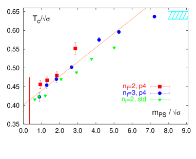
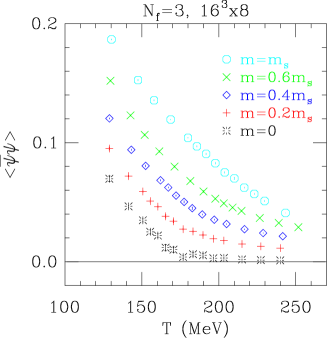
Figure 3: Left: the chiral extrapolation of $T_{c}/\sqrt{\sigma}$ for $N_{f}=2$ (squares), 3 (circles) for the $p4$ and $N_{f}=2$ (triangles) for the standard staggered action. Right: the chiral condensate as a function of the temperature for several quark masses and extrapolated to $m=0$ with $N_{f}=3$ ASQTAD fermions.

2 PURE GAUGE RESULTS

The simplest case to study is pure SU(3) gauge theory without dynamical quarks. Using both standard [5] and improved actions [6, 7] on isotropic and anisotropic [8] lattices the critical temperature has been determined in the continuum limit (see Fig. 2 left). The results are usually given in units of the string tension and one gets $T_{c}/\sqrt{\sigma}\approx 0.630-0.650$. The results seem to be not completely consistent, however the difference comes from possible systematic errors in measuring the string tension. If one sets the scale using the $r_{0}$ parameter [9] then a perfect agreement is found [10]. The equation of state is shown on Fig. 2 (right) for both actions. As the only parameter here is the gauge coupling which is used to set the scale, the system is kept automatically on the LCP. We can see that even at temperatures as high as $4T_{c}$ there is still 15% deviation from the Stefan-Boltzmann (SB) free gas limit. A careful finite size scaling analysis shows that the transition is of first order as expected [11].

3 DYNAMICAL RESULTS AT $\mu=0$

Including dynamical quarks increases the cost of simulations by at least two orders of magnitude. Another difficulty is introduced by the quark masses. As direct simulations at the physical values of the u,d quark masses are still practically impossible, chiral extrapolation is usually performed from larger masses. Taking the continuum limit is very expensive and it is usually not yet done. Therefore we still have to wait for final results.

3.1 Staggered results for $T_{c}$ and the EoS

The staggered discretization of the fermionic action describes four flavors of quarks with equal masses. Taking a fractional power of the fermion determinant one can also introduce less flavors. Using staggered fermions is significantly faster than Wilson fermions and another advantage is that part of the chiral symmetry is preserved. Fig. 3 (left) shows the results of the Bielefeld-group on $T_{c}$ using $p4$ action and $16^{3}\times 4$ lattices [12]. The critical points were defined by susceptibility peaks. The critical temperature on these $N_{t}=4$ lattices in the chiral limit is $T_{c}\approx 150(170)$ MeV for two (three) flavors. The MILC collaboration has somewhat different results using the ASQTAD action with 2+1 and 3 flavors [13] (Fig. 3 right). On $16^{3}\times 8$ lattices they see a weak crossover at somewhat larger $T_{c}\approx 180$ MeV. Note, that although they have a larger $N_{t}$, the volume they use is much smaller than the one used by the Bielefeld group. Thus, there may still be significant finite-size effects. Clearly, in order to have a reliable prediction for $T_{c}$ one has to take the thermodynamical limit and carry out a continuum extrapolation.

Both of these analyses used degenerate $u,d$ quark masses. It has been investigated in [14] that breaking the flavor SU(2) symmetry and using somewhat different $u,d$ masses does not change $T_{c}$ significantly.

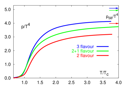
Figure 4: The pressure as a function of $T/T_{c}$ for $N_{f}=3,2+1,2$ (from top to bottom) $p4$ fermions.

Using standard staggered action the equation of state has been determined by the MILC collaboration [15] on $N_{t}=4$ and 6. Fig. 4 shows the pressure obtained by the Bielefeld group with $p4$ action on $16^{3}\times 4$ lattices [16].

Note that both analyses kept $am_{q}$ constant which is not an LCP approach as discussed in the introduction. In these cases the physical quark masses increase as the temperature is increased. This leads to a 10-15% suppression of the pressure at high temperatures compared to the LCP approach [17].

         

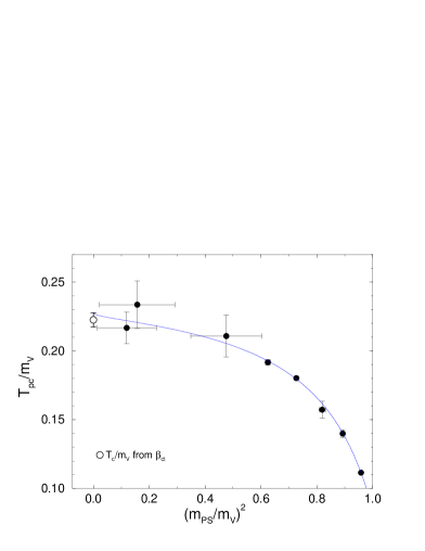
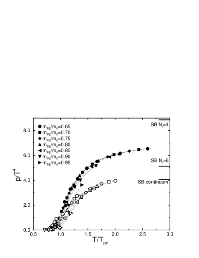
Figure 5: Left: the chiral extrapolation of $T_{c}/m_{V}$ using improved Wilson fermions. Right: the pressure for different quark masses on $N_{t}=4$ and $N_{t}=6$ lattices.

3.2 Results with Wilson fermions

There are numerous results for $T_{c}$ using Wilson quarks [18, 19, 20, 21]. Fig. 5 (left) shows the chiral extrapolation of $T_{c}$ normalized by the vector boson mass as obtained by the CP-PACS collaboration [20] using RG improved gauge- and clover improved Wilson action on $N_{t}=4$ lattices. The chirally extrapolated result is $T_{c}=171(4)$ MeV, similarly to previously discussed staggered results.

The equation of state as obtained in [22] is shown in Fig. 5 (right) for $N_{t}=4$ and $6$ lattices. This analysis was carried out along the LCP.

3.3 First results with overlap fermions

As the chiral properties of the action may be important when we investigate the chiral phase transition in the massless limit there would be a need to have thermodynamics with chiral fermions, i.e. with ones satisfying the Ginsparg-Wilson relation [23]. One possible realization is the Overlap formalism [24]. Unfortunately due to the non-analytic form of the Overlap operator, all simulations are computationally extremely expensive. In fact, no dynamical simulations have been performed before.

As an exploratory study we implemented the standard hybrid Monte-Carlo algorithm for the overlap operator [25]. The sign function was approximated by the Zolotarev optimal rational polynomial approximation [26]. In this approximation one has to perform simultaneous inversions which is done with a multi-shift solver [27]. As it was expected, the computational costs are more than two orders of magnitude higher than for dynamical Wilson fermions.

The first results on a $6^{3}\times 4$ lattice are shown in Fig. 6. The Polyakov loop shows a clear transition behavior. This result can of course be considered only as a demonstration of the working algorithm, for real physical results much larger lattices with smaller lattice spacings are required.

3.4 The order of the transition

As it has been emphasized in the introduction, the order of the phase transition can only be determined by a careful finite-size scaling analysis. In the case of dynamical simulations these analyses have given little results yet. For $N_{f}=2$ in the massless limit one expects a second order phase transition in the O(4) universality class. However, only simulations with improved Wilson quarks could support this expectation [20]. Staggered results do not seem completely consistent with O(4) universality [28, 29, 30].

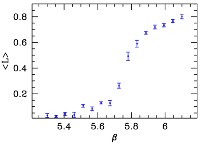
Figure 6: The Polyakov loop as a function of the $\beta$ coupling using dynamical overlap fermions on a $6^{3}\times 4$ lattice.

In the case of three degenerate flavors a first order transition is expected at zero quark masses. Thus if we increase the quark masses, we will have a critical $m_{c}$ (and correspondingly a critical pseudoscalar mass, $m_{PSc}$) where the first order transition ends. This second order endpoint has been located in standard staggered QCD on $N_{t}=4$ lattices [31] and the critical mass is $m_{PSc}\approx 290$ MeV. However, using improved $p4$ fermions, this critical mass goes down $m_{PSc}\approx 67$ MeV [32] indicating that there are still large cutoff effects. The picture in the physically interesting $N_{f}=2+1$ case is even more unclear, however it is very likely that there is only a rapid cross-over [33].

3.5 Heavy quark free energy and hadron properties

One can study the heavy quark free energy at finite temperatures by measuring the correlation of Polyakov loops:

$$<L_{x}L^{\dagger}_{y}>\sim e^{-V(|x-y|,T)/T}$$ (5)

As an effect of dynamical quarks, string breaking is expected at large separations. This string breaking happens at 2-3 times smaller distances as we are getting closer to the critical temperature [34, 35]. The asymptotic value of the free energy at large separations shows a strong temperature and quark mass dependence. As it is expected, for larger temperatures and smaller quark masses the asymptotic value gets smaller.

Measuring hadron masses is not easy at finite $T$, since the temporal extension of the lattice is small. One can either use anisotropic lattices or measure spatial correlators leading to screening masses [36, 37].

A recent development is the possibility of reconstructing spectral functions from the Euclidean correlation functions using the Maximal Entropy Method (MEM) [38]. For a good determination, however a large $N_{t}$ is required. Quenched results are already available both for anisotropic lattices up to $N_{t}=54$  [39] and isotropic lattices up to $N_{t}=32$ [40].

4 QCD AT FINITE, BUT SMALL $\mu$

Unlike at finite $T$ but zero $\mu$, at finite chemical potentials the strategy of lattice simulations is not well defined. The reason is that at nonzero $\mu$ the fermion determinant becomes complex which spoils direct importance-sampling based simulations.

Recently several methods have been developed to extract information for finite $\mu$ from simulations at zero or purely imaginary $\mu$ values where the fermion determinant is positive definite. These techniques are, however still restricted to finite $T$ and relatively small $\mu$. The validity region is approximately $\mu\mbox{\,\raisebox{1.29167pt}{$<$}$\!\!\!\!\!$\raisebox{-3.87495pt}{$\sim$}\,}T$. At larger chemical potentials, especially at low temperature, the only current possibility is to use QCD-like effective models which reflect certain properties of QCD and which can be solved either exactly or by numerical techniques. Some of these models will be discussed in the next section.

4.1 Multiparameter reweighting

Figure 7: The phase diagram of QCD from $N_{f}=2+1$ simulations on $N_{t}=4$ lattices. The dotted part on the left represents a crossover which is separated from the first-order line via the critical endpoint.

One of the possibilities to extract information at $\mu\neq 0$ is the Glasgow method [41]. It is based on a reweighting in $\mu$. An ensemble is generated at $\mu=0$ and the ratio of the fermion determinants at finite $\mu$ and $\mu=0$ is taken into account as an observable. This method was used to attempt to locate the phase transition at low $T$ and finite $\mu$, however it fails even on lattices as small as $4^{4}$. The reason is the so-called overlap problem. The generated configurations (only hadronic ones) do not have enough overlap with the configurations of interest (e.g. in the case of a phase transition a mixture of hadronic and quark-gluon dominated ones).

A simple, but powerful generalization of the Glasgow method is the overlap improving multiparameter reweighting [42]. The partition function at finite $\mu$ can be rewritten as:

$$Z=\int{\cal D}Ue^{-S_{g}(\beta,U)}\det M(m,\mu,U)=$$

$$\int{\cal D}Ue^{-S_{g}(\beta_{0},U)}\det M(m_{0},\mu=0,U)$$ (6)

$$\left\{e^{-S_{g}(\beta,U)+S_{g}(\beta_{0},U)}\frac{\det M(m,\mu,U)}{\det M(m_{0},\mu=0,U)}\right\},$$

where the second line contains a positive definite action which can be used to generate the configurations and the terms in the curly bracket in the last line are taken into account as an observable. The expectation value of any observable can be then written in the form:

$$<O>_{\beta,m,\mu}=\frac{\sum O(\beta,m,\mu)w(\beta,m,\mu)}{\sum w(\beta,m,\mu)}$$ (7)

with $w(\beta,m,\mu)$ being the weights of the configurations defined by the curly bracket of eqn. (4.1).

The main difference from the Glasgow method is that reweighting is done not only in $\mu$ but also in the other parameters of the action (at least in $\beta$, but possibly also in $m$). This way the overlap can be improved. If the starting point ($\beta_{0},m_{0},\mu_{0}=0$) is selected to be at the $\mu=0$ transition point then a much better overlap can be obtained with transition points at higher $\mu$. One can in general define the best weight lines along which – starting from a given point ($\beta_{0},m_{0},\mu_{0}$) – the overlap is maximal. This can be done e.g. by minimizing the spread of the $w$ weights. An alternative way is to diagonalize the covariance matrices for infinitesimal steps [43]. It has been observed that starting from the $\mu=0$ transition point, the above defined best weight line coincides with the transition line [44].

An interesting question is the goodness of reweighting and its dependence on the simulation parameters, most importantly on the lattice volumes. One can define an overlap measure the following way: let the overlap measure be $2\alpha$ if $\alpha$ fraction of the configurations with largest weights (or their absolute values for complex weights) gives $1-\alpha$ fraction of the total weight. Clearly for true important sampling, when all the weights are 1, this definition gives 1 for the overlap measure, otherwise it is smaller. If we require $2\alpha>1/2$ as a condition for acceptable reweighting, then the maximal reachable chemical potential, denoted by $\mu_{1/2}$ scales with the volume as $\mu_{1/2}\propto V^{-\gamma}$ with $\gamma=0.2-0.3$ from $6^{3}\times 4,8^{3}\times 4,10^{3}\times 4$ and $12^{3}\times 4$ lattice simulations [17]. If $\gamma<0.25$ then it has the important consequence that the continuum limit can be taken, as the chemical potential in lattice units we have to reach scales with $V^{-0.25}$.

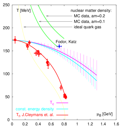
Figure 8: The phase diagram of QCD from $N_{f}=2$ simulations on $16^{3}\times 4$ lattices with $p4$ action using Taylor expansion [47].

This reweighting technique made it possible to determine the phase diagram on the $\mu-T$ plane up to $\mu\approx 1.5T$ in $N_{f}=4$  [42] and $N_{f}=2+1$ [45] staggered QCD on $N_{t}=4$ lattices. The transition points were located in both cases by finding the Lee-Yang zeroes of the partition function.

In the $N_{f}=2+1$ case, as discussed in the introduction, there is a possibility to have a critical endpoint at finite $\mu_{E},T_{E}$ values. Indeed, the finite size scaling behavior of the imaginary parts of the Lee-Yang zeroes indicated a cross-over at $\mu=0$ and this turned into a first-order transition at larger $\mu$ values. After setting the scale with $T=0$ simulations, the temperature and baryonic chemical potential ($\mu_{B}=3\cdot\mu$) at the endpoint can be given in physical units:

$$T_{E}=160\pm 3.5{\rm MeV},\;\;{\mu_{B}}_{E}=725\pm 35{\rm~{}MeV}.$$ (8)

The phase diagram and the endpoint is shown on Fig. 7. Note that a similar two-parameter reweighting was succesfully applied to locate the endpoint of the electroweak phase transition even on large lattices [46].

4.2 Multiparameter reweighting with Taylor-expansion

The use of eqn. (4.1) requires the exact calculation of determinants on each gauge configuration which is computationally very expensive. Instead of using the exact formula, one can make a Taylor expansion for the determinant ratio in the weights [47] (for simplicity assuming no reweighting in the mass):

$$\ln\left(\frac{\det M(\mu)}{\det M(0)}\right) = \sum_{n=1}^{\infty}\frac{\mu^{n}}{n!}\frac{\partial^{n}\ln\det M(0)}{\partial\mu^{n}}$$ (9)

$$\equiv \sum_{n=1}^{\infty}{R}_{n}\mu^{n}.$$

Taking only the first few terms of the expansion one gets an approximate reweighting formula. The advantage of this approximation is that the coefficients are derivatives of the fermion determinant at $\mu=0$, which can be well approximated stochastically. However, due to the termination of the series and the errors introduced by the stochastic evaluation of the coefficients we do not expect this method to work for as large $\mu$ values as the full technique. Indeed, it has been shown in [48] that even for very small lattices (i.e. $4^{4}$) the phase of the determinant is not reproduced by the Taylor expansion for $a\mu>=0.2$.

Fig. 8 shows the phase diagram of $N_{f}=2$ QCD determined on $16^{3}\times 4$ lattices with $p4$ action using this Taylor-expansion technique [47]. The results are consistent with the above ones coming from the full technique.

               

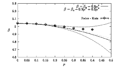
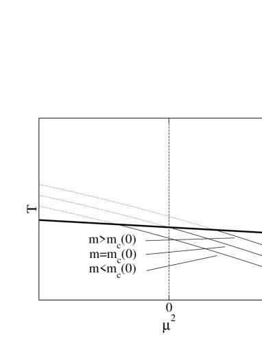
Figure 9: Left: the phase diagram of QCD from $N_{f}=4$ simulations at imaginary $\mu$ with staggered fermions [50]. Right: schematic plot of the phase diagrams (the dotted parts are cross-over while the solid parts first order regions) for different quark masses and the line of endpoints (thick solid line).

As discussed in the previous section $N_{f}=3$ QCD has a critical quark mass at which there is a second order endpoint at $\mu=0$. If we make reweighting also in the quark masses then we can keep the system not only on the transition line, but also on a critical surface. This way in principle the critical endpoint at the physical values of the quark masses can be determined [32].

4.3 Simulations at imaginary $\mu$

The fermion determinant is positive definite if we use a purely imaginary chemical potential. So if the transition line $T_{c}(\mu)$ is an analytic function then we can determine it for imaginary $\mu$ values and analytically continue back to real $\mu$-s. The analytic continuation is in general impossible from just a finite number of points. However, taking a Taylor expansion in $\mu$ or $\mu/T$ one gets:

$$\frac{T_{c}(\mu_{B})-T_{c}(0)}{T}=a_{2}\left(\frac{\mu_{B}}{T}\right)^{2}+a_{4}\left(\frac{\mu_{B}}{T}\right)^{4}+\dots$$ (10)

The coefficients $a_{i}$ can be determined from imaginary $\mu$ simulations. One simply measures $T_{c}(\mu_{I})$ for imaginary $\mu_{I}$-s and fits it with a finite order polynomial in $\mu_{I}/T$. This method has been applied for $N_{f}=2$ [49] ,$N_{f}=4$ [50] and recently for $N_{f}=3$ [51] staggered QCD on $N_{t}=4$ lattices. The $N_{f}=4$ results are shown on Fig. 9 (left). The curvatures of the phase diagram in the three cases are $a_{2}$=-0.0056, -0.011 and -0.0068. The $a_{4}$ coefficient is very small and it can only be distinguished from zero with very high statistics [51].

Similarly to the case of reweighting one can study the mass dependence of the $\mu_{E}$ endpoint. In $N_{f}=3$ QCD for quark masses below the critical value this endpoint is at imaginary values of $\mu$ (i.e. negative $\mu^{2}$), which can be investigated. If one assumes the same leading order dependence on $m$ also for real values of $\mu$ (i.e. positive $\mu^{2}$) one can in principle determine the location of the critical endpoint for the physical values of the quark masses (c.f. Fig. 9 right). The first steps have been made in [51] and the critical line in the $\mu-m$ plane has been found for 3 degenerate quarks:

$$\frac{m_{c}(\mu)}{m_{c}(\mu=0)}=1+0.84(36)\left(\frac{\mu}{\pi T}\right)^{2}$$ (11)

4.4 The EoS at finite $\mu$

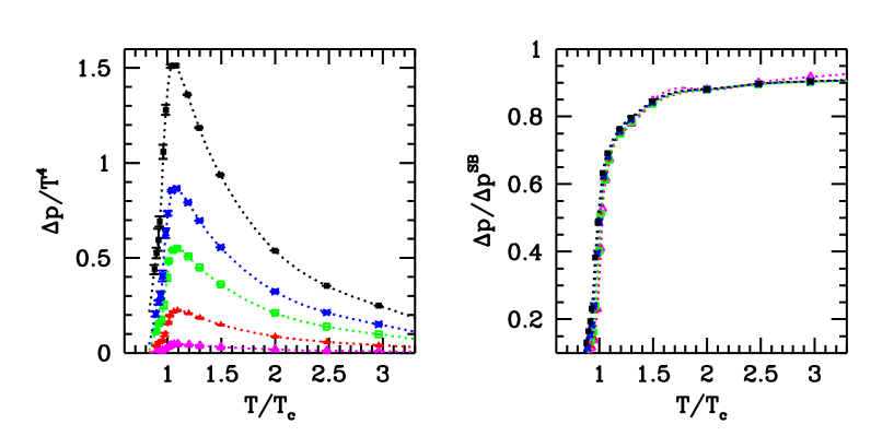
Figure 10: Left: The pressure difference $\Delta p=p(\mu)-p(0)$ for baryonic chemical potentials $mu_{B}=100,210,330,410,530$ MeV (from bottom to top) obtained with $N_{f}=2+1$ staggered QCD on $N_{t}=4$ lattices. Right: $\Delta p$ normalized by the Stefan-Boltzmann limit.

If we perform reweighting not only along the transition line but also below or above it, following the above defined best weight lines then the equation of state can be given at finite $\mu$. For calculating the pressure or the energy density one simply has to follow the formulae of the introduction, but all observables have to be reweighted to finite $\mu$ according to eqn.(7). Calculating the pressure is done by a line integral in the $\beta-\mu$ plane. The simplest choice for the integration path is to start from deep in the hadronic phase (where we get zero contribution after subtracting the $T=0$ contributions) then integrate up to some $\beta_{1}$ at $\mu=0$ and then follow a best weight line.

Keeping the system always on the LCP is an important aspect of the EoS. However, if we make reweighting only in $\beta$ and $\mu$ then following the best weight lines change $\beta$ but not $am_{i}$, so we automatically leave the LCP. There are two possible solutions. One could either use also a reweighting in $m_{i}$, which makes all computations more expensive, or start the reweighting from two different LCP-s and then keep the system on the LCP with an appropriate interpolation. The second technique was used in [52] where the EoS was determined for a large range in $T$ and $\mu$. The results for the pressure are shown in Fig. 10. The left panel shows the pressure after subtracting the $\mu=0$ contribution. On the right panel the pressure is normalized with the Stefan-Boltzmann limit. We can observe an almost universal scaling behavior. After this normalization the pressure becomes practically independent of $\mu$ in the analyzed region. One can get similar results using a quasi-particle picture, after setting the free parameters of the model using $\mu=0$ lattice results [53].

         

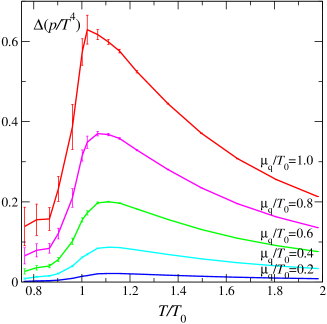
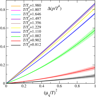
Figure 11: Left: The pressure difference $\Delta p=p(\mu)-p(0)$ using the Taylor expansion method with $N_{f}=2$ staggered QCD with $p4$ action on $N_{t}=$ lattices. Right: $\Delta p$ as a function of $\mu$ for different $T$-s.

The EoS can also be determined using Taylor expansion. The pressure can be written as:

$$\frac{p}{T^{4}}(\mu,T)=\frac{p_{0}(T)}{T^{4}}+c_{2}\left(\frac{\mu}{T}\right)^{2}+c_{4}\left(\frac{\mu}{T}\right)^{4}+\dots$$ (12)

The coefficients can be determined with simulations at $\mu=0$. Fig. 11 shows the results from this method [54], which are very similar to those coming from the full technique. In the vicinity of the critical endpoint the nonlinear susceptibility, $c_{4}$ diverges. Thus the convergence radius of the $p(\mu,T)$ function in principle gives the location of the endpoint. One can estimate this convergence radius by the ratios of the subsequent coefficients.

The pressure has also been computed with the help of eqn.(12) using quenched configurations [55].

Simulations at imaginary $\mu$ can also be used to determine the $c_{i}$ coefficients. A first analysis was presented in [56].

4.5 The factorization method

Although it has not yet been tested for QCD, the factorization method [57] seems very promising, so we discuss it in this subsection. The factorization method was used to study an exactly solvable random matrix model defined by:

$$Z=\int dWe^{-N{\rm Tr}(W^{\dagger}W)}\det D$$ (13)

with $W$ being $N\times N$ complex matrices and

$$D=\left(\begin{array}[]{cc}m&iW+\mu\\ iW^{\dagger}+\mu&m\end{array}\right)$$ (14)

For $\mu\neq 0$ the determinant is complex as in QCD. The main idea of the factorization method is to use constrained partition functions:

$$Z_{\nu}(x)=\int dWe^{-S}|detD|\delta(x-\nu)$$ (15)

with some real-valued observable $\nu$. If one performs simulations at several $x$ values using $Z_{\nu}(x)$ and includes the phase of the determinant as an observable then after integrating over $x$ one can get $<\nu>$ for the full theory. The advantage of this approach is that each value of the observable is sampled with the help of $Z_{\nu}(x)$ thus solving the overlap problem. One disadvantage is of course the need of simulations at several $x$ values and that for each observable an independent simulation is needed. The implementation of $Z_{\nu}(x)$ for QCD especially for the most interesting fermionic observables (e.g. quark density) is also not trivial. However, as this method produced results completely consistent with the exact ones for this simple random matrix theory [57], we could expect similar success for QCD. The technique is not expected to work at large $\mu$ because a reweighting is still needed to include the phases of the determinant and when they become strongly oscillating this may make the measurement of the observables even with the constrained partition functions impossible.

5 QCD-LIKE MODELS

At low temperature and large densities a rich phase structure of QCD is conjectured. Due to asymptotic freedom at large densities quarks are expected to be weakly coupled. However, as there is still a weak attractive interaction they can form Cooper-pairs and thus break the SU(3) symmetry spontaneously and lead to color superconductivity. It is also expected that the ground state will be a color-flavor locked (CFL) phase.

Unfortunately these regions are still unavailable for lattice simulations due to the overlap problem and the strong oscillation of the phase of the fermion determinant. One can, however study QCD-like models, which have positive actions and which are expected to reproduce some features of high density QCD. In the following we briefly discuss the most widely used models to study high density phenomena.

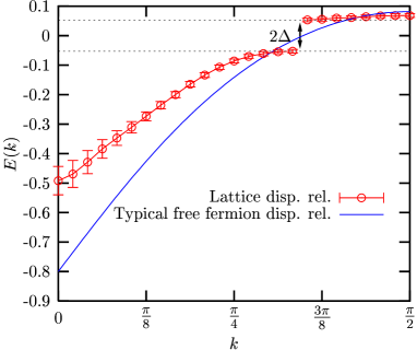
Figure 12: The energy-momentum dispersion relation for the 3+1 dimensional NJL model. The energy gap can be seen clearly.

5.1 Two color QCD

QCD with two colors has a real fermion determinant, which is also positive definite for an even number of flavors even at nonzero chemical potential. Thus its properties can be studied on the whole $\mu-T$ plane with standard Monte-Carlo methods. Phase transitions have been observed both at finite $T$ and $\mu=0$ and at low $T$ and finite $\mu$ [58, 59]. An interesting property of two-color QCD that it also has an endpoint in the $\mu-T$ plane so it can be used to test any method which is used to locate the endpoint of real QCD.

Unfortunately there is no Fermi surface in this model, so it can not be used to study superconductivity.

The modification of hadron properties due to the chemical potential has also been investigated in this model [60].

5.2 Isospin chemical potential

If we introduce opposite chemical potentials for the $u$ and $d$ quarks then the phases of their fermion determinants cancel, so QCD with such an isospin $\mu$ has a positive definite action. This model has been studied in detail recently [61]. Interestingly at low densities it behaves very similarly to QCD with real chemical potential, which leads to the conclusion that at finite $T$ and low density the phase of the fermion determinant does not play an important role. On the other hand, at low temperatures, just as expected, a phase transition happens at $\mu\approx m_{\pi}/2$, as the pions are the lowest excitations in this system. This transition should not be present in QCD with baryonic $\mu$.

As in the case of two-color QCD, Fermi phenomena can not be studied in this model.

5.3 Four-fermion models

In principle one could integrate out the gauge fields in QCD leading to en effective purely fermionic theory. The first non-trivial interaction term of such an effective theory is a four-fermion interaction. Thus, models with four-fermion interactions are expected to reflect some features of QCD.

The 2+1 dimensional Gross-Neveu model has been studied in [62]. Fermi phenomena have been observed, however no gap was found in the energy-momentum dispersion relations. The non-exponential decay of meson correlation functions indicate the existence of massless particle-hole excitations.

The NJL model was studied both in 2+1 [63] and 3+1 [64] dimensions. Interestingly due to the different dimensionalities the two models behave differently in the large density regions. While in both models a $qq$ pairing has been observed, only the latter system shows BCS condensation and an energy gap in the dispersion relation (see Fig. 12). Unfortunately this 3+1 dimensional model is not renormalizable, however using a finite cutoff, one can set the parameters of the theory to describe low-energy observables of QCD.

5.4 Low energy effective models

Although the action of QCD at large densities is complex, it has been shown in [65] that if one is only interested in the low energy behavior, i.e. modes close to the Fermi surface, then a low-energy effective action can be derived which is positive definite (see also [66]). Using this low energy effective action it has been proven that the CFL phase is the ground state of QCD at large densities.

Another approach is to build up an effective Hamiltonian based on strong coupling expansion, which can then be used to study phenomena even in the chiral limit [67].

6 CONCLUSIONS

In this review recent results of lattice QCD at finite $T$ and/or $\mu$ have been discussed. For the pure gauge theory there are already continuum-extrapolated predictions both for the phase transition temperature and the equation of state. The transition is proven to be first order.

Including dynamical quarks makes all computations much more complicated. Therefore there are still no chiral- and continuum-extrapolated results. However, the transition temperature, the equation of state, the heavy quark potential and hadron properties are quite well known and all necessary, but still missing extrapolations can be expected in the near future.

The case of finite $\mu$ is even more complicated due to the complexness of the action. The exploration of the phase diagram, the critical endpoint and the equation of state has just began recently. Lots of new results can be expected in the near future especially in the small $\mu$ region.

Unfortunately even the latest methods are still incapable of solving the complex action problem which is most severe for the very interesting large $\mu$, small $T$ region. Therefore effective, QCD-like models are used to investigate this parameter region. These effective models seem to support the assumption on the existence of a color-superconducting phase at large densities.

7 ACKNOWLEDGMENTS

I thank Zoltán Fodor for many useful discussions and for careful reading of the manuscript.

References

- [1] L. D. McLerran and B. Svetitsky, Phys. Lett. B 98 (1981) 195.
- [2] J. Kuti, J. Polonyi and K. Szlachanyi, Phys. Lett. B 98 (1981) 199.
- [3] C. N. Yang and T. D. Lee, Phys. Rev. 87 (1952) 404; Phys. Rev. 87 (1952) 410.
- [4] M. A. Stephanov, K. Rajagopal and E. V. Shuryak, Phys. Rev. Lett. 81 (1998) 4816.
- [5] G. Boyd, J. Engels, F. Karsch, E. Laermann, C. Legeland, M. Lutgemeier and B. Petersson, Nucl. Phys. B 469 (1996) 419.
- [6] B. Beinlich, F. Karsch, E. Laermann and A. Peikert, Eur. Phys. J. C 6 (1999) 133.
- [7] M. Okamoto et al. [CP-PACS Collaboration], Phys. Rev. D 60 (1999) 094510.
- [8] Y. Namekawa et al. [CP-PACS Collaboration], Phys. Rev. D 64 (2001) 074507.
- [9] R. Sommer, Nucl. Phys. B 411 (1994) 839.
- [10] S. Necco, hep-lat/0309017.
- [11] M. Fukugita, M. Okawa and A. Ukawa, Phys. Rev. Lett. 63 (1989) 1768.
- [12] F. Karsch, E. Laermann and A. Peikert, Nucl. Phys. B 605 (2001) 579.
- [13] C. Bernard et al. [MILC Collaboration], hep-lat/0309118.
- [14] R. V. Gavai and S. Gupta, Phys. Rev. D 66 (2002) 094510.
- [15] C. W. Bernard et al. [MILC Collaboration], Phys. Rev. D 55 (1997) 6861 hep-lat/9612025].
- [16] F. Karsch, E. Laermann and A. Peikert, Phys. Lett. B 478 (2000) 447.
- [17] F. Csikor, G.I. Egri, Z. Fodor, S.D. Katz, K.K. Szabo, A.I. Toth, in preparation.
- [18] C. W. Bernard et al., Phys. Rev. D 46 (1992) 4741.
- [19] R. G. Edwards and U. M. Heller, Phys. Lett. B 462 (1999) 132.
- [20] A. Ali Khan et al. [CP-PACS Collaboration], Phys. Rev. D 63 (2001) 034502.
- [21] Y. Mori et al., Nucl. Phys. A 721 (2003) 930 hep-lat/0301003].
- [22] A. Ali Khan et al. [CP-PACS collaboration], Phys. Rev. D 64 (2001) 074510.
- [23] P. H. Ginsparg and K. G. Wilson, Phys. Rev. D 25 (1982) 2649.
- [24] H. Neuberger, Phys. Lett. B 417 (1998) 141.
- [25] Z. Fodor, S.D. Katz and K.K. Szabo, in preparation.
- [26] J. van den Eshof, A. Frommer, T. Lippert, K. Schilling and H. A. van der Vorst, Comput. Phys. Commun. 146 (2002) 203; T. W. Chiu, T. H. Hsieh, C. H. Huang and T. R. Huang, Phys. Rev. D 66 (2002) 114502.
- [27] A. Frommer, B. Nockel, S. Gusken, T. Lippert and K. Schilling, Int. J. Mod. Phys. C 6 (1995) 627.
- [28] S. Aoki et al. [JLQCD Collaboration], Phys. Rev. D 57 (1998) 3910.
- [29] C. W. Bernard et al., Phys. Rev. D 61 (2000) 054503.
- [30] J. Engels, S. Holtmann, T. Mendes and T. Schulze, Phys. Lett. B 514 (2001) 299.
- [31] F. Karsch, E. Laermann and C. Schmidt, Phys. Lett. B 520 (2001) 41.
- [32] F. Karsch, C. R. Allton, S. Ejiri, S. J. Hands, O. Kaczmarek, E. Laermann and C. Schmidt, hep-lat/0309116.
- [33] C. Schmidt, C. R. Allton, S. Ejiri, S. J. Hands, O. Kaczmarek, F. Karsch and E. Laermann, hep-lat/0209009.
- [34] V. Bornyakov et al., hep-lat/0301002.
- [35] O. Kaczmarek, F. Karsch, P. Petreczky and F. Zantow, hep-lat/0309121.
- [36] E. Laermann and P. Schmidt, Eur. Phys. J. C 20 (2001) 541.
- [37] R. V. Gavai and S. Gupta, Phys. Rev. D 67 (2003) 034501.
- [38] M. Asakawa, T. Hatsuda and Y. Nakahara, Prog. Part. Nucl. Phys. 46 (2001) 459.
- [39] M. Asakawa, T. Hatsuda and Y. Nakahara, Nucl. Phys. A 715 (2003) 863.
- [40] F. Karsch, E. Laermann, P. Petreczky and S. Stickan, Phys. Rev. D 68 (2003) 014504; P. Petreczky, S. Datta, F. Karsch and I. Wetzorke, hep-lat/0309012.
- [41] I. M. Barbour, S. E. Morrison, E. G. Klepfish, J. B. Kogut and M. P. Lombardo, Nucl. Phys. Proc. Suppl. 60A (1998) 220.
- [42] Z. Fodor and S. D. Katz, Phys. Lett. B 534 (2002) 87.
- [43] P. R. Crompton, Nucl. Phys. B 619 (2001) 499.
- [44] S. Ejiri, hep-lat/0212022.
- [45] Z. Fodor and S. D. Katz, JHEP 0203 (2002) 014.
- [46] F. Csikor, Z. Fodor and J. Heitger, Phys. Rev. Lett. 82 (1999) 21.
- [47] C. R. Allton et al., Phys. Rev. D 66 (2002) 074507.
- [48] P. de Forcrand, S. Kim and T. Takaishi, hep-lat/0209126.
- [49] P. de Forcrand and O. Philipsen, Nucl. Phys. B 642 (2002) 290.
- [50] M. D’Elia and M. P. Lombardo, Phys. Rev. D 67 (2003) 014505.
- [51] P. de Forcrand and O. Philipsen, hep-lat/0307020.
- [52] Z. Fodor, S. D. Katz and K. K. Szabo, Phys. Lett. B 568 (2003) 73.
- [53] K. K. Szabo and A. I. Toth, JHEP 0306 (2003) 008.
- [54] C. R. Allton, S. Ejiri, S. J. Hands, O. Kaczmarek, F. Karsch, E. Laermann and C. Schmidt, Phys. Rev. D 68 (2003) 014507.
- [55] R. V. Gavai and S. Gupta, Phys. Rev. D 68 (2003) 034506.
- [56] M. D’Elia and M. P. Lombardo, hep-lat/0309114.
- [57] J. Ambjorn, K. N. Anagnostopoulos, J. Nishimura and J. J. Verbaarschot, JHEP 0210 (2002) 062.
- [58] S. Hands, I. Montvay, S. Morrison, M. Oevers, L. Scorzato and J. Skullerud, Eur. Phys. J. C 17 (2000) 285.
- [59] J. B. Kogut, D. Toublan and D. K. Sinclair, Nucl. Phys. B 642 (2002) 181.
- [60] S. Muroya, A. Nakamura and C. Nonaka, Phys. Lett. B 551 (2003) 305.
- [61] J. B. Kogut and D. K. Sinclair, Phys. Rev. D 66 (2002) 034505.
- [62] S. Hands, J. B. Kogut, C. G. Strouthos and T. N. Tran, Phys. Rev. D 68 (2003) 016005.
- [63] S. Hands, B. Lucini and S. Morrison, Phys. Rev. Lett. 86 (2001) 753.
- [64] S. Hands and D. N. Walters, Phys. Lett. B 548 (2002) 196; hep-lat/0308030.
- [65] D. K. Hong and S. D. Hsu, Phys. Rev. D 68 (2003) 034011.
- [66] S. Hands, hep-ph/0310080.
- [67] Y. Z. Fang and X. Q. Luo, hep-lat/0210031.