Higher-order perturbation theory for highly-improved actions

Abstract

I review techniques and applications of higher-order perturbation theory for highly-improved lattice actions.

1 Introduction

Lattice QCD simulations are routinely done nowadays using highly-improved actions, which are designed to remove the leading errors arising from the discretization of the continuum theory. Improved actions can be designed from both perturbative and nonperturbative considerations. In this review I describe techniques for doing the higher-order perturbation theory (PT) calculations that are necessary in the design of highly-improved lattice discretizations for gluons, staggered quarks, and heavy quarks. Recent results obtained with these methods are also reviewed.

Much of the work described here is part of the program of the HPQCD collaboration, a major goal of which is to make precision calculations of hadronic matrix elements relevant to $b$-physics experiments. In order to fully realize the potential impact of these experiments on the parameters of flavor mixing requires calculations of the relevant hadronic matrix elements to a few percent accuracy. The CLEO-c program also presents an enormous opportunity to validate lattice QCD methods for $b$ physics, by testing predictions for analogous quantities in the charm system.

These stringent requirements for accuracy and timeliness are unlikely to be met without significant algorithmic developments, in both the efficiency of unquenched simulations, and in the technical challenges posed by lattice PT. The development of an improved action for staggered quarks [1, 2] has at last made accurate unquenched simulations feasible [3] at dynamical quark masses that are small enough to allow for reliable chiral extrapolations to the physical region [4]. This is one particularly striking success of the perturbative analysis of lattice discretizations. More generally one must do perturbative matching calculations for a wide array of coupling constants, action parameters and hadronic matrix elements.

The scope of the charge to lattice PT is set by two expansion parameters: $a\Lambda_{\rm QCD}$, where $a$ is the lattice spacing and $\Lambda_{\rm QCD}$ is a typical low-energy scale; and the strong coupling $\alpha_{s}(q^{*})$, evaluated near the ultraviolet cutoff ($q^{*}\sim 1/a)$ at which the lattice theories are to be matched onto continuum QCD. Affordable unquenched simulations can only be done for lattice spacings around 0.1 fm, where these two expansion parameters have about the same value:

$$\alpha_{s}(1/a)\approx a\Lambda_{\rm QCD}\approx 0.2\mbox{--}0.3\quad[a\approx 0.1~{}\mbox{fm}].$$ (1)

Hence to reduce systematic errors to a few percent requires lattice discretizations that are accurate through ${\cal O}(a^{2})$, which is trivial to do by numerical analysis, and matching of the resulting action and operators must be done through $O(\alpha_{s}^{2})$.

The latter requirement is highly nontrivial, and in fact only a few two-loop PT calculations in lattice QCD have ever been done. In many ways perturbative calculations with a lattice regulator are much more difficult than with dimensional regularization: the Feynman rules for lattice theories are exceedingly complicated, even for the simplest discretizations, with a tower of contact interactions that leads to a proliferation of Feynman diagrams that are not present in the continuum.

One has the challenge of doing many two-loop matching calculations, and doing these for the most complicated actions yet designed. Moreover one may anticipate further evolution in the actions that are actually used in simulations, as investigations continue into the optimal discretizations, hence one will want to be able to redo many perturbative calculations as the actions evolve.

Fortunately there exists several techniques which make higher-order lattice PT more manageable. In this review I survey two very different and somewhat complementary methods: one for conventional Feynman diagram evaluation of loop corrections, and another approach in which one does Monte Carlo simulations of the lattice path integral in the weak-coupling regime.

The linchpin of our program for diagrammatic PT is the automatic generation of the Feynman rules for lattice actions. This method was developed long ago by Lüscher and Weisz [5], and is described in Sect. 2. What is new in our work is that we have aggressively applied this method to higher-order calculations for highly-improved actions for gluons, staggered quarks, and heavy quarks. This is in order to analyze the MILC simulations of (2+1)-dynamical quark flavors [3], which were done for the $O(\alpha_{s}a^{2})$-accurate Symanzik gluon action, and the tree-level $O(a^{2})$-accurate staggered quark action due to Lepage [1], both with tadpole improvement.

A major effort of the past year has been devoted to a complete third-order determination of $\alpha_{s}(M_{Z})$, the first from lattice QCD, which should provide one of the most accurate determinations of the strong coupling. This requires a set of two- and three-loop calculations, which are described in Sects. 3 and 4.

Some other recent PT calculations are briefly reviewed in Sect. 5; a comprehensive review of recent work cannot be done in this short space, so I have mainly restricted this summary to work done with automated methods. Monte Carlo methods for the extraction of perturbative expansions are described in Sect. 6. Some conclusions and prospects for the future are found in Sect. 7.

2 Automatic vertex generation

Lattice Feynman rules are vastly more complicated than in the continuum, even for the simplest discretizations (the continuum four-gluon vertex for instance has six terms, while for the Wilson gluon action the expression spans dozens of lines). The complexity of these rules grows extremely rapidly even for modest increases in the complexity of the action, and with the number of lines in the vertex. A path in the action with $\ell$ links will generate a vertex function for $r$ gluon lines with a number of terms bounded by [5]

$$n_{r,\ell}=2\ell(\ell+1)\mbox{\ldots}(\ell+r-1)/(r-1)!.$$ (2)

The ${\cal O}(a^{2})$-accurate gluon action has $\ell=6$, while for third-order expansions one requires vertex functions with $r=6$ gluons, which have up to $n_{6,6}=5544$ terms (cancellations lead in practice to expressions of about half that size).

On the other hand remarkably simple algorithms can be developed to automate the generation of the Feynman rules, for essentially arbitrarily complicated lattice actions. The method which we use combines algorithms of Lüscher and Weisz [5] and Morningstar [6]. Other algorithms have been developed by Panagopoulos and collaborators [7], and Capitani and Rossi [8].

The algorithm has a very user-friendly interface. One need only specify the action in an abstract form, according to the link paths that it contains. The algorithm then Taylor expands the link variables, collects terms of the desired order in the coupling, keeping track of Lorentz and color indices, and Fourier-transforms the fields. A final expression for the vertex function is printed in a language that is suitable for use in routines where the Feynman diagrams are coded, from a combination of vertex functions, allowing for instance a numerical integration over the loop momenta. (Automatic generation of the Feynman diagrams themselves can also be done [9].)

To turn this prose into a computer program that can handle a very complicated action, it is helpful to observe that one can build up the Feynman rules from a convolution of the rules for simpler elements [6]. To this end, let’s consider the world’s simplest “action,” consisting of a link in a single direction, summed over lattice sites

$${\cal S}^{\rm one\mbox{-}link}\!=\!\sum_{x}U_{\ell}(x)\!=\!\sum_{x}\exp[ig_{0}A_{\hat{\ell}}(x+{\textstyle{1\over 2}}\hat{a}_{\ell})].$$ (3)

We can immediately write down the Feynman rules for this “action,” since we need only to take the Taylor series expansion of the lone exponential. The vertex function $V$ for $r$ gluons is

$$V^{\rm one\mbox{-}link}_{\rm unsymm}\left(\{k_{i},\mu_{i},a_{i}\}\right)=-i^{r}\times$$

$$(2\pi)^{4}\delta\left(k_{1}+k_{2}+\mbox{\ldots}+k_{r}=k_{\rm tot}\right)\times$$

$${g_{0}^{r}\over r!}\delta(\hat{\mu}_{1}=\hat{\mu}_{2}=\mbox{\ldots}=\hat{\mu}_{r}=\hat{\ell})\times\left\{T^{a_{1}}T^{a_{2}}\!\!\mbox{\dots}T^{a_{r}}\right\}$$

$$\times\exp[i({\textstyle{1\over 2}}k_{1}\cdot a_{\ell}+{\textstyle{1\over 2}}k_{2}\cdot a_{\ell}+\mbox{\ldots}+{\textstyle{1\over 2}}k_{r}\cdot a_{\ell})],$$ (4)

where we first compute an unsymmetrized vertex, with the gluon labels assigned in a fixed order to the link matrices (the color trace has not yet been taken); a sum over permutations of the labels is done once the unsymmetrized amplitude for the complete action has been constructed. The origin of each term in Eq. (4) is simple: momentum conservation (allowing for momentum transfer $k_{\rm tot}$ into the vertex), a $1/r!$ coming from the Taylor expansion, and phase factors from the Fourier transforms of the gauge fields. The spin $\delta$-function arises because all gluons must be polarized along the direction of the single link.

To build the vertex function for a more complex action one can convolute the vertices of individual links. This is illustrated by another simple example, in Fig. 1, which shows the generation of the unsymmetrized vertex function for two gluons ($r=2$) for an “action” with two links ($\ell=2$). One simply assigns an ordered set of gluon labels to the ordered set of links (so as to respect their non-commutativity), in all possible ways.

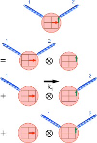
Figure 1: Generation of an unsymmetrized vertex function by convolution.

Gluon actions with relatively short link paths do not require a program for convoluting the rules of individual links; this can easily be done analytically, and Lüscher and Weisz provide an explicit realization of an optimal algorithm in that case. [They also discuss how to automatically generate Feynman rules for gauge-fixing, although for practical purposes this can be done by hand.] In more complex cases however it is advantageous to explicitly code the convolution theorem, applied to basic operators in the action. Consider for instance the NRQCD action

$${\cal L}_{\rm NRQCD}=\psi^{\dagger}\left(1-\frac{a}{2}\delta H\right)\left(1+{\Delta^{(2)}\over 4nM_{0}}\right)^{n}U^{\dagger}_{4}$$

$$\times\left(1+{\Delta^{(2)}\over 4nM_{0}}\right)^{n}\left(1-\frac{a}{2}\delta H\right)\psi-\psi^{\dagger}\psi,$$ (5)

where $\delta H$ has many operators

$$a\delta H\!=\!\!-{c_{3}g\over 8M^{2}}\mbox{{\boldmath$\sigma$}}\cdot({\bf\Delta}\times{\bf E}-{\bf E}\times{\bf\Delta})-{c_{4}g\over 2M}\mbox{{\boldmath$\sigma$}}\cdot{\bf B}+\ldots.$$ (6)

The vertex functions for this extremely complex action can easily be built-up by convolution of the rules for simple operators, such as $\Delta^{(2)}$ and ${\bf E}$ and ${\bf B}$ [6]. We have done a number of calculations for NRQCD using exactly this procedure.

3 Two-loop renormalized coupling

The convergence of perturbative expansions is greatly improved by using a renormalized coupling [10], such as defined by the static-quark potential, according to

$$V(q)\equiv-4\pi C_{F}\alpha_{V}(q)/q^{2}.$$ (7)

We have computed the connection between $\alpha_{V}(q)$ and the bare lattice coupling $\alpha_{0}$ for improved actions in two steps [11]. We first follow Lüscher and Weisz [12], who used a background-field technique to compute the relation between $\alpha_{0}$ and $\alpha_{\overline{\rm MS}}$ for the Wilson gluon action (the matching for Wilson and clover fermions was done in [7]). We then use the relation between $\alpha_{\overline{\rm MS}}$ and $\alpha_{V}$, which is known through third-order [13].

As in the continuum, background-field quantization reduces the number of independent renormalization constants. One computes background- and quantum-field two-point functions on the lattice, $\Gamma^{B}$ and $\Gamma^{A}$ respectively, where

$$\Gamma^{B}(q,-q)^{ab}_{\mu\mu}=-\delta^{ab}3\hat{q}^{2}\left[1-\nu(q)\right]/g_{0}^{2},$$

$$\Gamma^{A}(q,-q)^{ab}_{\mu\mu}=-\delta^{ab}\hat{q}^{2}\left[3\left(1-\omega(q)\right)+\lambda_{0}\right],$$ (8)

where $g_{0}$ and $\lambda_{0}$ are the bare lattice coupling and gauge parameter. Analogous renormalized quantities $g_{\overline{\rm MS}}$, $\nu_{R}$, etc. are defined in the $\overline{\rm MS}$ scheme. The couplings in the two schemes are related by

$$g_{\overline{\rm MS}}^{2}=[1-\nu_{R}(q)]/[1-\nu(q)]\times g_{0}^{2}.$$ (9)

To solve this equation one must account for the implicit dependence on the couplings induced by the relation $\lambda_{R}=[1-\omega_{R}(q)]/[1-\omega(q)]\times\lambda_{0}$.

At two-loop order one must evaluate 31 pure-gauge diagrams, and 18 diagrams with internal fermion lines. In addition one must compute a number of one-loop diagrams that are induced by the $O(g_{0}^{2})$ expansion of the tadpole renormalization factors in the gluon and quark actions.

We evaluate loop integrals by numerical integration using VEGAS. This contrasts with [12, 7], where integrals for unimproved actions were reduced analytically to a small set of primitive integrals. In the present case the much more complex vertices make analytical treatments problematic (see however [14]); moreover there is no gauge in which the improved gluon propagator is diagonal in its Lorentz indices, which further complicates analytical integration. We find that numerical integration gives results of sufficient quality in reasonable computer time. We do integrations at several values of $aq$, and extrapolate to the continuum limit, as illustrated in Fig. 2. We require the fit errors in third-order coefficients to be smaller than the systematic error from the uncalculated fourth-order corrections, for the couplings relevant to simulations.

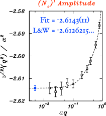
Figure 2: Two-loop results for $\nu(q)$ (Wilson glue).

We also do calculations for several choices of the gauge parameter, to explicitly verify gauge-invariance of the final results. This requires the ${\overline{\rm MS}}$ matching function $\nu_{R}$ at two loops for arbitrary gauge parameter. This was done for the pure-gauge theory by Ellis [15], and we have done the two-loop fermionic part for arbitrary $\lambda_{R}$ (this was previously known only in Feynman gauge [7]).

The relation between the couplings is given by

$$\alpha_{0}=\alpha_{V}(q)\left[1-v_{1}(q)\alpha_{V}(q)-v_{2}(q)\alpha_{V}^{2}(q)\right],$$ (10)

plus corrections of $O(\alpha_{V}^{4})$, where

$$v_{1}(q)=(\beta_{0}/4\pi)\ln(\pi/aq)^{2}+v_{1,0},$$

$$v_{2}(q)=(\beta_{1}/16\pi^{2})\ln(\pi/aq)^{2}-v_{1}^{2}(q^{2})+v_{2,0}.$$ (11)

For the improved actions used by MILC we find

$$v_{1,0}=3.57123(17)-1.196(53)\times 10^{-4}\,N_{f},$$

$$v_{2,0}=5.382(39)-1.0511(51)N_{f}.$$ (12)

4 Wilson loops to third order

One can extract the value of the strong coupling from lattice simulations of short-distance observables. To this end we have evaluated the three-loop PT expansion of Wilson loops [11], extending a clever approach in [7] in order to reduce the number of Feynman diagrams. We evaluate a vacuum-to-vacuum transition amplitude, in the presence of an external “current” generated by the Wilson loop itself

$$\langle W_{R,T}\rangle\Bigl{|}_{S_{\rm lat}}={\partial\over\partial\rho}\langle 1\rangle\Bigl{|}_{S_{\rm lat}+\rho W_{R,T}}\quad\left[\mbox{at\ }\rho=0\right],$$ (13)

using our vertex generators to make the rules for the “extended” action $S_{\rm lat}+\rho W_{R,T}$. This reduces the number of three-loop diagrams by more than half compared to a “direct” evaluation of $\langle W_{R,T}\rangle$.

The third-order expansion has 15 gluonic three-loop diagrams, and 19 fermionic ones. In addition there are a number of one- and two-loop mean-field counterterm diagrams. We quote results for

$$-\!\ln W_{R,T}\!=\!w_{0}\alpha_{\rm V}(q^{*})[1+r_{1}\alpha_{V}+r_{2}\alpha_{V}^{2}]\!+\!\ldots.$$ (14)

The gluonic parts $r_{i,g}$ are given in Table 1, which demonstrates convergence of the renormalized PT expansion through three loops.

Table 1: Perturbative expansions for small Wilson loops for the $O(\alpha_{s}a^{2})$-improved gluon action.

$R$x$T$	$aq^{*}$	$w_{0}$	$r_{1,g}$	$r_{2,g}$
1x1	3.33	3.0684	-0.7753(2)	-0.722(39)
1x2	3.00	5.5512	-0.6202(4)	-0.407(40)
1x3	2.93	7.8765	-0.5335(8)	-0.245(44)
2x2	2.58	9.1998	-0.4934(10)	-0.030(51)

Results for the quenched coupling extracted from simulations at different orders in the perturbative expansion are shown in Fig. 3 [16]. This indicates convergence through fourth order, with the results from two gluon actions at $n$th-order differing by $O(1)\times\alpha_{V}^{n+1}$, all the way from $n=1$ through $n=3$. We are currently analyzing the results for the MILC (2+1)-flavor configurations.

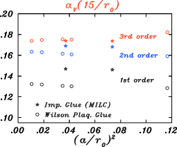
Figure 3: Quenched coupling vs. lattice spacing.

5 Other recent results

The $O(a^{2})$-improved staggered-quark action removes taste-changing interactions at tree level by suppressing the coupling of quarks to high-momentum gluons [1, 2]. The ancient problem of a bad perturbation theory for staggered quarks has also been shown to be thereby eliminated [17]. These effects can be removed at higher orders by introducing four-fermion counterterms, cf. Fig. 4.

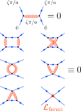
Figure 4: Taste-changing effects for improved-staggered quarks at tree-level and one-loop.

Hasenfratz has found that taste-symmetry breaking can be further reduced by additional smearing and reunitarization of the gauge links in the staggered-quark action [18]. We have found that this improvement is also largely perturbative in origin [19]. Taste-symmetry violations were measured from pion splittings in quenched simulations of staggered actions with different link prescriptions, and calculations of the one-loop four-fermion counterterms were also done in each case. Perturbation theory correctly accounts for changes in the pion splittings with changes in the action, and the same optimal action is found perturbatively and nonperturbatively. Algorithms for doing unquenched simulations with these actions are also under investigation [20].

Another successful PT description of nonperturbative simulation data comes from a computation of the one-loop renormalized anisotropy for improved gluon actions [21]. Perturbative and nonperturbative determinations of the anisotropy were compared over a wide range of lattice spacings and anisotropies, the differences in all cases consistent with an $O(1)\times\alpha_{V}^{2}$ correction.

An important application of lattice PT is matching of the Fermilab and NRQCD heavy-quark actions and associated currents [22, 23, 24, 25]. The first PT matching for the heavy-quark clover interaction was done in [26], and new results were presented here by Kayaba [27]. This is the subject of a concerted effort by the HPQCD collaboration; complete one-loop results for the action parameters are coming soon [23]. We are also well on the road to the two-loop kinetic mass for light and heavy quarks [11] (see also [28]).

6 Monte Carlo methods

There is an attractive alternative to Feynman diagram analysis, which has largely been under-exploited. This is to “do” PT by doing conventional Monte Carlo evaluations of the lattice path integral, but in the “unconventional” weak coupling phase of the theory [29].

One simulates an observable,

$$\langle{\cal O}\rangle=\int[dU_{\mu}(x)][d\bar{\psi}(x)d\psi(x)]\,{\cal O}\,e^{-\beta S_{\rm lat}},$$ (15)

over a range of weak couplings, say $\beta\approx 9\mbox{--}60$, in a finite (Planck!) box, where all lattice momenta are very large (except for possible zero modes, which can be eliminated by an appropriate choice of boundary conditions). One then fits the results to the series $\langle{\cal O}\rangle=\sum_{n}c_{n}\alpha_{V}^{n}(q^{*})$. Third-order expansions of Wilson loops and the static-quark self-energy were obtained in quenched simulations of the plaquette action in [30]. Some results are shown in Fig. 5; the intercept of the graph is the leading order coefficient $c_{0}$, while the slope of the curve resolves $c_{1}$, and its curvature resolves $c_{2}$. We subsequently did the three-loop expansions by Feynman diagrams [11], and the results are in excellent agreement, see Table 2.

Figure 5: Monte Carlo data for a $5\!\times\!5$ Wilson loop, with $\kappa_{1}\!\equiv\!-\ln\langle W_{5\times 5}\rangle/(20\alpha(q^{*}))$ [Wilson glue].

Table 2: Monte Carlo (MC) and PT results for $r_{2,g}$ (Wilson gluon action).

Loop	MC	PT
$1\times 2$	-1.34(8)	-1.31(1)
$1\times 3$	-1.17(9)	-1.13(5)
$1\times 4$	-1.04(9)	-1.00(8)
$1\times 5$	-0.98(11)	-1.05(12)
$2\times 2$	-0.71(8)	-0.71(5)
$2\times 3$	-0.44(9)	-0.48(9)
$3\times 3$	-0.12(9)	0.15(17)

An alternative method has been developed by the Parma group, using an explicit expansion of the Langevin equations in the bare coupling; they have recently obtained the unquenched third-order static-quark self-energy [31]. We have also recently extracted PT expansions from unquenched weak-coupling simulations [32].

7 Summary and outlook

Automatic lattice perturbation theory methods are remarkably simple and powerful. These have been used to do a number of higher-order calculations for highly-improved actions. We have recently done the PT for a third-order determination of $\alpha_{\overline{\rm MS}}(M_{Z})$ from the MILC simulations of (2+1)-flavors of dynamical staggered quarks. Conventional Monte Carlo simulations in the weak-coupling regime may offer a simple alternative to diagrammatic PT, which has so far been under-exploited. Our primary goal is a two-loop determination of heavy-flavor physics. This is an ambitious program but the technology has been proven at the requisite order, and one can reasonably expect that much of this work will be done in the next few years.

I am indebted to Peter Lepage, who has provided much of the rationale for this physics program. I have done most of my PT calculations with Quentin Mason, Matthew Nobes, and Peter Lepage. I have benefited from many discussions with Christine Davies, Junko Shigemitsu, Paul Mackenzie, Andreas Kronfeld, Aida El-Khadra, Richard Woloshyn, and Ron Horgan.

References

- [1] G.P. Lepage, Phys. Rev. D 59, 074502 (1999); Nucl. Phys. Proc. Suppl. 60A, 267 (1998).
- [2] M. Golterman, Nucl. Phys. Proc. Suppl. 73, 906 (1999); J. F. Lagae and D. K. Sinclair, Phys. Rev. D 59, 014511 (1998).
- [3] C. Bernard et al., MILC Collaboration Phys. Rev. D 58, 014503 (1998); 64, 054506 (2001).
- [4] C. T. H. Davies et al., HPQCD Collaboration, hep-lat/0304004.
- [5] M. Lüscher and P. Weisz, Nucl. Phys. B 266, 309 (1986).
- [6] C. Morningstar, Phys.Rev. D 48, 2265 (1993).
- [7] B. Allés et al., Phys. Lett. B 324, 433 (1994); ibid., 426, 361 (1998); C. Christou et al., Nucl. Phys. B 525, 387 (1998); A. Bode and H. Panagopoulos, ibid., 625, 198 (2002).
- [8] S. Capitani and G. Rossi, hep-lat/9504014.
- [9] Q. Mason, Ph. D. thesis, Cornell (2003).
- [10] G. P. Lepage and P. B. Mackenzie, Phys. Rev. D 48, 2250 (1993).
- [11] Q. Mason, H. D. Trottier, and G. P. Lepage, in preparation.
- [12] M. Lüscher and P. Weisz, Nucl. Phys. B 452, 213 (1995); 452, 234 (1995).
- [13] Y. Schröder, Phys. Lett. B 447, 321 (1999).
- [14] T. Becher and K. Melnikov, Phys. Rev. D 66, 074508 (2002); 68, 014506 (2003).
- [15] R. K. Ellis, in Proceedings of the Argonne Workshop on Gauge Theory on a Lattice, eds. C. Zachos et al. (Argonne, 1984). See also [12] and A. van de Ven (1995, unpublished).
- [16] I thank Christine Davies for this data.
- [17] W.-J. Lee and S. R. Sharpe, Phys. Rev. D 66, 114501 (2002), and in these proceedings.
- [18] A. Hasenfratz and F. Knechtli, Phys. Rev. D 64, 034505 (2001); and in these proceedings.
- [19] E. Follana, Q. Mason, C. T. H. Davies, K. Hornbostel, G. P. Lepage, and H. D. Trottier, two talks in these proeceedings.
- [20] K. Hornbostel, G.P. Lepage, R. Woloshyn and K. Wong, private communication.
- [21] I. T. Drummond et al., Phys. Rev. D 66, 094509 (2002).
- [22] A review of heavy-quark physics is given by A. Kronfeld, these proceedings.
- [23] M. Nobes and H. Trottier, these proceedings.
- [24] J. Shigemitsu, E. Gulez and M. Wingate, these proceedings.
- [25] A. Gray, C. Davies and R.R. Horgan, private communication.
- [26] J. Flynn and B. Hill, Phys. Lett. B 264, 173 (1991).
- [27] S. Aoki, Y. Kayaba, and Y. Kuramashi, these proceedings.
- [28] The two-loop additive mass for Wilson quarks was done by E. Follana and H. Panagopoulos, Phys. Rev. D 63, 017501 (2000).
- [29] W.B. Dimm, G.P. Lepage, and P.B. Mackenzie, Nucl. Phys. Proc. Suppl. 42, 403 (1995).
- [30] H. D. Trottier, N.H. Shakespeare, G.P. Lepage and P.B. Mackenzie, Phys. Rev. D 65, 094502 (2002).
- [31] F. Di Renzo, E. Onofri, and G. Marchesini, Nucl. Phys. B 457, 202 (1995); and in these proceedings.
- [32] K. Wong, R. Woloshyn and H.D. Trottier, in preparation.