MS-TP-03-13

DESY 03-156

CERN-TH/2003-233

SFB/CPP-03-45

Non-perturbative Heavy Quark Effective Theory

Jochen Heitger^a and Rainer Sommer^b,c
a Westfälische Wilhelms-Universität Münster, Institut für Theoretische Physik,

Wilhelm-Klemm-Strasse 9, D-48149 Münster, Germany
^b Deutsches Elektronen-Synchrotron DESY, Zeuthen,

Platanenallee 6, D-15738 Zeuthen, Germany
^c CERN, Theory Division, CH-1211 Geneva 23, Switzerland
Abstract

We explain how to perform non-perturbative computations in HQET on the lattice. In particular the problem of the subtraction of power-law divergences is solved by a non-perturbative matching of HQET and QCD. As examples, we present a full calculation of the mass of the b-quark in the combined static and quenched approximation and outline an alternative way to obtain the B-meson decay constant at lowest order. Since no excessively large lattices are required, our strategy can also be applied including dynamical fermions.

Key words: Lattice QCD; Heavy Quark Effective Theory; Static approximation; Non-perturbative renormalization; Matching; Mass of the b-quark; Decay constant

PACS: 11.10.Gh; 11.15.Ha; 12.15.Hh; 12.38.Gc; 12.39.Hg; 14.65.Fy

October 2003

1 Introduction

The physics of the mixing and decays of B-mesons is essential for a determination of unknown CKM-matrix elements and thus for our understanding of the violation of CP-symmetry in Nature. It is also still promising for the discovery of physics beyond the standard model of particle physics. Unfortunately, many of the experimental observations can only be related to the standard model parameters if transition matrix elements of the effective weak Hamiltonian are known. These matrix elements between hadron states are only computable in a fully non-perturbative framework. They provide a strong motivation to study B-physics in lattice QCD. However, as the mass of the b-quark is larger than the affordable inverse lattice spacing in Monte Carlo simulations of lattice QCD, this quark escapes a direct treatment as a relativistic particle. Therefore, effective theories for the b-quark are being developed and used to compute the matrix elements in question [?,?].

The first — and very promising — effective theory that was suggested is the Heavy Quark Effective Theory (HQET) [?,?]. Like others, it is afflicted by a problem which remained unsolved so far: in general its parameters (the coefficients of the terms in the Lagrangian) themselves have to be determined non-perturbatively, as briefly explained in Sect. 2.2. In other words, the theory has to be renormalized non-perturbatively [?]. This fact is simply due to the mixing of operators of different dimensions in the Lagrangian, requiring fine-tuning of their coefficients. If they were determined only perturbatively (in the QCD coupling), the continuum limit of the theory would not exist.

The issue is already present in the determination of the b-quark mass in the static approximation, i.e. in the lowest order of the effective theory. In [?] a strategy was introduced and successfully applied to this problem for the first time, and a general framework for a non-perturbative renormalization of HQET was sketched in [?]. The basic idea, illustrated in Fig. 1, is easily explained.

Figure 1: Relating experimental observables to properly renormalized HQET. $\Gamma_{\rm stat}$ is a renormalized quantity in HQET and $\sigma_{\rm m}(\bar{g}^{2}(L))$ connects $\Gamma_{\rm stat}(L)$ and $\Gamma_{\rm stat}(2L)$; their exact definitions will be given in the course of this paper. In the chosen example, the experimental observable is the mass of the B-meson.

In a finite volume of linear extent $L_{0}={\rm O}(0.2\,{\rm fm})$, one may realize lattices with $am_{{\rm b}}\ll 1$ such that the b-quark can be treated as a standard relativistic fermion. At the same time the energy scale $1/L_{0}={\rm O}(1\,{\rm GeV})$ is still significantly below $m_{{\rm b}}$ and HQET applies quantitatively. Computing the same suitable observables in both theories relates the parameters of HQET to those of QCD. Then one moves, by an iterative procedure that we can still leave unspecified here, to larger and larger volumes and computes HQET observables. This yields the connection to a physically large volume (of linear extent ${\rm O}(2\,{\rm fm})$), where eventually the desired matrix elements are accessible.

Since in this way the parameters of HQET are determined from those of QCD, the predictive power of QCD is transfered to HQET. In addition to solving the renormalization problem of the effective theory, one also eliminates the usual need to determine more and more parameters of the theory from experiment as the effective theory is considered to higher and higher order.

Although related, the strategy we propose here is not to be confused with the one for the computation of the running of the coupling and renormalization group invariant matrix elements as first suggested by Lüscher, Weisz and Wolff [?] and then developed by the ALPHA Collaboration. We will discuss the difference in Sect. 5.2.4.

In this paper we define the effective theory in detail, discussing in particular its renormalization properties (Sect. 2). We then explain the matching between QCD and HQET (Sect. 3) as well as the finite-size strategy (Sect. 4) in the general case. Sect. 5 provides two examples of applications using the effective theory at the lowest order in the inverse b-quark mass. The first one is the computation of the quark mass, where numerical results illustrate that indeed the power-law divergence can be subtracted non-perturbatively, retaining a very good precision for the final physical number. The second one, devoted to the B-meson decay constant, has not yet been applied numerically but is a useful and simple example to help in understanding our method. In Sect. 6 we discuss the potential of our approach as well as the expected uncertainty due to the use of a finite order in the HQET expansion.

2 HQET on the lattice

In this section we define the effective field theory for QCD containing a heavy quark flavour in lattice regularization, starting from the formal $1/m$–expansion of the classical theory. We drop all terms involving the heavy anti-quark fields as they can be incorporated in complete analogy to those containing the heavy quark field $\psi_{\rm h}$ which we discuss in detail. Renormalization properties are addressed but the proper choice of renormalization conditions and the physics content of the theory is deferred to the next section.

2.1 Definition of the effective theory

We consider QCD on the lattice. The explicit form of the gauge field and light fermion action, $S_{\rm rel}$, is not needed for our general discussion, but for some of the following statements to hold, an ${\rm O}(a)$ improved formulation is required, e.g. the one described in [?]. We denote the set of (bare) parameters of the theory with $N_{\rm f}$ relativistic quarks by ${\cal C}_{N_{\rm f}}$. Apart from the gauge coupling, $g_{0}$, and the quark masses, it will in general also cover some improvement coefficients [?].

As has been explained by Eichten and Hill [?,?,?], an effective field theory for hadrons (at rest) containing $N_{\rm f}-1$ light quarks and one heavy quark (b-quark) with mass $m$ may be obtained by a formal $1/m$–expansion of the continuum QCD action and the fields, which appear in the correlation function under study. The action of the heavy quark is written in terms of the four-component field $\psi_{\rm h}$ satisfying

$$P_{+}\psi_{\rm h}=\psi_{\rm h}\,,\quad\overline{\psi}_{\rm h}P_{+}=\overline{\psi}_{\rm h}\,,\quad P_{+}=\hbox{$1\over 2$}(1+\gamma_{0})\,.$$ (2.1)

Including terms up to the order $1/m^{n}$ in the expansion, the action, discretized on a Euclidean lattice, reads

$$S_{\rm HQET} = a^{4}\sum_{x}\Big{\{}{\cal L}_{\rm stat}(x)+\sum_{\nu=1}^{n}{\cal L}^{(\nu)}(x)\Big{\}}\,,$$ (2.2)

$${\cal L}_{\rm stat}(x) = \overline{\psi}_{\rm h}(x)\,[\,\nabla\kern-0.5pt\smash{\raise 4.5pt\hbox{$\ast$}}\kern-4.5pt_{0}+\delta m\,]\,\psi_{\rm h}(x)\,,\qquad$$ (2.3)

$${\cal L}^{(\nu)}(x) = \sum_{i}\omega^{(\nu)}_{i}{\cal L}_{i}^{(\nu)}(x)\,,$$ (2.4)

where $\nabla\kern-0.5pt\smash{\raise 4.5pt\hbox{$\ast$}}\kern-4.5pt_{\mu}$ denotes the backward lattice derivative, $\delta m$ has mass-dimension one, and the local composite fields ${\cal L}_{i}^{(\nu)}$ have mass-dimension $4+\nu$. Indeed, this form is suggested by a formal $1/m$–expansion at the classical level which yields

$$\qquad\delta m =0\,,$$ (2.5)

$${\cal L}_{1}^{(1)} =\overline{\psi}_{\rm h}\Big{(}-{\hbox{$1\over 2$}\,{\bf\sigma}\cdot{\bf B}}\Big{)}\psi_{\rm h}\,, \qquad\omega^{(1)}_{1} =1/m\,,$$ (2.6)

$${\cal L}_{2}^{(1)} =\overline{\psi}_{\rm h}\Big{(}-{\hbox{$1\over 2$}\,{\bf D}^{2}}\Big{)}\psi_{\rm h}\,, \qquad\omega^{(1)}_{2} =1/m$$ (2.7)

up to and including the order $1/m$. Here, ${\bf B}$ is a discretized version of the chromomagnetic field strength and ${\bf D}^{2}$ a lattice version of the covariant Laplacian in three dimensions. Note that a term $m\,\overline{\psi}_{\rm h}(x)\psi_{\rm h}(x)$ has been removed from the action, since it only corresponds to a universal energy shift of all states containing a heavy quark. Removing it makes explicit that the dynamics of heavy-light systems is independent of the scale $m$ at lowest order of $1/m$.

While the action is sufficient to obtain energy levels, for many applications one is interested in (e.g. electroweak transition matrix elements) it becomes necessary to also discuss correlation functions of composite fields. As an example we take the time component of the axial current. In the effective theory it is defined by an expansion similar to eq. (2.2),

$$A^{\rm HQET}_{0}(x) = \sum_{\nu=0}^{n}{\mathcal{A}}^{(\nu)}(x)\,,$$ (2.8)

$${\mathcal{A}}^{(0)}(x) = \alpha^{(0)}_{0}A^{\rm stat}_{0}(x)\,,\quad A^{\rm stat}_{0}(x)=\overline{\psi}_{\rm l}(x)\gamma_{0}\gamma_{5}\psi_{\rm h}(x)\,,$$ (2.9)

$${\mathcal{A}}^{(\nu)}(x) = \sum_{i}\alpha^{(\nu)}_{i}{\mathcal{A}}_{i}^{(\nu)}(x)\,,\quad\nu>0\,,$$ (2.10)

where a light quark field, ${\psi}_{\rm l}$, enters and ${\mathcal{A}}_{i}^{(\nu)}$ is of dimension $3+\nu$. One may then study for instance the correlator (with $(\overline{\psi}_{i}\Gamma\psi_{j})^{\dagger}\equiv\overline{\psi}_{j}\gamma_{0}\Gamma^{\dagger}\gamma_{0}\psi_{i}$)

$$C_{\rm AA}^{\rm HQET}(x_{0})=a^{3}\sum_{{\it\bf x}}\Big{\langle}A^{\rm HQET}_{0}(x)\big{(}A^{\rm HQET}_{0}\big{)}^{\dagger}(0)\Big{\rangle}\,.$$ (2.11)

At the classical level the fields are given by

$$\alpha^{(0)}_{0}=1\,,\quad{\mathcal{A}}_{1}^{(1)}=\overline{\psi}_{\rm l}\gamma_{j}\gamma_{5}\overleftarrow{D}_{j}\psi_{\rm h}\,,\quad\alpha^{(1)}_{1}=1/m\,.$$ (2.12)

In general, i.e. at the quantum level, expectation values are defined by a path integral

$$\langle{\mathcal{O}}\rangle = \hbox{$1\over Z$}\int D[\varphi]\,{\mathcal{O}}[\varphi]\,{\rm e}^{-(S_{\rm rel}+S_{\rm HQET})}\,,$$ (2.13)

$$Z = \int D[\varphi]\,{\rm e}^{-(S_{\rm rel}+S_{\rm HQET})}\,,$$ (2.14)

over all fields with the standard measure, denoted here by $D[\varphi]$. An important ingredient in the definition of the effective field theory is that it is understood throughout that the integrand of the path integral is expanded in a power series in $1/m$, with power counting according to

$$\omega^{(\nu)}_{i}={\rm O}\left(1/m^{\nu}\right)\,,\quad\alpha^{(\nu)}_{i}={\rm O}\left(1/m^{\nu}\right)\,.$$ (2.15)

In other words one replaces

$$\exp\left\{-(S_{\rm rel}+S_{\rm HQET})\right\}=\exp\bigg{\{}-\Big{(}S_{\rm rel}+a^{4}\sum_{x}{\cal L}_{\rm stat}(x)\Big{)}\bigg{\}}\,\times\\ \bigg{\{}1-a^{4}\sum_{x}{\cal L}^{(1)}(x)+\hbox{$1\over 2$}\,\Big{[}\,a^{4}\sum_{x}{\cal L}^{(1)}(x)\,\Big{]}^{2}-a^{4}\sum_{x}{\cal L}^{(2)}(x)+\ldots\bigg{\}}$$ (2.16)

in eq. (2.13). The $1/m$–terms then appear only as insertions of local operators ${\mathcal{O}}_{i}^{(\nu)}(x)$ and ${\mathcal{A}}_{i}^{(\nu)}(x)$ into correlation functions, and the true path integral average is taken with respect to the action in the static approximation for the heavy quark, $S=S_{\rm rel}+a^{4}\sum_{x}{\cal L}_{\rm stat}(x)$.

Power counting leads us to expect that the static theory is renormalizable, requiring a finite number of parameters to be fixed to obtain a continuum limit. Indeed explicit perturbative [?,?,?,?,?] as well as non-perturbative [?] computations support that this is a genuine property of the static effective theory. Would one keep one of the $1/m$–terms in the exponent, as it is done in NRQCD, renormalizability would be lost and most of what we are concluding in this paper would not be true.

We are still left to discuss the renormalization of expectation values of the type (2.13) after inserting the expansion (2.16). This is just the problem of renormalizing correlation functions of local composite operators in the static effective theory. Power counting immediately leads to the conclusion: once all local operators, whose dimensions do not exceed the one of the highest-dimensional operator (i.e. $\nu\leq n$) and which have the proper symmetries, are included, their coefficients may be chosen such that all expectation values have a continuum limit (see e.g. Ref. [?]). Of course, both the operators ${\cal L}_{i}^{(\nu)}(x)$ in the action and the ones in the effective operators such as ${\mathcal{A}}_{i}^{(\nu)}(x)$ have to be included. One may worry that due to the sums over all space-time points in eq. (2.16) contact terms appear, which lead to additional singularities. However, just like in the case of ${\rm O}(a)$ improvement discussed thoroughly in [?], the terms needed to remove these singularities are already present once all local operators with the appropriate dimensions are included.

The effective theory is now defined in terms of the set of parameters,

$${\cal C}_{\rm HQET}\equiv\{c_{k}\}={\cal C}_{N_{\rm f}-1}\cup\{\delta m\}\cup\{\omega^{(\nu)}_{i}\}\cup\{\alpha^{(\nu)}_{j}\}\cup\ldots\,,\quad c_{1}\equiv g_{0}^{2}\,.$$ (2.17)

The ellipses allow for coefficients of further composite operators which will be needed when their correlation functions are considered. For the continuum limit of this effective theory to exist, the parameters $\{c_{k},k>1\}$ have to be chosen properly as a function of $g_{0}^{2}$. Note that in the notation used here, the renormalization of the effective composite fields is included in the set of generalized coupling constants, ${\cal C}_{\rm HQET}$. E.g. at lowest order in $1/m$, the coefficient $\alpha^{(0)}_{0}\equiv Z_{\rm A}^{\rm stat}$ is the renormalization constant of the static axial current [?].

A few more remarks are in order.

• Once the proper degrees of freedom, namely the field $\psi_{\rm h}$, have been identified, the terms in the effective field theory are organized just by their mass-dimension. The expectation that the effective field theory has a continuum limit (is non-perturbatively renormalizable) is thus nothing but the usual expectation that composite operators mix only with operators of the same and lower dimension.

• The same argumentation is also the basis of Symanzik’s discussion of cutoff effects of lattice theories and their removal order by order in $a$ [?,?,?,?]. An important consequence is that in general the $1/m$–expansion and the $a$–expansion are not independent but have to be considered as one expansion in terms of the dimension of the local operators. If we imagine to start with a theory with a set of operators identified by the formal continuum $1/m$–expansion, these operators will for instance mix under renormalization with operators of the same and lower dimension, which are allowed by the lattice symmetries but not by the continuum symmetries and which would therefore not be in the set of the operators one started with. To avoid this, one has to start immediately with the full set of operators of a given dimension, restricted only by the lattice symmetries. In other words we have to count $a={\rm O}(1/m)$. This means also that $S_{\rm rel}$ has to be ${\rm O}(a)$ improved to go to order $1/m$.

• Of course, symmetries restrict the terms that have to be taken into account. In general, out of the space-time symmetries we only have the 3–dimensional cubic group instead of the 4–dimensional hypercubic group. At the lowest order in $1/m$ there are additional symmetries: heavy quark spin-symmetry [?] and the local conservation of heavy quark number, which simplify ${\rm O}(a)$ improvement (see Sect. 2.2 of [?]).

• Furthermore it is convenient to formulate the effective theory only on-shell, i.e. for low energies as well as for correlation functions at physical separations. Then the argumentation of [?] can be taken over literally to show that the equations of motion (derived from the lowest-order action) can be used to reduce the set of operators ${\cal L}_{i}^{(\nu)}(x),{\mathcal{A}}_{i}^{(\nu)}(x),...\,$. Following the same reference, operators obtained by multiplying those of dimension $d$ by a light quark mass are to be counted as separate operators of dimension $d+1$.

• Finally note that after using eq. (2.16), the determinant arising from the static quark action is just an irrelevant constant. In principle, loop effects of the heavy quark are still present in the coefficients $c_{k}$.

2.2 Power divergences and non-perturbative renormalization

The mixing of operators differing in dimensions by $p$ translates into coefficients diverging (when $p>0$) as $a^{-p}$. In the present context it actually has been checked in perturbation theory that these mixings are not forbidden by some accidental symmetry [?]. Due to such power divergences, perturbation theory is not sufficient to determine the coefficients $c_{k}$. An estimate of order $g_{0}^{2l}$ would leave a perturbative remainder

$$\Delta c_{k}\sim g_{0}^{2(l+1)}\,a^{-p}\;\sim\;a^{-p}\,[\ln(a\Lambda)]^{-(l+1)}\;\;\raisebox{-0.43057pt}{ $\stackrel{{\scriptstyle\small{a\to 0}}}{{\longrightarrow}}$}\;\;\;\infty\,\quad$$ (2.18)

with $\Lambda$ the QCD $\Lambda$–parameter. This means that the continuum limit does not exist if the coefficients are determined only perturbatively.

Hence we conclude that a non-perturbative method is needed to determine (at least some of) the parameters $\{c_{k}\}$. Such a method will be introduced in the following two sections.

3 Matching of HQET and QCD

By QCD we denote the theory including a relativistic heavy quark, the b-quark, while with HQET we mean the theory where this quark is incorporated with the action defined in the previous section. The latter is an approximation to QCD when the coefficients ${\cal C}_{\rm HQET}=\{c_{k}\}$ are chosen correctly. Then we expect

$$\Phi^{\rm HQET}(M)=\Phi^{\rm QCD}(M)+{\rm O}\left(1/M^{n+1}\right)$$ (3.19)

for properly chosen observables, $\Phi^{\rm QCD}$, in QCD and their counterparts, $\Phi^{\rm HQET}$, in the effective theory. Amongst the many dependencies of $\Phi^{\rm QCD}$ we have indicated only the one on the heavy quark mass. To be free of any renormalization scheme dependence, we choose the renormalization group invariant (RGI) quark mass denoted by $M$ [?]. In order for eq. (3.19) to hold, all other scales appearing in $\Phi^{\rm QCD}$ are assumed to be small compared to $M$. Choosing as a typical low-energy reference scale of QCD the energy scale $r_{0}^{-1}$($\approx 400\,{\rm MeV}$) [?], defined in terms of the QCD force between static quarks, the combination $r_{0}M$ has to be large. Thus the symbol ${\rm O}(1/M^{n})$ is a short hand for ${\rm O}(1/[r_{0}M]^{n})$.

To give a simple example for a quantity $\Phi^{\rm QCD}$, one could take $\Phi^{\rm QCD}=C_{\rm AA}$, where

$$C_{\rm AA}(x_{0})=Z_{\rm A}^{2}a^{3}\sum_{{\it\bf x}}\Big{\langle}A_{0}(x)(A_{0})^{\dagger}(0)\Big{\rangle}$$ (3.20)

with the heavy-light axial current in QCD, $A_{\mu}=\overline{\psi}_{\rm l}\gamma_{\mu}\gamma_{5}\psi_{\rm b}$, and $Z_{\rm A}$ ensuring the natural normalization of the current consistent with current algebra [?,?]. Then eq. (3.19) is valid for $\Phi^{\rm HQET}={\rm e}^{-mx_{0}}C_{\rm AA}^{\rm HQET}(x_{0})$ with $C_{\rm AA}^{\rm HQET}(x_{0})$ from eq. (2.11) and in the region $1/x_{0}\ll M$. With the latter, kinematical, condition one takes care that the correlation functions are dominated by states with energies (the heavy quark mass being subtracted) small compared to $M$. Furthermore, the factor ${\rm e}^{-mx_{0}}$ accounts for the mass term that had been removed from the effective theory Lagrangian as already mentioned after eq. (2.2). Which mass $m$ is to be taken here, depends on the convention used to define $\delta m$. As will be explained further in Sect. 5.1.1, at each order in $1/m$, the combination $m+\hbox{$1\over a$}\ln(1+a\delta m)$ is uniquely fixed by the matching of HQET and QCD. We emphasize again that the same mass $m$ enters all correlation functions involving one heavy quark.

Let us now come to the main problem: determining the parameters in the effective theory such that this equivalence between HQET and QCD is true. First of all assume that the parameters of QCD have been fixed by requiring a set of observables, e.g. a set of hadron masses, to agree with experiment. It is then sufficient to impose

$$\Phi^{\rm HQET}_{k}(M)=\Phi^{\rm QCD}_{k}(M)\,,\quad k=1,\ldots,N_{n}\,,$$ (3.21)

to determine all parameters $\{c_{k}\,,k=1,\ldots,N_{n}\}$ in the effective theory. Observables used originally to fix the parameters of QCD may be amongst these $\Phi^{\rm QCD}_{k}$. The matching conditions, eq. (3.21), define the set $\{c_{k}\}$ for any value of the lattice spacing (precisely speaking, for any value of $a/r_{0}$).

In principle, each $\Phi^{\rm HQET}_{k}$ could be determined from a physical, experimentally accessible observable. However, this would reduce the predictive power of the effective theory since it contains more parameters than QCD. Particularly for increasing the order $n$ of the $1/m$–expansion we then would need to use more and more experimental observables.

To preserve the predictability of the theory, we may instead insert some quantities $\Phi^{\rm QCD}_{k}(M)$ computed in the continuum limit of lattice QCD. This of course demands to treat the heavy quark as a relativistic particle on the lattice, seemingly in contradiction to the very reason to consider the effective theory: small enough lattice spacings to do this are very difficult to reach. An additional ingredient is thus necessary to make the idea practicable. It will be explained in the following section. At this stage the important point is that there are no theoretical obstacles to a non-perturbative matching. We end this section with some comments on details of the general matching procedure.

• The observables $\Phi$ are assumed to be renormalized. Eq. (3.21) is, however, used to fix the bare parameters in the action — for each value of $g_{0}^{2}$.

• When one increases the order $n$ in the expansion, new quantities $\Phi_{k}$ have to be added, and at the same time, the parameters of the lower-order Lagrangian, $c_{i}$, $i\leq N_{n-1}$, will change in general. This change is due to mixing of the operators and may thus be sizeable.

• It is convenient to take the continuum limit of $\Phi^{\rm QCD}_{k}$ before imposing eq. (3.21). If one decides not to do this, the lattice spacings on both sides of eq. (3.21) should be scaled together in order to reach the continuum limit in the effective theory.

• As mentioned already in the previous section, the terms necessary for Symanzik improvement are taken into account automatically, namely some of the equations (3.21) may be interpreted as improvement conditions. Working up to the order $n$, the resulting lattice HQET is correct up to

  $$\text{error terms}={\rm O}\left((1/m)^{n+1}\right)={\rm O}\left(M^{-(n+1)}(aM)^{k}\right)\,,\quad k=0,1,\ldots,n+1\,.$$ (3.22)

  Higher-order terms in $1/M$ have parametrically larger lattice spacing errors. For example, a treatment of the theory including the next-to-leading operators will give us the $(1/M)^{0}$–terms with ${\rm O}(a^{2})$ errors and the linear $1/M$–corrections with ${\rm O}(a)$ uncertainties. Additional work would be necessary to suppress the discretization effects in the $1/M$–terms to ${\rm O}(a^{2})$.

• There is a close analogy of our proposed matching procedure to what is done when the low-energy constants of the chiral effective Lagrangian [?] are determined using lattice QCD. An important difference is, however, that the chiral expansion can be worked out analytically while here we still have to evaluate the resulting theory by Monte Carlo. The reason is that strong interactions remain; the lowest-order theory, the static approximation, is non-trivial.

4 The rôle of finite volume

From the theoretical point of view, the matching described in the previous section is sufficient. However, we should take into consideration what can be done in a numerical computation. To give a concrete example, let us assume that

$$(L/a)^{3}\times T/a\leq 32^{3}\times 64$$ (4.23)

lattices can be simulated, numbers which are realistic for present computations in the quenched approximation, but too large for full QCD. We further assume that we deal with quantities which have negligible finite size effects when

$$L\geq 2\,{\rm fm}\,.$$ (4.24)

Then the smallest lattice spacing reachable is $a\approx 0.06\,{\rm fm}$, and this number will not be very different if the above assumptions are modified within reasonable limits. While such a lattice spacing is small enough to perform computations for charm quarks [?,?], the subtracted bare mass of the b-quark is about $am_{\rm q}\approx 1$. In this situation lattice artifacts are expected to be very large and it is impossible to obtain the r.h.s. of eq. (3.21).

The situation becomes quite different when one considers observables $\Phi_{k}$ defined in finite volume with $L$ considerably smaller than $2\,{\rm fm}$ and uses the generally accepted — and also much tested — assumption that both QCD and HQET are applicable in a finite volume and the parameters in the Lagrangians are independent of the volume.

4.1 Matching in finite volume

Instead of eq. (3.21) we now consider (remember that $N_{n}$ is the number of parameters in the effective theory):

$$\Phi^{\rm HQET}_{k}(L,M)=\Phi^{\rm QCD}_{k}(L,M)\,,\quad k=1,\ldots,N_{n}\,.$$ (4.25)

This will allow us to have much smaller lattice spacings on the r.h.s. in order to eventually approach the continuum limit. A typical choice is $L=L_{0}\approx 0.2\,{\rm fm}$. As has been shown in the preliminary report of our work [?], eq. (4.25) can be evaluated very precisely for suitably selected quantities $\Phi^{\rm QCD}_{k}$ and the continuum limit can actually be taken.

Concerning the l.h.s., we have to take into account that $a$–effects will certainly be significant when the resolution $a/L$ of the finite space-time is too coarse. Hence the lattice spacings where the bare parameters $\{c_{k}(g_{0})\}$ can be determined are $a={\rm O}(0.02\,{\rm fm})={\rm O}(L_{0}/10)$. For such values of $a$, the computation of the physical observables in the infinite-volume theory ($L\approx 2\,{\rm fm}$ in practice) would again be impracticable, because lattices with too many points $(L/a)^{4}$ would be required. Therefore, a further step is necessary to make larger lattice spacings and thereby larger physical volumes available in the effective theory.

4.2 Finite-size scaling

Also for this step a well-defined procedure is easily found. First assume that all observables $\Phi^{\rm HQET}_{k}(L,M)$ have been made dimensionless by multiplication with appropriate powers of $L$. Next we define step scaling functions [?], $F_{k}$, by

$$\Phi^{\rm HQET}_{k}(sL,M)=F_{k}\left(\big{\{}\Phi^{\rm HQET}_{j}(L,M)\,,\,j=1,\ldots,N_{n}\big{\}}\right)\,,\quad k=1,\ldots,N_{n}\,,$$ (4.26)

where typically one uses scale changes of $s=2$. These dimensionless functions describe the change of the complete set of observables $\{\Phi^{\rm HQET}_{k}\}$ under a scaling of $L\to sL$, and we briefly sketch how they can be computed. One selects a lattice with a certain resolution $a/L$. The specification of $\Phi^{\rm HQET}_{j}(L,M)$, $j=1,\ldots,N_{n}$, then fixes all (bare) parameters of the theory. The l.h.s. of eq. (4.26) is now computed, keeping the bare parameters fixed while changing $L/a\to L^{\prime}/a=sL/a$. Repeating this for a few values of $a/L$, the continuum limit of $F_{k}$ can be obtained by an extrapolation $a/L\rightarrow 0$.

An important practical detail is to choose the various quantities $\Phi^{\rm HQET}_{k}$ such that each $F_{k}$ depends only on a few $\Phi^{\rm HQET}_{j}$ and the bare parameters $c_{k}$ can be determined rather independently from each other. For instance, it is natural to identify the running Schrödinger functional coupling $\bar{g}^{2}(L)$ [?,?] with $\Phi^{\rm HQET}_{1}(L,M)$ and to keep all of the light quark masses zero in these steps. In this way $g_{0}^{2}$ and the (light) bare quark masses are fixed independently of the parameters $\delta m,\omega^{(\nu)}_{i},\alpha^{(\nu)}_{i},\ldots$ coming from the heavy sector. In the quenched approximation or with two dynamical quarks, the set of bare parameters specifying the relativistic sector, ${\cal C}_{N_{\rm f}-1}$, can then be taken over from [?,?,?,?] without change.

A few steps — may be two — are necessary to reach a value of $L={\rm O}(1\,{\rm fm})$, where at the same time contact can be made with resolutions $a/L$ that are affordable to accommodate the suitable observables on a physically large lattice to realize the original matching condition, eq. (3.21). (In our first example, Sect. 5.1, this rôle will be played by the B-meson with its mass as the physical input.) We note that in principle the size of $L_{0}$ is rather arbitrary, but the following consideration is important. We are matching at a finite value of $1/m$ and a finite order $n$. Thus the final results will depend on which quantities have been used to perform the matching. If one chooses quantities with kinematics where the $1/m$–expansion is not accurate (or even not applicable), this will translate into badly determined parameters in the effective Lagrangian and large final truncation errors. For this reason, $L_{0}$ has to be chosen such that the $1/m$–expansion is applicable which means

$$1/L_{0}\ll m\,,$$ (4.27)

and $L_{0}$ cannot be too small. From these considerations it appears that $L_{0}\approx 0.2\,{\rm fm}\,-\,0.4\,{\rm fm}$ is a good choice.

4.3 Evaluation of the physical observables in the effective theory

Physical observables usually have to be computed in large volume which, for practical reasons, means at lattice spacings around $1/20\,{\rm fm}$ to $1/10\,{\rm fm}$. In this region the bare parameters of the effective theory are determined as follows.

One chooses a suitable $K$ such that

$$L_{K}=s^{K}L_{0}\approx 1\,{\rm fm}\,.$$ (4.28)

Iterated applications of eq. (4.26) give rise to recursion relations, the solutions of which determine quantities $V_{k}\equiv\Phi^{\rm HQET}_{k}(L_{K},M)$ in the larger volume of extent $L_{K}$. Next, regarding $\Phi^{\rm HQET}_{k}(L_{K},M)=V_{k}$ as a requirement while setting the number of lattice points to $L_{K}/a={\rm O}(10)$ just fixes the bare parameters ${\cal C}_{\rm HQET}$. These bare parameters are then known at values of the lattice spacing, where the computation of correlation functions in large volume is possible in the effective theory and masses and matrix elements can be extracted from their large-time behaviour.

Note that in the notation used here also the renormalization constants of the composite operators appearing in the correlation functions are amongst the “bare parameters”. All quantities are thus renormalized entirely non-perturbatively. One may still wonder how $M$ itself is fixed. The answer to this question is provided by the first of the two examples, which we will use now to illustrate the general strategy.

5 Examples

In this section we supply two applications of our non-perturbative matching strategy of HQET and QCD that up to now was formulated in rather general terms: a full calculation of the b-quark mass in combined static and quenched approximations (Sect. 5.1) and a proposal for a non-perturbative determination of multiplicatively renormalized matrix elements of the static-light axial current, which is different in spirit from Ref. [?] and still awaits a numerical investigation.

5.1 The b-quark mass at lowest order

Several determinations of the mass of the b-quark, which use the static approximation on the lattice (HQET to order $(1/m)^{0}$), have been published [?]. They all rely on a perturbative estimate of $\delta m$ [?,?,?] and suffer from a power-law divergence due to the mixing of $\overline{\psi}_{\rm h}D_{0}\psi_{\rm h}$ and $\overline{\psi}_{\rm h}\psi_{\rm h}$ as discussed in Sect. 2.2. Their precision is thus limited by the fact that a continuum limit can not be taken, and it is difficult to estimate the associated uncertainty. We here explain how a entirely non-perturbative computation can be done and will also give a first result, which can easily be improved in precision in the near future. This step is also a prerequisite to perform the matching of other quantities such as the axial current, since generically the quark mass enters in the matching step (4.25) for all $\Phi_{k}$.

5.1.1 Strategy and basic formula

As indicated already in Sect. 4, given a resolution $a/L$, we fix $g_{0}^{2}$ such that the finite-volume running coupling of Ref. [?] takes a certain value. Furthermore we set the light quark masses to zero (with one exception which will be discussed). In the language of Sect. 4 we have

$$\Phi^{\rm HQET}_{1} = \bar{g}^{2}(L)\,,$$ (5.29)

$$\Phi^{\rm HQET}_{k+1} = m^{\rm PCAC}_{k}\,\,\,=\,\,\,0\,,\quad k=1,\ldots,N_{\rm f}-1\,,$$ (5.30)

in terms of the PCAC masses of the light flavour number $k$, $m^{\rm PCAC}_{k}$, and the running coupling $\bar{g}^{2}(L)$ in the Schrödinger functional (SF) scheme [?]. Other choices are possible, but the above is convenient in view of the present numerical knowledge [?,?,?]. The box length $L$ is then parametrized through $\bar{g}^{2}(L)$. A very useful feature of eqs. (5.29) and (5.30) is that they do not involve the heavy field at all and determine the bare coupling and quark masses independently of the heavy sector; in particular these conditions are independent of the order $n$ of the expansion.

In this section we are only concerned with energies and remain at lowest order in $1/m$. The only additional parameter in the Lagrangian to be fixed is $a\delta m$, i.e. one more condition corresponding to $k=N_{\rm f}+1$ in eq. (4.25) is needed. We start from a time-slice correlation function projected onto spatial momentum zero containing one heavy quark (such as $C_{\rm AA}$, eq. (3.20)). Denoting it generically as $C(x_{0})$, in the logarithmic derivative

$$\Gamma=\hbox{$1\over 2a$}\ln\Big{[}\,C(x_{0}-a)/C(x_{0}+a)\,\Big{]}\qquad\left(\mbox{$x_{0}/L$ fixed}\right)$$ (5.31)

all multiplicative renormalization factors of $C(x_{0})$ cancel. Below we shall use $x_{0}/L=1/2$, but other choices are possible. Replacing the fields in the correlation function $C(x_{0})$ by the corresponding effective fields defines $C^{\rm HQET}(x_{0})$ in the effective theory. In the static approximation, its logarithmic derivative, $\Gamma_{\rm stat}$, built as in eq. (5.31), depends on $\delta m$ in the simple form

$$\Gamma_{\rm stat}=\left.\Gamma_{\rm stat}\right|_{\delta m=0}+\hbox{$1\over a$}\ln(1+a\delta m)\,,$$ (5.32)

as is easily seen from the explicit form of the static quark propagator. In large volume, which due to $x_{0}/L=\mbox{constant}$ also means large Euclidean time, $\Gamma=\Gamma(L,M)$ will turn into the mass of a b-hadron, say $m_{\rm B}$. It is now obvious that

$$\Phi^{\rm QCD}_{N_{\rm f}+1}(L,M) \equiv L\,\Gamma\,,\quad$$ (5.33)

$$\Phi^{\rm HQET}_{N_{\rm f}+1}(L,M) \equiv L\,(\Gamma_{\rm stat}+m)$$

$$= L\left(\left.\Gamma_{\rm stat}\right|_{\delta m=0}+m_{\rm bare}\right)\,,\quad m_{\rm bare}=m+\hbox{$1\over a$}\ln(1+a\delta m)\,,$$

are sensible assignments to fix the combination $m_{\rm bare}$ via requiring

$$\Phi^{\rm QCD}_{N_{\rm f}+1}(L,M)=\Phi^{\rm HQET}_{N_{\rm f}+1}(L,M)\,.$$ (5.35)

Since $\delta m$ and $m$ always appear in the combination $m_{\rm bare}$, they may not be fixed separately, unless one arbitrarily defines $\delta m$ by an additional condition.

Due to eq. (5.32), the step scaling function

$$\sigma_{\rm m}\left(\bar{g}^{2}(L)\right)\equiv 2L\,[\,\Gamma_{\rm stat}(2L,M)-\Gamma_{\rm stat}(L,M)\,]$$ (5.36)

is independent of $m_{\rm bare}$ and therefore also independent of $M$; at lowest order in $1/m$, energy differences in the effective theory do not depend on the heavy quark mass. The step scaling function (5.36) is thus a particularly simple realization of eq. (4.26). Together with the one for the running coupling [?,?],

$$\sigma(u)=\left.\bar{g}^{2}(2L)\right|_{\bar{g}^{2}(L)=u}\,,$$ (5.37)

it defines the sequence

$$u_{0}=\bar{g}^{2}(L_{0})\,, w_{0}=\left.L\,\Gamma_{\rm stat}\right|_{L=L_{0}}\,,$$ (5.38)

$$u_{k+1}=\sigma(u_{k})\,, w_{k+1}=2w_{k}+\sigma_{\rm m}(u_{k})\,,$$ (5.39)

which is easily seen to relate $\Gamma_{\rm stat}(L_{K},M)$, with $L_{K}=2^{K}L_{0}$, to $\Gamma_{\rm stat}(L_{0},M)$ when the sequence $u_{0},\ldots,u_{K-1}$ is known:

$$L_{0}\Gamma_{\rm stat}(L_{K},M)=L_{0}\Gamma_{\rm stat}(L_{0},M)+\sum_{k=0}^{K-1}2^{-(k+1)}\sigma_{\rm m}(u_{k})\,.$$ (5.40)

Suitable choices for $u_{0}$ and $K$ then allow to arrive at $L_{K}={\rm O}(1\,{\rm fm})$.

Finally one considers the energy $E_{\rm stat}$ of a B-meson in static approximation, given for example by

$$C_{\rm AA}^{\rm HQET}(x_{0})\,\raisebox{-0.43057pt}{ $\stackrel{{\scriptstyle\small{x_{0}\to\infty}}}{{\sim}}$}\,A\exp(-x_{0}E_{\rm stat})\qquad\left(\mbox{$L$ large}\right)\,.$$ (5.41)

The energy difference

$$\Delta E=E_{\rm stat}-\Gamma_{\rm stat}(L_{K},M)$$ (5.42)

can be computed with one and the same lattice spacing (i.e. at the same bare parameters) for the two different terms on the r.h.s., but of course with different $L$. Combining eq. (5.35) imposed in small volume ($L=L_{0}$) with eqs. (5.40) and (5.42) to eliminate $m_{\rm bare}$ in $m_{\rm B}=E_{\rm stat}+m_{\rm bare}$ (holding in the large-volume limit), we arrive at the basic equation

$$L_{0}m_{\rm B}=L_{0}\Gamma(L_{0},M_{{\rm b}})+\sum_{k=0}^{K-1}2^{-(k+1)}\sigma_{\rm m}(u_{k})+L_{0}\Delta E\,.$$ (5.43)

It relates the mass of the B-meson to a quantity $\Gamma(L_{0},M_{{\rm b}})$, computable in lattice QCD with a relativistic b-quark, and the energy differences $\Delta E$ and $\sigma_{\rm m}$ which are both defined and computable in the effective theory. All quantities on the r.h.s. may be evaluated in the continuum limit. Note that all of the terms in eq. (5.43) are independent of $m_{\rm bare}$ (because the unknown $m_{\rm bare}$, and thereby $\delta m$ too, drop out in the differences), although logically eq. (5.35) has been used to fix it non-perturbatively. Our strategy has also been presented in a somewhat different way, which is closer in spirit and notation to standard HQET applications (but less rigorous), in [?].

Eq. (5.43) may be looked at in two different ways. Given the RGI mass of the b-quark, $M_{{\rm b}}$, eq. (5.43) provides a way to compute the mass of the B-meson. It is more interesting to turn this around: taking $m_{\rm B}$ from experiment and evaluating (in lattice QCD) $\Gamma(L_{0},M)$ as a function of $M$, this equation may be solved for $M_{{\rm b}}$. Implicitly the bare parameter $m_{\rm bare}$ is thus fixed non-perturbatively, and the problem of a power-law divergence is solved.

We now give an example for a precise definition of the correlation function $C(x_{0})$ and use the quenched approximation to demonstrate that the continuum limit can be reached in all steps while still a very interesting precision is attainable. The reader who is not interested in the numerical details may directly continue with Sect. 5.2.

5.1.2 Correlation functions, ${\rm O}(a)$ improvement and spin-symmetry

In our numerical implementation we choose SF boundary conditions with all details as in [?], including $\theta=1/2$, $T=L$ and $C=C^{\prime}=0$ in the notation of that paper. This means that ${\rm O}(a)$ improvement [?,?] is fully implemented, except for uncertainties in the coefficients $c_{\rm A}^{\rm stat}$, $c_{\rm t}$ and $\widetilde{c}_{\rm t}$ originating from their only perturbative estimation. As in [?] it has been checked that the influence of these uncertainties on the observables considered here can be neglected compared to our statistical errors. We will therefore not mention ${\rm O}(a)$ terms any more and perform continuum extrapolations modelling the $a$–effects as ${\rm O}(a^{2})$.

For our definition of $\Gamma$ we consider the two correlation functions

$$f_{\rm A}(x_{0}) = -{a^{6}\over 2}\sum_{{\it\bf y},{\it\bf z}}\,\left\langle(A_{{\rm I}})_{0}(x)\,\overline{\zeta}_{\rm b}({\it\bf y})\gamma_{5}\zeta_{\rm l}({\it\bf z})\right\rangle\,,$$ (5.44)

$$k_{\rm V}(x_{0}) = -{a^{6}\over 6}\sum_{{\it\bf y},{\it\bf z},k}\,\left\langle(V_{{\rm I}})_{k}(x)\,\overline{\zeta}_{\rm b}({\it\bf y})\gamma_{k}\zeta_{\rm l}({\it\bf z})\right\rangle\,,$$ (5.45)

where the label “$\rm I$” on the axial and vector currents reminds us that their ${\rm O}(a)$ improved forms are used:

$$(A_{{\rm I}})_{\mu}(x) = \overline{\psi}_{\rm l}(x)\gamma_{\mu}\gamma_{5}\psi_{\rm b}(x)+ac_{\rm A}{\textstyle{\hbox{$1\over 2$}}}({\partial_{\mu}}+\partial\kern-0.5pt\smash{\raise 4.5pt\hbox{$\ast$}}\kern-5.0pt_{\mu})\left\{\overline{\psi}_{\rm l}(x)\gamma_{5}\psi_{\rm b}(x)\right\}\,,$$ (5.46)

$$(V_{{\rm I}})_{\mu}(x) = \overline{\psi}_{\rm l}(x)\gamma_{\mu}\psi_{\rm b}(x)+ac_{\rm V}{\textstyle{\hbox{$1\over 2$}}}({\partial_{\nu}}+\partial\kern-0.5pt\smash{\raise 4.5pt\hbox{$\ast$}}\kern-5.0pt_{\nu})\left\{i\,\overline{\psi}_{\rm l}(x)\sigma_{\mu\nu}\psi_{\rm b}(x)\right\}\,.$$ (5.47)

As a consequence of the heavy quark spin-symmetry, their partners in the effective theory coincide exactly at lowest order in $1/m$ and we thus define only one

$$C^{\rm HQET}(x_{0})\equiv f_{\rm A}^{\rm stat}(x_{0})=-{a^{6}\over 2}\sum_{{\it\bf y},{\it\bf z}}\,\left\langle(A^{\rm stat}_{\rm I})_{0}(x)\,\overline{\zeta}_{\rm h}({\it\bf y})\gamma_{5}\zeta_{\rm l}({\it\bf z})\right\rangle\,.$$ (5.48)

In these definitions, $\sum_{{\it\bf y},{\it\bf z}}\overline{\zeta}_{\rm b}({\it\bf y})\gamma_{5}\zeta_{\rm l}({\it\bf z})$ and $\sum_{{\it\bf y},{\it\bf z}}\overline{\zeta}_{\rm h}({\it\bf y})\gamma_{5}\zeta_{\rm l}({\it\bf z})$ are interpolating fields localized at the $x_{0}=0$ boundary of the SF, which create a state with the quantum numbers of a B-meson with momentum ${\bf p}={\bf 0}$, and for $\gamma_{5}\to\gamma_{k}$ we have the quantum numbers of a B^∗. The correlation functions are schematically depicted in Fig. 2; more details can be found in [?].

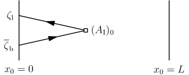
Figure 2: Illustration of the correlation function $f_{\rm A}$. For $k_{\rm V}$, the insertion of $(A_{{\rm I}})_{0}$ is replaced by $(V_{{\rm I}})_{k}$, whereas in case of $f_{\rm A}^{\rm stat}$ the operator in the bulk is $(A^{\rm stat}_{\rm I})_{0}$ connected to $\overline{\zeta}_{\rm h}$ (instead of $\overline{\zeta}_{\rm b}$) by a static quark propagator.

Inserting $C(x_{0})=f_{\rm A}(x_{0})$ and $C(x_{0})=k_{\rm V}(x_{0})$ into eq. (5.31) defines $\Gamma_{\rm PS}$ and $\Gamma_{\rm V}$, respectively. Their partner in the effective theory is denoted as $\Gamma_{\rm stat}$. Due to the spin-symmetry, either $L\Gamma_{\rm PS}=L(\Gamma_{\rm stat}+m)$ or $L\Gamma_{\rm V}=L(\Gamma_{\rm stat}+m)$ are possible matching conditions at lowest order in $1/m$. At first order, one has to consider also separately the vector and the axial vector correlators in the effective theory since these are split by the $\sigma\cdot{\bf B}$–term in the effective Lagrangian. It is then convenient to define the matching condition as eq. (5.35) with the spin-average

$$\Gamma=\hbox{$1\over 4$}\left(\Gamma_{\rm PS}+3\Gamma_{\rm V}\right)\,.$$ (5.49)

With this definition the matching condition (5.35) is independent of the coefficient of the $\sigma\cdot{\bf B}$–term also at first order in $1/m$, and hopefully $1/m$–effects are thereby minimized.

Having now completed our definition of $\Gamma$ and $\Gamma_{\rm stat}$, we remind the reader that the mass of the light quark is set to zero and thus $\Gamma$ is only a function of the heavy quark mass, $M$, and the linear extent of the SF-volume, $L$ (if $a$–effects are neglected for the moment).

5.1.3 Matching

The essential steps of our strategy explained in Sect. 5.1.1 are the matching at $L=L_{0}$ as the starting point, then connecting to $L=L_{K}$ and from there to the (infinite-volume) meson mass. In practice, proceeding from any choice of $u_{0}$ the sequence $u_{k}$ is only known with a certain numerical precision and this has to be taken into account in the error analysis. Furthermore we want to take advantage of the numerical results of [?] for triples of $(L/a,\beta,\kappa)$ corresponding to fixed renormalized coupling and vanishing light quark mass in the quenched approximation, as well as of the known function $[r_{0}/a](\beta)$ and the value of $L_{\rm max}/r_{0}=0.718(16)$ [?], where $\bar{g}^{2}(L_{\rm max})=3.48$. So it is convenient to have $K=2$ in previous formulae and to define (exactly) $L_{2}=2L_{\rm max}=1.436\,r_{0}$. Then, applying the inverse of the step scaling function of the coupling [?] twice, we arrive at

$$u_{0}=2.455(28)\,,\quad\sigma^{-1}(u_{0})=1.918(20)\,,$$ (5.50)

and end up with $L=L_{0}=L_{2}/4=0.359\,r_{0}\approx 0.18\,{\rm fm}$ for the linear extent of the matching volume. The matching of HQET and QCD is then supposed to be done at $u=u_{0}\approx 2.4$. We could thus keep e.g. $u=2.4484$ fixed, where the triples $(L/a,\beta,\kappa)$ are known [?], but only for $6\leq L/a\leq 16$. The spacing of these lattices is still too large to comfortably accommodate a propagating b-quark. Instead it is better to work at a constant value of $u=1.8811$, varying $6\leq L/(2a)\leq 16$. Nevertheless, $\Gamma$ is computed on the lattices with $L/a$ points per direction, and the slight mismatch of $\sigma^{-1}(u_{0})$ and $1.8811$ will eventually be taken into account together with the overall error analysis.

We now have to determine $\Gamma(L,M)$, where in case of the relativistic theory $L$ is always to be identified with the extent of the matching volume, $L_{0}$, from now on. In order to approach its continuum limit, we define

$$\Omega(u,z,a/L)=\left.L\,\Gamma(L,M)\right|_{\bar{g}^{2}(L/2)=u\,,\,LM=z}$$ (5.51)

and extrapolate it as a function of $a/L$, viz.

$$\omega(u,z)=\lim_{a/L\to 0}\Omega(u,z,a/L)\,,$$ (5.52)

for a few selected values of $z$ and at fixed $u$. This requires to compute $\Omega$ with $z$ and $u$ fixed while changing $L/a$ and therefore also $\beta$. A particular aspect in this step is that in imposing the condition of fixed $z$ (at variable $\beta$), the relation between the bare quark mass, $m_{\rm q}$, and the RGI one, $M$, is needed, where several renormalization factors and improvement coefficients enter. Although they had already been determined [?,?], it turned out that it was desirable to improve their precision and to determine them directly in the range of $\beta$ where they are needed in the present application. For this reason they were redetermined in Ref. [?], and also $\omega$ as a function of $z$, eq. (5.52), was obtained by extrapolation in $a/L\to 0$ in that work. For the reader’s convenience, we reproduce from [?] a graph of the continuum values $\omega(1.8811,z)$ together with the fit function

$$\omega(1.8811,z)=a_{0}z+a_{1}+a_{2}\,\hbox{$1\over z$}\,,\quad a_{0}=0.581\,,\quad a_{1}=1.226\,,\quad a_{2}=-0.358$$ (5.53)

in Fig. 3.

Figure 3: Continuum limit values of $L_{0}\Gamma(L_{0},M)$ at fixed coupling $\bar{g}^{2}(L_{0}/2)=1.8811$ as a function of $z=L_{0}M$ and its fit function, determined in relativistic QCD but small volume [?]. The b-quark mass scale lies near $z\approx 6$.

In the interval $5.2\leq z\leq 6.6$, which is the relevant $z$–range to extract the RGI b-quark mass later, this parametrization describes $\omega(1.8811,z)$ with a precision of about 0.5%. A further global uncertainty of 0.9% has to be attributed to the argument $z$ of the function $\omega$ (see Ref. [?]). In order to also take the small statistical error and mismatch in $u_{0}$ into consideration at the end, we also need a numerical value for the derivative of $\omega^{\prime}(1.8811,z)$ w.r.t. $u$. It was found to be constant in the interesting region [?]:

$$\left.{\partial\over\partial u}\,\omega(u,z)\right|_{u=1.8811}=0.70(1)\,,\quad 6.0\leq z\leq 6.6\,.$$ (5.54)

For completeness we also quote the fit result for $\omega(1.8811,z)$, if instead of the spin-average (5.49) it is defined as the continuum limit of the effective energy $L\Gamma_{\rm PS}(L,M)$. With the same fit ansatz as in eq. (5.53), the coefficients then read

$$a_{0}=0.587\,,\quad a_{1}=1.121\,,\quad a_{2}=-1.306\qquad\left(\mbox{for $\Gamma\equiv\Gamma_{\rm PS}$}\right)\,.$$ (5.55)

The significantly larger $a_{2}$–term in this case compared to eq. (5.53) indicates that the spin-averaged combination $\Gamma$ has smaller $1/m$–errors and should therefore be preferred in the implementation of the matching step.

5.1.4 Finite-size scaling

The next step is the numerical determination of the step scaling function $\sigma_{\rm m}$, eq. (5.36), and then of the ($M$–independent difference) $L_{0}[\Gamma_{\rm stat}(L_{K},M)-\Gamma_{\rm stat}(L_{0},M)]$ as given by eq. (5.40).

Figure 4: Lattice step scaling function $\Sigma_{\rm m}$ and its continuum limit extrapolation linear in $(a/L)^{2}$, which uses only the four smallest values of $a/L$.

$u$			$\sigma_{\rm m}(u)$
2.4484			$-0$.	$205(18)$
2.7700			$-0$.	$133(26)$
3.4800			$0$.	$040(25)$

Table 1: Results for the continuum step scaling function $\sigma_{\rm m}(u)$.

At finite lattice spacing, the step scaling function is defined by

$$\Sigma_{\rm m}(u,a/L)=\left.2L\,[\,\Gamma_{\rm stat}(2L,M)-\Gamma_{\rm stat}(L,M)\,]\right|_{\bar{g}^{2}(L)=u}\,,$$ (5.56)

where, as mentioned earlier, the (light) quark mass is set to zero. The exact definition of the massless point does not play an important rôle; it is as in Ref. [?]. In fact, we evaluated $\Sigma_{\rm m}$ directly from the correlation functions computed there, where details of the simulations can be found, too. Numerical results for $\Sigma_{\rm m}$ are listed in Table A.1 in the appendix. They are extrapolated to the continuum limit via

$$\Sigma_{\rm m}(u,a/L)=\sigma_{\rm m}(u)+c\,{a^{2}\over L^{2}}\,.$$ (5.57)

Given our data at various resolutions, this is a safe extrapolation (cf. Fig. 4) leading to continuum values reported in Table 1. Setting now $u_{0}$ as in eq. (5.50), we want to compute (recall that $K=2$ now)

$$L_{0}\,[\,\Gamma_{\rm stat}(L_{2},M)-\Gamma_{\rm stat}(L_{0},M)\,]=\hbox{$1\over 2$}\sigma_{\rm m}(u_{0})+\hbox{$1\over 4$}\sigma_{\rm m}(u_{1})\,,$$ (5.58)

with $u_{1}=\sigma(u_{0})=3.48(5)$ [?]. To this end it is convenient to represent the data of Table 1 by a smooth fit function,

$$\sigma_{\rm m}(u)=s_{0}+s_{1}u+s_{2}u^{2}\,,$$ (5.59)

shown in Fig. 5.

Figure 5: Continuum step scaling function $\sigma_{\rm m}(u)$ and its polynomial fit.

This fit implies the numerical value

$$\hbox{$1\over 2$}\sigma_{\rm m}(u_{0})+\hbox{$1\over 4$}\sigma_{\rm m}(u_{1})=-0.092(11)$$ (5.60)

for the combination (5.58). Here the uncertainties in $u_{0},u_{1}$ are neglected, since they would contribute only a negligible amount to the total error of eq. (5.60). Dropping the $s_{2}u^{2}$–term in eq. (5.59) would give indistinguishable results.

5.1.5 The subtracted B-meson mass

As a last ingredient for the basic formula in eq. (5.43) we have to address $L_{0}\Delta E$, with $\Delta E$ the energy difference between the B-meson’s static binding energy and the effective energy of the static-light correlator $f_{\rm A}^{\rm stat}$, eq. (5.42), at the same values of the lattice spacing. We evaluate this quantity starting from results for $aE_{\rm stat}(g_{0})$ in the literature [?]. They are interpolated in the mass of the light quark to the strange quark mass (see also Sect. 5.2. of Ref. [?]) and then correspond to a ${\rm B}_{\rm s}$–state. Since ${\rm O}(a)$ improvement was not employed in the computation of Ref. [?], we also need $\Gamma_{\rm stat}(L_{2})$ for the unimproved theory. Given the simulation results reported in Appendix C.2. of Ref. [?], $a\Gamma_{\rm stat}(g_{0},L/a)$ with $L=L_{2}=1.436\,r_{0}$ is straightforwardly obtained for $5.68\leq\beta=6/g_{0}^{2}\leq 6.5$. These numbers are collected in Table A.2 of the appendix and well described by

$$\left.a\Gamma_{\rm stat}(g_{0},L/a)\right|_{L=L_{2}}=0.394-0.055\,(\beta-6)-0.218\,(\beta-6)^{2}+0.229\,(\beta-6)^{3}$$ (5.61)

with an absolute uncertainty of less than $\pm 0.002$ in the range of $\beta$ mentioned.

The combination $L_{0}\Delta E$ is shown in Fig. 6.

Figure 6: Subtracted, dimensionless ${\rm B}_{\rm s}$–meson energy evaluated from the bare numbers of [?].

Its errors are dominated by those of $aE_{\rm stat}$. Since they are rather large and also the lattice spacings are not very small, we refrain from forming a continuum extrapolation. Instead we take

$$L_{0}\Delta E=0.46(5)$$ (5.62)

as our present estimate. As seen in the figure, its error encompasses the full range of results at finite $a$ and the true continuum number is expected to be covered by it.

No doubt, a continuum limit with small error (at least a factor 3 smaller) can be achieved here in the near future, incorporating ${\rm O}(a)$ improvement and using the alternative discretization of static quarks of Ref. [?].

5.1.6 Determination of the quark mass

Now we are in the position to put all pieces together and solve the basic equation (5.43) for the b-quark mass. This amounts to determine the interception point of the function

$$\omega\left(\sigma^{-1}(u_{0}),z\right)=\omega(1.8811,z)+\Delta u\left.{\partial\over\partial u}\,\omega(u,z)\right|_{u=1.8811}\,,$$ (5.63)

where $\Delta u=(\sigma^{-1}(u_{0})-1.8811)=0.037(20)$ accounts for the slight mismatch in the couplings fixed, with the combination

$$\omega_{\rm stat}\equiv L_{0}m_{\rm B}-\left\{\,\textstyle{\hbox{$1\over 2$}}\,\sigma_{\rm m}(u_{0})+\textstyle{\hbox{$1\over 4$}}\,\sigma_{\rm m}(u_{1})\,\right\}-L_{0}\Delta E\,.$$ (5.64)

All of the necessary quantities are known from the foregoing three subsections and the experimental spin-averaged B-meson mass $m_{\rm B}=m_{{\rm B}_{\rm s}}=5.40\,{\rm GeV}$ is taken as the physical input. As illustrated in Fig. 7, this procedure yields a value for $L_{0}M_{{\rm b}}$ with an error.

Figure 7: Graphical solution of the basic formula, eq. (5.43), for the dimensionless RGI b-quark mass, $z_{\rm b}\equiv L_{0}M_{{\rm b}}$. The contributing pieces are repeated explicitly in eqs. (5.63) and (5.64).

Together with $L_{0}/r_{0}=L_{\rm max}/(2r_{0})=0.359$ it is converted to our central result

$$r_{0}M_{{\rm b}}=16.12(25)(15)\,.$$ (5.65)

Here the second error in parentheses stems from the additional 0.9% uncertainty of $z$ in $\omega(u,z)$ that was mentioned in the context of eq. (5.53). With $r_{0}=0.5\,{\rm fm}$ this translates into

$$M_{{\rm b}}=6.36(10)(6)\,{\rm GeV}\,,\quad\kern 1.0pt\overline{\kern-1.0ptm\kern-1.0pt}\kern 1.0pt_{\rm b}\big{(}\kern 1.0pt\overline{\kern-1.0ptm\kern-1.0pt}\kern 1.0pt_{\rm b}\big{)}=4.12(7)(4)\,{\rm GeV}\,,$$ (5.66)

where the running mass, $\kern 1.0pt\overline{\kern-1.0ptm\kern-1.0pt}\kern 1.0pt_{\rm b}(\mu)$, is evaluated with the four-loop renormalization group functions and in the $\overline{\rm MS}$ scheme.

One should remember that this result is valid up to $1/m$–corrections and it has been obtained in the quenched approximation. One may estimate the ambiguity due to setting the energy scale in the quenched approximation as usual. Varying the value of $r_{0}$ in fm by 10%, we obtain changes of about $260\,{\rm MeV}$ in $M_{{\rm b}}$ and $150\,{\rm MeV}$ in $\kern 1.0pt\overline{\kern-1.0ptm\kern-1.0pt}\kern 1.0pt_{\rm b}(\kern 1.0pt\overline{\kern-1.0ptm\kern-1.0pt}\kern 1.0pt_{\rm b})$. We emphasize, however, that the scale ambiguity can serve only as a rough guide to the impact of quenching. Finally, we also want to stress once more that in Sect. 5.1.5 the contribution from the subtracted B-meson mass to our result on the b-quark mass is still based on ordinary Wilson fermion data and will be hopefully much improved soon.

5.2 The B-meson decay constant at lowest order

To lowest order in $1/m$, the bare matrix element

$${\cal M}(g_{0})=\langle{\rm B}({\bf p}={\bf 0})|A^{\rm stat}_{0}(0)|0\rangle$$ (5.67)

evaluated with the static action together with a renormalization factor $Z_{\rm A}^{\rm stat}(g_{0},aM_{\rm b})$ allows to determine the B-meson decay constant in static approximation [?]:

$$F_{\rm B}\sqrt{m_{\rm B}}=\lim_{a\to 0}Z_{\rm A}^{\rm stat}(g_{0},aM_{\rm b}){\cal M}(g_{0})\,.$$ (5.68)

The renormalization constant $Z_{\rm A}^{\rm stat}(g_{0},aM_{\rm b})$ has already been computed in the quenched approximation [?], using a quite different method to the one described in this paper. However, the method of Ref. [?] is not easily extended to include $1/m$–corrections. Therefore, as a second example of the use of our general strategy, we here describe an alternative method which may be extended to include $1/m$–corrections.

The key formula, valid up to corrections of ${\rm O}(1/m)$, has already appeared and was briefly discussed in Ref. [?]:

$$F_{\rm B}\sqrt{m_{\rm B}}={\left.F_{\rm B}\sqrt{m_{\rm B}}\right|^{\rm HQET}\over\Phi^{\rm HQET}(L_{2},M_{\rm b})}\times{\Phi^{\rm HQET}(L_{2},M_{\rm b})\over\Phi^{\rm HQET}(L_{1},M_{\rm b})}\times{\Phi^{\rm HQET}(L_{1},M_{\rm b})\over\Phi^{\rm HQET}(L_{0},M_{\rm b})}\times\Phi^{\rm QCD}(L_{0},M_{\rm b})\,.$$

In the rest of this section we give precise definitions of the various factors and explain the formula in the general framework of Sects. 3 and 4. We assume that the b-quark mass is already known. Terms necessary for ${\rm O}(a)$ improvement are not written explicitly; they can easily be added.

5.2.1 Matching

As a preparation for the matching of the axial current and the associated determination of $Z_{\rm A}^{\rm stat}\equiv\alpha^{(0)}_{0}$, we start from $f_{\rm A}^{\rm stat}(x_{0})$, defined in Sect. 5.1.2. This correlation function renormalizes multiplicatively: $(f_{\rm A}^{\rm stat})_{\rm R}=Z_{\zeta_{\rm h}}Z_{\zeta_{\rm l}}Z_{\rm A}^{\rm stat}f_{\rm A}^{\rm stat}$. In order to eliminate the renormalization factors $Z_{\zeta_{\rm h}},Z_{\zeta_{\rm l}}$ of the boundary quark fields, we consider in addition the boundary-to-boundary correlation,

$$f_{1}^{\rm stat}=-{a^{12}\over 2L^{6}}\sum_{{\it\bf u},{\it\bf v},{\it\bf y},{\it\bf z}}\left\langle\overline{\zeta}_{\rm l}\kern 1.0pt^{\prime}({\it\bf u})\gamma_{5}\zeta_{\rm h}\kern 1.0pt^{\prime}({\it\bf v})\,\overline{\zeta}_{\rm h}({\it\bf y})\gamma_{5}{\zeta_{\rm l}}({\it\bf z})\right\rangle\,,$$ (5.70)

which is renormalized as $(f_{1}^{\rm stat})_{\rm R}=(Z_{\zeta_{\rm h}}Z_{\zeta_{\rm l}})^{2}f_{1}^{\rm stat}$. In the ratio

$$X(g_{0},L/a)\equiv{f_{\rm A}^{\rm stat}(L/2)\over\sqrt{f_{1}^{\rm stat}}}$$ (5.71)

the unwanted $Z$–factors cancel, and with the choice $x_{0}=L/2$ it is also independent of the linearly divergent mass counterterm $\delta m$. The renormalized ratio is denoted by

$$\Phi^{\rm HQET}(L,M_{\rm b}) \equiv X_{\rm R}(u,z_{\rm b},a/L)$$

$$= \left.Z_{\rm A}^{\rm stat}(g_{0},aM_{\rm b})\,X(g_{0},L/a)\right|_{\bar{g}^{2}(L)=u}\,,\quad z_{\rm b}=LM_{\rm b}\,.$$

Here, as wherever we do not mention the light quark masses explicitly, they are set to zero.

In QCD we define the corresponding quantities ($Z_{\rm A}$ denotes the standard renormalization constant for the QCD axial current [?,?] and $f_{1}$ is the analogue of $f_{1}^{\rm stat}$ with $\zeta_{\rm h}\to\zeta_{\rm b}$)

$$Y(g_{0},z_{\rm b},L/a) = {f_{\rm A}(L/2)\over\sqrt{f_{1}}}\,,$$ (5.73)

$$Y_{\rm R}(u,z_{\rm b},a/L) = \left.Z_{\rm A}(g_{0})\,Y(g_{0},z_{\rm b},L/a)\right|_{\bar{g}^{2}(L)=u}\,,$$ (5.74)

$$\Phi^{\rm QCD}(L,M_{\rm b}) = \lim_{a/L\to 0}Y_{\rm R}(u,z_{\rm b},a/L)\,,$$ (5.75)

and the matching equation to be imposed in the small volume (of extent $L_{0}$) is

$$\Phi^{\rm HQET}(L_{0},M_{\rm b})=\Phi^{\rm QCD}(L_{0},M_{\rm b})\quad{\rm with}\quad\bar{g}^{2}(L_{0})=u_{0}={\rm fixed}\,.$$ (5.76)

While in agreement with the notation in previous sections $\Phi^{\rm HQET}$ on the l.h.s. has a lattice spacing dependence that is only implicit (cf. eq. (5.2.1)), for the r.h.s. the continuum limit is to be taken (cf. eq. (5.75)). In the quenched approximation, the particular value for $u_{0}$ may be chosen as in Sect. 5.1.

5.2.2 Finite-size scaling

Computing the step scaling functions built as

$$\sigma_{\rm X}(u)\equiv\lim_{a/L\to 0}\left.{X(g_{0},2L/a)\over X(g_{0},L/a)}\right|_{\bar{g}^{2}(L)=u}$$ (5.77)

allows to reach larger values of $L$ via the recursion

$$\left.\Phi^{\rm HQET}(2L,M_{\rm b})\right|_{a=0}=\sigma_{\rm X}\left(\bar{g}^{2}(L)\right)\times\left.\Phi^{\rm HQET}(L,M_{\rm b})\right|_{a=0}\,.$$ (5.78)

We note in passing that in eq. (5.77) we could have written $X\to X_{\rm R}$, since the same $Z_{\rm A}^{\rm stat}$ enters in numerator and denominator. For the following we assume eq. (5.78) to be iterated $K$ times, connecting $\Phi^{\rm HQET}(L_{0},M_{\rm b})$ to $\Phi^{\rm HQET}(L_{K},M_{\rm b})$ with $L_{K}=2^{K}L_{0}$, i.e. in a numerical implementation, details will be very similar to those described in Sect. 5.1.4.

5.2.3 The decay constant

To finally arrive at $F_{\rm B}\sqrt{m_{\rm B}}$, one defines the renormalization constant in view of eq. (5.2.1),

$$Z_{\rm A}^{\rm stat}(g_{0},aM_{\rm b})={X_{\rm R}(u_{K},z_{\rm b},0)\over X(g_{0},L_{K}/a)}={\Phi^{\rm HQET}(L_{K},M_{\rm b})|_{a=0}\over X(g_{0},L_{K}/a)}\,,\quad u_{K}=\bar{g}^{2}(L_{K})\,,$$ (5.79)

and — bearing in mind that $\Phi^{\rm HQET}(L_{K},M_{\rm b})|_{a=0}$ via eq. (5.78) and the matching condition (5.76) may be evolved back to the renormalized quantity $\Phi^{\rm QCD}(L_{0},M_{\rm b})$ in QCD — replaces $Z_{\rm A}^{\rm stat}(g_{0},aM_{\rm b})$ in eq. (5.68) by rewriting:

$$F_{\rm B}\sqrt{m_{\rm B}} = \rho(u_{K})\times\left.\Phi^{\rm HQET}(L_{K},M_{\rm b})\right|_{a=0}\,,$$ (5.80)

$$\rho(u) = \lim_{a/L\to 0}R(u,a/L)\,,\quad R(u,a/L)\equiv\left.{{\cal M}(g_{0})\over X(g_{0},L/a)}\right|_{\bar{g}^{2}(L)=u}\,.$$ (5.81)

Although we have chosen only $u$ and $a/L$ as arguments for $R$, it does depend on the masses of the light quarks used for the evaluation of the matrix element ${\cal M}$. These masses have to be set (or extrapolated) to the physical ones to obtain the correct matrix element in question; conveniently, the light quark masses are put to zero in all other quantities as mentioned above. In this way the effective theory is renormalized in a (light quark) mass-independent renormalization scheme.

Choosing as an example $K=2$, we may combine all ingredients into the expression

$$F_{\rm B}\sqrt{m_{\rm B}}=\rho(u_{2})\times\sigma_{\rm X}(u_{1})\times\sigma_{\rm X}(u_{0})\times\Phi^{\rm QCD}(L_{0},M_{\rm b})\,,$$ (5.82)

where the various factors correspond one to one to those in eq. (5.2) but are now rigorously defined and can be computed in the continuum limit. Our notation is most appropriate for the lowest order in $1/m$. At higher order, additional matching equations and step scaling functions have to be defined and $\sigma_{\rm X}$ will depend on $M_{\rm b}$, which is not the case at lowest order in $1/m$. In fact, at this order all the (heavy quark) mass dependence of $F_{\rm B}\sqrt{m_{\rm B}}$ is contained in $\Phi^{\rm QCD}(L_{0},M_{\rm b})$ that is calculable in small-volume lattice QCD with a relativistic b-quark [?].

5.2.4 Relation to other approaches

We finally want to compare the strategy of renormalizing $A^{\rm stat}_{0}$, presented in this paper, to the one of [?,?], which followed the general ALPHA Collaboration strategy of obtaining the renormalization group invariant matrix elements of composite operators non-perturbatively and then using (continuum) perturbative results to find the operators normalized in the matching scheme at finite renormalization scale. (A recent review is Ref. [?].) For the application to the HQET, the natural renormalization scale is then the mass of the b-quark.

Remaining strictly at lowest order in $1/m$, there is no mixing with lower-dimensional operators. Consequently, perturbation theory can be applied. In particular the large-mass behaviour of $F_{\rm B}\sqrt{m_{\rm B}}$, which is given by the mass dependence of $Z_{\rm A}^{\rm stat}$, is computable leading to the asymptotics [?,?]

$$\lim_{M_{\rm b}\to\infty}\left[\,\ln(M_{\rm b}/\Lambda_{\rm\overline{MS\kern-0.35002pt}\kern 0.35002pt})\,\right]^{\gamma_{0}/(2b_{0})}F_{\rm B}\sqrt{m_{\rm B}} = \Phi^{\rm stat}_{\rm RGI}\,\,\,=\,\,\,{\rm constant}\,,$$

$$\gamma_{0}=-\hbox{$1\over 4\pi^{2}$}\,,\quad b_{0}=\hbox{$11-\hbox{$2\over 3$}(N_{\rm f}-1)\over 16\pi^{2}$}\,.$$

Furthermore, the function $C_{\rm PS}(M_{\rm b}/\Lambda_{\rm\overline{MS\kern-0.35002pt}\kern 0.35002pt})=F_{\rm B}\sqrt{m_{\rm B}}/\Phi^{\rm stat}_{\rm RGI}$ is known perturbatively up to and including $\bar{g}^{4}(\kern 1.0pt\overline{\kern-1.0ptm\kern-1.0pt}\kern 1.0pt_{\rm b})$–corrections to the leading-order equation (5.2.4) [?,?,?,?,?,?]. These perturbative computations, like our non-perturbative method, are based on the renormalization of the static axial current where the finite part is determined by matching, eq. (3.21). We denote this renormalization scheme by the “matching scheme” [?,?].

A finite, renormalized static axial current can of course also be defined by other renormalization conditions involving a renormalization scale $\mu$ in a suitably chosen intermediate scheme. Matrix elements $\Phi_{\rm inter}(\mu)$ of the renormalized current in this scheme will then not necessarily satisfy eq. (3.19), but it is easy to see that

$$\lim_{\mu\to\infty}\left[\,8\pi b_{0}\alpha(\mu)\,\right]^{-\gamma_{0}/(2b_{0})}\Phi_{\rm inter}(\mu)=\Phi^{\rm stat}_{\rm RGI}\,,\quad\alpha=\bar{g}^{2}/(4\pi)\,,$$ (5.84)

is independent of the intermediate renormalization scheme. In Ref. [?] a finite-volume scheme was adopted, which allows to evaluate the limit in eq. (5.84) through some finite-size scaling steps followed by perturbative evolution at very high $\mu$. The results obtained in this way are then combined with the perturbative approximation of $C_{\rm PS}(M_{{\rm b}}/\Lambda_{\rm\overline{MS\kern-0.35002pt}\kern 0.35002pt})$. Owing to this last step, they are accurate up to relative errors of order $\bar{g}^{6}(\kern 1.0pt\overline{\kern-1.0ptm\kern-1.0pt}\kern 1.0pt_{\rm b})$. This discussion should have made evident that the essential difference of the method presented here is not the absence of these perturbative errors, which are expected to be quite small, but rather the tempting possibility to include $1/m$–corrections.

6 Uncertainties and perspectives

Following the general strategy introduced in this paper opens the possibility to perform clean non-perturbative computations using the lattice regularized HQET. The dangerous power-law divergences are subtracted non-perturbatively through the matching in small volume. This is not only a theoretical proposal: in Sect. 5.1 we showed that in a concrete physics application the statistical errors of Monte Carlo results are quite moderate. In fact they can be expected to be even smaller, when an alternative discretization of the static approximation is employed [?].

We emphasize that the result for the b-quark mass in Sect. 5.1 is valid up to $1/M_{{\rm b}}$–corrections. If we had used $\Gamma=\Gamma_{\rm PS}$ instead of the spin-averaged energy in the matching step, a $0.4\,{\rm GeV}$ higher number for $M_{{\rm b}}$ would have been obtained. We do not regard this shift as a realistic estimate of the magnitude of $1/M_{{\rm b}}$–corrections but believe that they are significantly smaller, as indicated by the smallness of the associated coefficient $a_{2}$ in the numerically determined quark mass dependence of the spin-averaged energy, eq. (5.53). Nevertheless it is clear that a precision determination of $M_{{\rm b}}$ requires to take the $1/M_{{\rm b}}$–corrections into account, even if only to show that they are small.

In general one may argue that the matching step (carried out at order $1/M_{{\rm b}}^{n}$) contains $1/(L_{0}M_{{\rm b}})^{n+1}$–uncertainties in addition to the unavoidable $1/(r_{0}M_{{\rm b}})^{n+1}$–terms (we remind the reader that we take $1/r_{0}\approx 0.4\,{\rm GeV}$ as a typical QCD scale). Whether or not the former terms are larger than the latter can only be decided if the linear extent of the matching volume, $L_{0}$, is varied. Increasing it would demand even smaller lattice spacings.

Since $1/M_{\rm b}$–corrections are computable, they should be determined to arrive at precision computations for B-physics observables, e.g. for the phenomenologically interesting B–$\overline{\rm B}$ mixing amplitude. On the other hand we expect $(1/M_{\rm b})^{2}$–corrections to be very difficult in practice, because they require also O($a^{2}$) improvement of the whole theory. Fortunately, $(1/M_{\rm b})^{2}$–corrections do not appear to be very important [?] but, as in every expansion, this issue has to be studied case by case.

An attractive property of our strategy is that it does not involve any particularly large lattices and therefore all the steps outlined in the present work can also be performed with dynamical fermions. These calculations are presumably no more difficult than for instance those of Refs. [?,?,?] in the light meson sector.

Acknowledgements

We would like to thank M. Della Morte, A. Shindler and U. Wolff for useful discussions and comments on the manuscript. This work is part of the ALPHA Collaboration research plan. We thank DESY for allocating computer time on the APEmille computers at DESY Zeuthen to this project and the APE-group for its valuable help. We further acknowledge support by the EU IHP Network on Hadron Phenomenology from Lattice QCD under grant HPRN-CT-2000-00145 and by the Deutsche Forschungsgemeinschaft in the SFB/TR 09.

Appendix A Detailed numerical results

In this appendix we collect some of the numerical results underlying the computation of the b-quark’s mass in Sect. 5.1.

$\bar{g}^{2}(L)$		$\beta=6/g_{0}^{2}$	$\kappa$		$L/a$	$a\Gamma_{\rm stat}(L)$		$a\Gamma_{\rm stat}(2L)$		$\Sigma_{\rm m}(u,a/L)$
2.4484		6.7807	0.	134994	6	$0$.	$3082(6)$	$0$.	$3123(6)$	$0$.	$049(10)$
		7.0197	0.	134639	8	$0$.	$2899(4)$	$0$.	$2881(7)$	$-0$.	$028(13)$
		7.2025	0.	134380	10	$0$.	$2747(4)$	$0$.	$2697(4)$	$-0$.	$101(12)$
		7.3551	0.	134141	12	$0$.	$2621(5)$	$0$.	$2564(5)$	$-0$.	$137(16)$
		7.6101	0.	133729	16	$0$.	$2444(2)$	$0$.	$2396(4)$	$-0$.	$151(16)$
2.7700		6.5512	0.	135327	6	$0$.	$3282(6)$	$0$.	$3374(10)$	$0$.	$111(14)$
		6.7860	0.	135056	8	$0$.	$3068(8)$	$0$.	$3098(9)$	$0$.	$048(19)$
		6.9720	0.	134770	10	$0$.	$2916(4)$	$0$.	$2907(6)$	$-0$.	$019(15)$
		7.1190	0.	134513	12	$0$.	$2795(4)$	$0$.	$2769(5)$	$-0$.	$060(16)$
		7.3686	0.	134114	16	$0$.	$2592(6)$	$0$.	$2570(8)$	$-0$.	$068(32)$
3.4800		6.2204	0.	135470	6	$0$.	$3629(6)$	$0$.	$3952(7)$	$0$.	$388(12)$
		6.4527	0.	135543	8	$0$.	$3399(5)$	$0$.	$3554(11)$	$0$.	$249(19)$
		6.6350	0.	135340	10	$0$.	$3219(6)$	$0$.	$3311(10)$	$0$.	$185(23)$
		6.7750	0.	135121	12	$0$.	$3081(3)$	$0$.	$3141(7)$	$0$.	$143(20)$
		7.0203	0.	134707	16	$0$.	$2858(3)$	$0$.	$2883(7)$	$0$.	$080(24)$

Table A.1: Results for the lattice step scaling function $\Sigma_{\rm m}$. For the intermediate quantity $\Gamma_{\rm stat}(L)$ the argument $M$ is suppressed, since it is evaluated at $m_{\rm bare}=0$ and so does not depend on $M$.

The numerical data on the static-light meson correlator in the Schrödinger functional (SF), which are necessary to evaluate its logarithmic derivative $\Gamma_{\rm stat}$, see eqs. (5.31) and (5.48), have already been obtained in the context of the non-perturbative renormalization of the static-light axial current, Ref. [?]. Hence we refer the reader to this work for more details. In Table A.1 we list the numerical results on the lattice step scaling function $\Sigma_{\rm m}$, defined through eq. (5.56).

Another ingredient in the determination of $M_{{\rm b}}$ is the subtracted B-meson energy $\Delta E$, eq. (5.42), which amounts to calculate the static effective energy $\Gamma_{\rm stat}$ at $L=1.436\,r_{0}$. Our quenched results for this quantity, both for the ${\rm O}(a)$ improved case (with non-perturbative $c_{\rm sw}$ from [?] and the 1–loop value [?] for the coefficient $c_{\rm A}^{\rm stat}$ to improve the static-light axial current) as well as for the unimproved theory (where both improvement coefficients are set to zero), are shown in Table A.2 and Fig. A.1. These numbers are well represented by the polynomial expressions

$$\left.a\Gamma_{\rm stat}(g_{0},L/a)\right|_{L=1.436\,r_{0}}=\left\{\begin{array}[]{l}0.410-0.132\,(\beta-6)\\ \mbox{for $6.0\leq\beta=6/g_{0}^{2}\leq 6.5$ and $c_{\rm sw}=\mbox{non-perturbative}$}\\ \\ 0.394-0.055\,(\beta-6)-0.218\,(\beta-6)^{2}+0.229\,(\beta-6)^{3}\\ \mbox{for $5.68\leq\beta=6/g_{0}^{2}\leq 6.5$ and $c_{\rm sw}=0$}\end{array}\right.\,,$$

where their absolute uncertainty is below $\pm 0.001$ and $\pm 0.002$ in the indicated ranges of $\beta$, respectively. In Sect. 5.1.5 we restrict the analysis only to the case of unimproved Wilson fermions, $c_{\rm sw}=0$, but the ${\rm O}(a)$ improved parametrization may be required when also ${\rm O}(a)$ improved data on the static binding energy $E_{\rm stat}$ at various lattice spacings will become available.

			${\rm O}(a)$ improved			$c_{\rm sw}=0$
$L/a$	$\beta=6/g_{0}^{2}$		$\kappa$	$a\Gamma_{\rm stat}$		$\kappa$	$a\Gamma_{\rm stat}$
4	5.6791		—	—		0.15268	0.381(2)
6	5.8636		—	—		0.15451	0.396(1)
8	6.0219		0.13508	0.407(1)		0.15341	0.393(1)
10	6.1628		0.13565	0.390(1)		0.15202	0.380(1)
12	6.2885		0.13575	0.371(1)		0.15078	0.365(2)
16	6.4956		0.13559	0.345(1)		0.14887	0.341(2)

Table A.2: Numerical results for $a\Gamma_{\rm stat}$ at $L=1.436\,r_{0}$ for ${\rm O}(a)$ improved and unimproved Wilson fermions (i.e. $c_{\rm sw}=0$ and also $c_{\rm A}^{\rm stat}=0$ in the latter case). The corresponding simulation parameters are reproduced from Appendix C.2. of [?] for completeness.

Figure A.1: Numbers for $a\Gamma_{\rm stat}(g_{0},L/a)|_{L=1.436\,r_{0}}$ from Table A.2 and its polynomial fit functions for ${\rm O}(a)$ improved and unimproved Wilson fermions.

References

- [1] N. Yamada, Nucl. Phys. Proc. Suppl. 119 (2003) 93, hep-lat/0210035.
- [2] A.S. Kronfeld, Plenary Talk at XXIth International Symposium on Lattice Field Theory (LATTICE 2003), 15-19 July 2003, Tsukuba, Japan, hep-lat/0310063.
- [3] E. Eichten, Nucl. Phys. Proc. Suppl. 4 (1988) 170.
- [4] E. Eichten and B. Hill, Phys. Lett. B234 (1990) 511.
- [5] L. Maiani, G. Martinelli and C.T. Sachrajda, Nucl. Phys. B368 (1992) 281.
- [6] ALPHA, J. Heitger and R. Sommer, Nucl. Phys. Proc. Suppl. 106 (2002) 358, hep-lat/0110016.
- [7] R. Sommer, Nucl. Phys. Proc. Suppl. 119 (2003) 185, hep-lat/0209162.
- [8] M. Lüscher, P. Weisz and U. Wolff, Nucl. Phys. B359 (1991) 221.
- [9] M. Lüscher et al., Nucl. Phys. B478 (1996) 365, hep-lat/9605038.
- [10] E. Eichten and B. Hill, Phys. Lett. B243 (1990) 427.
- [11] B.A. Thacker and G.P. Lepage, Phys. Rev. D43 (1991) 196.
- [12] E. Eichten and B. Hill, Phys. Lett. B240 (1990) 193.
- [13] P. Boucaud, L.C. Lung and O. Pene, Phys. Rev. D40 (1989) 1529, Erratum: ibid. D41 (1990) 3541.
- [14] ALPHA, M. Kurth and R. Sommer, Nucl. Phys. B597 (2001) 488, hep-lat/0007002.
- [15] ALPHA, M. Kurth and R. Sommer, Nucl. Phys. B623 (2002) 271, hep-lat/0108018.
- [16] ALPHA, J. Heitger, M. Kurth and R. Sommer, Nucl. Phys. B669 (2003) 173, hep-lat/0302019.
- [17] J.C. Collins, Renormalization, 1st ed. (Cambridge University Press, Cambridge, 1984).
- [18] K. Symanzik, Nucl. Phys. B226 (1983) 187.
- [19] K. Symanzik, Nucl. Phys. B226 (1983) 205.
- [20] M. Lüscher and P. Weisz, Commun. Math. Phys. 97 (1985) 59, Erratum: ibid. 98 (1985) 433.
- [21] N. Isgur and M.B. Wise, Phys. Lett. B232 (1989) 113.
- [22] ALPHA, S. Capitani et al., Nucl. Phys. B544 (1999) 669, hep-lat/9810063.
- [23] R. Sommer, Nucl. Phys. B411 (1994) 839, hep-lat/9310022.
- [24] M. Bochicchio et al., Nucl. Phys. B262 (1985) 331.
- [25] ALPHA, M. Lüscher et al., Nucl. Phys. B491 (1997) 344, hep-lat/9611015.
- [26] J. Gasser and H. Leutwyler, Ann. Phys. 158 (1984) 142.
- [27] ALPHA, J. Rolf and S. Sint, J. High Energy Phys. 0212 (2002) 007, hep-ph/0209255.
- [28] ALPHA, A. Jüttner and J. Rolf, Phys. Lett. B560 (2003) 59, hep-lat/0302016.
- [29] M. Lüscher et al., Nucl. Phys. B413 (1994) 481, hep-lat/9309005.
- [30] ALPHA, A. Bode et al., Phys. Lett. B515 (2001) 49, hep-lat/0105003.
- [31] ALPHA, M. Della Morte et al., Nucl. Phys. Proc. Suppl. 119 (2003) 439, hep-lat/0209023.
- [32] S.M. Ryan, Nucl. Phys. Proc. Suppl. 106 (2002) 86, hep-lat/0111010.
- [33] G. Martinelli and C.T. Sachrajda, Nucl. Phys. B559 (1999) 429, hep-lat/9812001.
- [34] F. Di Renzo and L. Scorzato, J. High Energy Phys. 0102 (2001) 020, hep-lat/0012011.
- [35] H.D. Trottier et al., Phys. Rev. D65 (2002) 094502, hep-lat/0111028.
- [36] L. Lellouch, Nucl. Phys. Proc. Suppl. 117 (2003) 127, hep-ph/0211359.
- [37] ALPHA, M. Guagnelli, R. Sommer and H. Wittig, Nucl. Phys. B535 (1998) 389, hep-lat/9806005.
- [38] ALPHA, M. Guagnelli et al., Nucl. Phys. B595 (2001) 44, hep-lat/0009021.
- [39] ALPHA, J. Heitger and J. Wennekers, J. High Energy Phys. 0402 (2004) 064, hep-lat/0312016.
- [40] A. Duncan et al., Phys. Rev. D51 (1995) 5101, hep-lat/9407025.
- [41] ALPHA, M. Della Morte et al., Phys. Lett. B581 (2004) 93, hep-lat/0307021.
- [42] J. Heitger et al., in preparation.
- [43] M.A. Shifman and M.B. Voloshin, Sov. J. Nucl. Phys. 45 (1987) 292.
- [44] H.D. Politzer and M.B. Wise, Phys. Lett. B206 (1988) 681.
- [45] X. Ji and M.J. Musolf, Phys. Lett. B257 (1991) 409.
- [46] D.J. Broadhurst and A.G. Grozin, Phys. Lett. B267 (1991) 105.
- [47] V. Gimenez, Nucl. Phys. B375 (1992) 582.
- [48] D.J. Broadhurst and A.G. Grozin, Phys. Rev. D52 (1995) 4082, hep-ph/9410240.
- [49] A.G. Grozin, Phys. Lett. B445 (1998) 165, hep-ph/9810358.
- [50] K.G. Chetyrkin and A.G. Grozin, Nucl. Phys. B666 (2003) 289, hep-ph/0303113.
- [51] CP-PACS, A. Ali Khan et al., Phys. Rev. D65 (2002) 054505, hep-lat/0105015.
- [52] UKQCD, C.R. Allton et al., Phys. Rev. D65 (2002) 054502, hep-lat/0107021.
- [53] JLQCD, S. Aoki et al., Phys. Rev. D68 (2003) 054502, hep-lat/0212039.
- [54] ALPHA, M. Lüscher et al., Nucl. Phys. B491 (1997) 323, hep-lat/9609035.
- [55] C. Morningstar and J. Shigemitsu, Phys. Rev. D57 (1998) 6741, hep-lat/9712016.