A global optimization method for Landau gauge fixing in Lattice QCD

Abstract

An algorithm for gauge fixing to the Landau gauge in the fundamental modular region in lattice QCD is described. The method, a combination of an evolutionary algorithm with a steepest descent method, is able to solve the problem of the nonperturbative gauge fixing. The performance of the combined algorithm is investigated on $8^{4}$, $\beta\,=\,5.7$, and $16^{4}$, $\beta\,=\,6.0$, lattice SU(3) gauge configurations.

Lattice QCD, Landau Gauge, Gauge Fixing, Gribov Copies

PACS: 12.38.G, 11.15.H

1 Introduction and Motivation

Quantum Chromodynamics (QCD) is the theory that describes the interaction between quarks and gluons. From the dynamical point of view, it is usual to separate the high energy regime from the low energy regime. While the high energy limit of QCD is well described by perturbative methods, perturbation theory can not answer a number of important questions. Certainly, it is not applicable to the low energy limit of QCD. Presently, we do not have yet an analytical method to tackle this dynamical regime. The solution is to solve QCD on the computer latQCDbook , where continuum euclidean space-time is replaced by a discrete set of points, the lattice. Typical lattices are hypercubes where points are separated by $a$ in each direction.

In the lattice formulation of QCD, the gluon fields $A^{a}_{\mu}$ are replaced by the links, defined as

$$U_{\mu}(x)\leavevmode\nobreak\ =\leavevmode\nobreak\ \exp\left(iag_{0}A_{\mu}(x+a\hat{e}_{\mu}/2)\right)\,,$$ (1)

where $\hat{e}_{\mu}$ are unit vectors along $\mu$ direction. The links are elements of the SU(3) group.

QCD is a gauge theory, therefore the fields related by gauge transformations

$$U_{\mu}(x)\leavevmode\nobreak\ \longrightarrow\leavevmode\nobreak\ g(x)\leavevmode\nobreak\ U_{\mu}(x)\leavevmode\nobreak\ g^{\dagger}(x+a\hat{e}_{\mu})\,,\hskip 28.45274ptg\in SU(3)\,,$$ (2)

are physically equivalent. The set of fields related by gauge transformations defines a gauge orbit. From the definition of gauge orbit, it follows that to study such type of theories it is enough to pick one field from each of the orbits. The identification of one field in each gauge orbit is called gauge fixing.

On the continuum, the problem of the quantisation of gauge theories was solved long ago by Feynmanfeyman , DeWitt dewitt and Faddeev and Popov faddeev_popov . The quantisation method requires a choice of a gauge condition, uniquely satisfied in each gauge orbit, to define the generating functional for the Green’s functions. For the Landau or the Coulomb gauge and for small field amplitudes, the gauge condition is uniquely satisfied in each gauge orbit. However, if large field amplitudes are involved, the gauge fixing condition has multiple solutions in each gauge orbit gribov ; sciuto , the Gribov copies, i.e. the nonperturbative quantisation of Yang-Mills theories can not be described by the usual methods of perturbation theory. This result due to Gribov for the Coulomb and Landau gauge was generalized by Singer. In singer , Singer proves that it is impossible to find a local continuous and unambigously gauge fixing condition for any SU(N) gauge theory defined on the manifold $S_{4}$. Singer’s theorem was extended to the four-torus by Killingback killingback .

For the continuum formulation of QCD, in Zwanziger03 it was argued that the Landau gauge Faddeev-Popov formula $\delta(\partial A)\leavevmode\nobreak\ \det[-\partial\cdot D(A)]\leavevmode\nobreak\ \exp[-S_{YM}(A)]$, restricted to the region where the Faddeev-Popov operator is positive $-\partial\cdot D(A)>0$ (Gribov region), provides an exact non-perturbative quantisation for QCD.

The lattice formulation of gauge theories does not require gauge fixing. However, gauge fixing is necessary to study the Green’s functions of the fundamental fields like, for example, the gluon and quark propagators and the quark-gluon vertex. The propagators contain information about the mechanisms of confinement Zwanziger91 and chiral symmetry breaking Al03a ; Al03c . The quark-gluon vertex allows a first principles determination of the running coupling constant of QCD davies03 . In addition, by choosing a gauge one can compute renormalisation constants for composite operators by sandwiching the operators between quark states martinelli95 . At least for the usual gauges like the Landau and Coulomb gauges, the lattice studies that rely on a gauge fixing condition have a fundamental problem: how to properly define a nonperturbative gauge fixing condition, i.e. how to eliminate the influence of the different Gribov copies on the results. The implications of Zwanziger03 for the lattice formulation of QCD remain to be investigated.

In this paper we consider the problem of gauge fixing for the Landau gauge. On the lattice, Landau gauge fixing can be viewed as a global optimization problem giusti . Typically, we have a minimizing function with many local minima, the Gribov copies, and, to eliminate the ambiguities related to the various minima, we aim to find the absolute minimum. In this work, the gauge defined by the absolute minimum of the minimizing function is named minimal Landau gauge.

We report on an algorithm that combines a local optimization method, a Fourier accelerated steepest descent davies , with an implementation of an evolutionary algorithm genalg , suitable for global optimization problems, to address the question of gauge fixing in the minimal Landau gauge. Our investigation shows that a proper combination of local and global methods identifies the global minimum of the optimizing function and, in this way, solves the problem of the nonperturbative gauge fixing. This paper is a full report of the work started in OlSi01 .

The paper is organised as follows. On section 2, the minimal Landau gauge is defined. In section 3 the local optimization method, the global optimization method and the combined local+global method are described. Section 4 reports on the performance of combined method for $8^{4}$ and $16^{4}$ lattices. Finally, conclusions and discussion are given in section 5.

2 The Minimal Landau Gauge

On the continuum, the Landau gauge is defined by

$$\partial_{\mu}A_{\mu}\leavevmode\nobreak\ =\leavevmode\nobreak\ 0\,.$$ (3)

This condition defines the hyperplane of transverse configurations

$$\Gamma\leavevmode\nobreak\ \equiv\leavevmode\nobreak\ \{A:\leavevmode\nobreak\ \partial\cdot A\,=\,0\}\leavevmode\nobreak\ .$$ (4)

It is well known gribov that $\Gamma$ includes more than one configuration from each gauge orbit. In order to try to solve the problem of the nonperturbative gauge fixing, Gribov suggested the use of additional conditions, namely the restriction of physical configurational space to the region

$$\Omega\leavevmode\nobreak\ \equiv\leavevmode\nobreak\ \{A:\leavevmode\nobreak\ \partial\cdot A\,=\,0,\leavevmode\nobreak\ \textit{M}[A]\,\geq\,0\}\leavevmode\nobreak\ \subset\leavevmode\nobreak\ \Gamma\,,$$ (5)

where $\textit{M}[A]\leavevmode\nobreak\ \equiv\leavevmode\nobreak\ -\nabla\cdot D[A]$ is the Faddeev-Popov operator. However, $\Omega$ is not free of Gribov copies and does not provide a proper definition of physical configurations.

A suitable definition of the physical configurational space is given by the fundamental modular region $\Lambda\subset\Omega$, the set of the absolute minima of the functional

$$F_{A}[g]\leavevmode\nobreak\ =\leavevmode\nobreak\ \int d^{4}x\leavevmode\nobreak\ \sum_{\mu}\leavevmode\nobreak\ \mbox{Tr}\left[A_{\mu}^{g}(x)A_{\mu}^{g}(x)\right]\,.$$ (6)

The fundamental modular region $\Lambda$ is a convex manifold semyonov and each gauge orbit intersects the interior of $\Lambda$ only once GAnt91 ; baal92 , i.e. its interior consists of non-degenerate absolute minima. On the boundary $\partial\Lambda$ there are degenerate absolute minima, i.e. different boundary points are Gribov copies of each other baal92 ; baal94 ; baal95 . The interior of $\Lambda$, the region of absolute minima of (6), identifies a region free of Gribov copies. To this choice of gauge we call the minimal Landau gauge.

On the lattice, the situation is similar to the continuum theory zwanziger92 ; zwanziger94 ; cucc9711024 . The interior of $\Lambda$ consists of non-degenerate absolute minima of the lattice version of (6) and Gribov copies can occur at the boundary $\partial\Lambda$. For a finite lattice, the boundary $\partial\Lambda$, where degenerate minima may occur, has zero measure and the presence of these minima can be ignored zwanziger94 .

On the lattice, the Landau gauge is defined by maximising the functional

$$F_{U}[g]\leavevmode\nobreak\ =\leavevmode\nobreak\ C_{F}\sum_{x,\mu}\,\mbox{Re}\,\{\,\mbox{Tr}\,[g(x)U_{\mu}(x)g^{\dagger}(x+\hat{\mu})]\,\}$$ (7)

where

$$C_{F}\leavevmode\nobreak\ =\leavevmode\nobreak\ \frac{1}{N_{dim}N_{c}V}$$ (8)

is a normalization constant, $N_{dim}$ is the dimension of space-time, $N_{c}$ is the dimension of the gauge group and $V$ represents the lattice volume. Let $U_{\mu}$ be the configuration that maximises $F[g]$ on a given gauge orbit. For configurations near $U_{\mu}$ on its gauge orbit, we have

$$F_{U}[1+i\omega(x)]\approx F_{U}[1]+\frac{C_{F}}{4}\sum_{x,\mu}i\omega^{a}(x)\mbox{Tr}\Big{[} \lambda^{a}\left(U_{\mu}(x)\,-\,U_{\mu}(x-\hat{\mu})\right)\leavevmode\nobreak\ -$$ (9)

$$\lambda^{a}\left(U^{\dagger}_{\mu}(x)\,-\,U^{\dagger}_{\mu}(x-\hat{\mu})\right)\Big{]}\,,$$

where $\lambda^{a}$ are the Gell-Mann matrices. By definition, $U_{\mu}$ is a stationary point of $F$, therefore

$$\frac{\partial F}{\partial\omega^{a}(x)}\leavevmode\nobreak\ =\leavevmode\nobreak\ \frac{i\,C_{F}}{4}\sum_{\mu}\mbox{Tr}\Big{[} \lambda^{a}\left(U_{\mu}(x)\,-\,U_{\mu}(x-\hat{\mu})\right)\leavevmode\nobreak\ -$$ (10)

$$\lambda^{a}\left(U^{\dagger}_{\mu}(x)\,-\,U^{\dagger}_{\mu}(x-\hat{\mu})\right)\Big{]}\leavevmode\nobreak\ =\leavevmode\nobreak\ 0\,.$$

In terms of the gluon field, this condition reads

$$\sum_{\mu}\mbox{Tr}\Big{[}\leavevmode\nobreak\ \lambda^{a}\left(A_{\mu}(x+a\hat{\mu}/2)-A_{\mu}(x-a\hat{\mu}/2)\right)\leavevmode\nobreak\ \Big{]}\,+\,\mathcal{O}(a^{2})\leavevmode\nobreak\ =\leavevmode\nobreak\ 0\,,$$ (11)

or

$$\sum_{\mu}\partial_{\mu}A^{a}_{\mu}(x)\leavevmode\nobreak\ +\leavevmode\nobreak\ \mathcal{O}(a)\leavevmode\nobreak\ =\leavevmode\nobreak\ 0\,,$$ (12)

i.e. (10) is the lattice equivalent of the continuum Landau gauge condition. The lattice Faddeev-Popov operator $M(U)$ is given by the second derivative of (7).

Similarly to the continuum theory, on the lattice one defines the region of stationary points of (7)

$$\Gamma\leavevmode\nobreak\ \equiv\leavevmode\nobreak\ \{U:\leavevmode\nobreak\ \partial\cdot A(U)\,=\,0\}\,,$$ (13)

the Gribov’s region $\Omega$ of the maxima of (7),

$$\Omega\leavevmode\nobreak\ \equiv\leavevmode\nobreak\ \{U:\leavevmode\nobreak\ \partial\cdot A(U)=0\leavevmode\nobreak\ \mbox{and}\leavevmode\nobreak\ M(U)\geq 0\}$$ (14)

and the fundamental modular region $\Lambda$ defined as the set of the absolute maxima of (7). The lattice minimal Landau gauge chooses from each gauge orbit, the configuration belonging to the interior of $\Lambda$.

The evidence for lattice Gribov copies, i.e. different maxima of $F_{U}$, was established long time ago nakamura ; forcrand91 ; marinari but their influence on physical observables is not clear. For the lattice Landau gauge, SU(2) simulations suggest that the influence of Gribov copies is at the level of the simulation statistical error cucchieri97 ; FuNa03 . For SU(3) there is no systematic study but it is believed that the Gribov noise is contained within the statistical error of the Monte Carlo. Here, we will not discuss the role of Gribov noise on correlator functions but an algorithm for finding the absolute maximum of $F_{U}[g]$. For a discussion on the influence of Gribov copies on the gluon propagator see cucchieri97 ; FisHad03 ; nosso .

3 Optimization Methods

The algorithm for minimal Landau gauge fixing reported in this paper combines a local and a global optimization method. For completeness, in this section we outline the local method and describe the global and combined local+global algorithms.

On the gauge fixing process, the quality of the gauge fixing is measured by

$$\theta\leavevmode\nobreak\ =\leavevmode\nobreak\ \frac{1}{VN_{c}}\leavevmode\nobreak\ \sum_{x}\mbox{Tr}[\Delta(x)\Delta^{{\dagger}}(x)]$$ (15)

where

$$\Delta(x)\leavevmode\nobreak\ =\leavevmode\nobreak\ \sum_{\nu}\left[U_{\nu}(x-a\hat{e}_{\nu})\,-\,U^{\dagger}_{\nu}(x)\,-\,\mbox{h.c.}\,-\,\mbox{trace}\right]$$ (16)

is the lattice version of $\partial_{\mu}A_{\mu}\,=\,0$.

3.1 Local Optimization

By definition, a local optimization method computes a local maximum of $F_{U}[g]$. For Landau gauge fixing, a popular local optimization method is the steepest descent davies method.

The naive steepest descent method faces the problem of critical slowing down when applied to large lattices. Critical slowing down can be reduced by Fourier acceleration. In the Fourier accelerated method, in each iteration one chooses

$$g(x)\leavevmode\nobreak\ =\leavevmode\nobreak\ \exp\Bigg{[}\hat{F}^{-1}\leavevmode\nobreak\ \frac{\alpha}{2}\,\frac{p_{max}^{2}a^{2}}{p^{2}a^{2}}\leavevmode\nobreak\ \hat{F}\leavevmode\nobreak\ \left(\sum_{\nu}\Delta_{-\nu}\left[U_{\nu}(x)\,-\,U^{\dagger}_{\nu}(x)\right]\,-\,\mbox{trace}\right)\Bigg{]}$$ (17)

where

$$\Delta_{-\nu}\left(U_{\mu}(x)\right)\leavevmode\nobreak\ =\leavevmode\nobreak\ U_{\mu}(x-a\hat{e}_{\nu})\,-\,U_{\mu}(x)\,,$$ (18)

$p^{2}$ are the eigenvalues of $(-\partial^{2})$, $a$ is the lattice spacing and $\hat{F}$ represents a fast Fourier transform (FFT). For the parameter $\alpha$ we use the value 0.08 davies . For numerical purposes, it is enough to expand to first order the exponential in (17), followed by a reunitarization of $g(x)$.

For large lattices (17) is not the best way to solve the problem of critical slowing down. In CuMe98a ; CuMe98b a method was developed that avoids the use of FFT, has a dynamical critical exponent close to zero and the advantage to be easily parallelized. In this work we use the Fourier accelerated steepest descent method (SD).

3.2 Global Optimization

Global optimization methods aim to find the absolute maximum or minimum of a multidimensional function. Presently, there is not a method that can assure, with certainty, that the computed maximum in a single run is the absolute maximum. Simulated annealing (SA) is, probably, the most popular method for global optimization. However, evolutionary algorithms (EA) genalg are an alternative to simulated annealing. The “advantage” of evolutionary algorithms relatively to SA is that EA work with multiple candidates for maximum/minimum in a single run and, in principle, can avoid or reduce the number of multiple runs necessary to identify the global optimum. For us, this provided the motivation to try the use of EA for gauge fixing in lattice QCD.

Evolutionary algorithms (EA) are a generalization of genetic algorithms (GA). Genetic algorithms are inspired in natural selection and in the theory of evolution of species. The language spoken in evolutionary programming is borrowed from genetics. The vector of the parameters to optimize is called chromosome or individual. A population consists in a number of individuals. The function to optimize is the cost function.

For the gauge fixing problem, a chromosome is the set of matrices $g(x)$ that defined a gauge transformation. The cost function is the functional $F_{U}[g]$.

An evolutionary code starts generating a set of tentatives of solutions, the initial population. In the following the number of individuals in the initial population will be refered by $N_{ipop}\leavevmode\nobreak\$. In our case, the initial population was generated randomly. After sorting the initial population according to their cost function value, $N_{pop}\leavevmode\nobreak\$members were selected, using a roullette-wheel method genalg , to begin the evolutionary phase. The number of individuals in the population was always kept fixed to $N_{pop}\leavevmode\nobreak\$. In this work we used $N_{ipop}\leavevmode\nobreak\$/$N_{pop}\leavevmode\nobreak\$= 2.5.

The population evolution was performed according to the rules

1. the best $N_{good}\leavevmode\nobreak\$individuals survive for the next generation;

2. $N_{bad}\leavevmode\nobreak\$= $N_{pop}\leavevmode\nobreak\$- $N_{good}\leavevmode\nobreak\$are replaced by new chromosomes. The new individuals are generated by reproducing the $N_{good}\leavevmode\nobreak\$members of the population. In this work we set $N_{good}\leavevmode\nobreak\$= $N_{pop}\leavevmode\nobreak\$/2.

3. For mating or reproduction two good chromosomes are selected and give “birth” to two offsprings. The process completes after generation of $N_{bad}\leavevmode\nobreak\$new offsprings. In this work parents were selected using the so-called roulette-wheel selection genalg , a method which favours the best chromosomes in the population.

4. A new generation is defined only after mutating the population constructed after point 3. No mutation was applied to the best member of the population.

In order to reproduce, a population requires a set of rules to make childs from the parents, the genetic operators. In this work we considered the following operators

• Random Crossover (RC)

  For evolutionary and genetic algorithms, crossover is a fundamental mating operator that mimics the crossover observed in biological systems: after selection of a set of contiguous genes in the chromosomes, the two childs are built by interchanging the chosen piece of the parents genetic material. Our implementation of the crossover is slightly different. On the lattice we select randomly $V\times p_{intcross}$ points; the random variable $p_{intcross}$ takes values in $[0.40,\,0.70]$. The offsprings are defined by interchanging the parents matrices $g$ at these points. Note that crossover does not implies creation of new genes.

• Random Blending (RB)

  Blending operators try to overcome the crossover problem of gene creation. Our implementation of blending starts by choosing a set of lattice points similarly as in RC. For the first child, we select a random value for $\beta\in[0,2]$. For the selected points, the $g$ matrices are given, after reunitarization, by

  $$\beta\,g_{1}\leavevmode\nobreak\ +\leavevmode\nobreak\ (1\,-\,\beta)\,g_{2}\,,$$ (19)

  where $g_{1}$ and $g_{2}$ denote parents. In the remaining lattice points we set $g\leavevmode\nobreak\ =\leavevmode\nobreak\ g_{1}$. The genetic material of the second offspring is generated in the same way. The difference being that $\beta$ is choosen different at each of the selected lattice points and in the remaining points we set $g\leavevmode\nobreak\ =\leavevmode\nobreak\ g_{2}$.

Each mating operator has an associated probability. After parent selection, it is tested if the chosen parent is able to reproduce by comparing an uniformly distributed random number in $[0,\,1]$ with the mating probability.

The mating operators just recombine the genetic information of the population. To explore more effectively the cost surface, an evolutionary code apply mutation operators after the mating phase. These operators change a few genes of a chromosome either by replacing the gene by a neighbouring value or replacing the gene by a completely different value. In this work, we considered the following mutation operators

• Addition mutations (MA)

  $$g(x)\leavevmode\nobreak\ \longrightarrow\leavevmode\nobreak\ g(x)\,+\,\epsilon A\,,$$ (20)

• Substitution mutations (MS)

  $$g(x)\leavevmode\nobreak\ \longrightarrow\leavevmode\nobreak\ A\,,$$ (21)

• Expansion mutations (ME)

  $$g(x)\leavevmode\nobreak\ \longrightarrow\leavevmode\nobreak\ g(x)\,\left(1\,+\,\epsilon A\right)$$ (22)

where $\epsilon$ ($\left|\epsilon\right|\leq 0.025$) is a random number and $A$ is a random SU(N) matrix. The resulting matrix is properly reunitarized. Each mutation operator is applied to all population skipping the best $N_{elite}\leavevmode\nobreak\$individuals (in our work $N_{elite}\leavevmode\nobreak\$= 1). Like for the mating operators, mutation have an associated probability too. For each operator, and for each individual, we go through the lattice and apply the operator in the corresponding $g$ matrices according to the respective probability.

Each complete iteration of the algorithm (selection, mating and mutation) is called generation.

The probabilities associated to each genetic operator were defined to maximize the performance of the pure evolutionary code. The large number of parameters makes a detailed study of the probabilities quite hard to perform. However, for practical purposes, we used the procedure described below to define our algorithm. Set all probabilities to zero except for MS. For MS take 0.01 for the probability. Change the probability of RC and choose the value that optimizes the performance of the algorithm. After setting the probability for RC, repeat the procedure for MA, then for RB, then for ME. Finally, check for the value of the MS probability. The probabilities associated to the genetic and mutation operators used in our study are

Random Crossover	$p_{rc}\leavevmode\nobreak\ =\leavevmode\nobreak\ 0.40$
Random Blending	$p_{rb}\leavevmode\nobreak\ =\leavevmode\nobreak\ 0.70$
Addition Mutation	$p_{ma}\leavevmode\nobreak\ =\leavevmode\nobreak\ 0.04$
Substitution Mutation	$p_{ms}\leavevmode\nobreak\ =\leavevmode\nobreak\ 0.04$
Expansion Mutation	$p_{me}\leavevmode\nobreak\ =\leavevmode\nobreak\ 0.02$

In what concerns Landau gauge fixing, the performance of the pure evolutionary algorithm for Landau gauge fixing was quite disapointing; the best run ended with $\theta\,\sim\,10^{-1}$. This can be understood as a consequence of the large dimension of the problem and of the nature of $F_{U}$. In conclusion, the performance of the pure evolutionary algorithm for the 4D Landau gauge fixing problem is similar to the performance observed in simplified versions of the problem yamaguchi ; australianos .

3.3 Combined Global + Local Optimization

For minimal Landau gauge fixing in lattice QCD, the global optimization problem can be overcomed by combining the local and the global algorithms described above. From the point of view of the evolutionary algorithm, a possible combined algorithm means redefining the cost function as

$$f[g;N]\leavevmode\nobreak\ =\leavevmode\nobreak\ F_{U}[g]\mbox{ after }N\mbox{ local steepest descent steps}.$$ (23)

As described below, with a proper choice of $N$ it is possible to identify the global maximum of $F_{U}$.

4 Results for Combined Algorithm and the Minimal Landau Gauge

The combined algorithm was studied with SU(3) gauge configurations on $8^{4}$ ($\beta\,=\,5.7$) and $16^{4}$ ($\beta\,=\,6.0$) lattices. The gauge configurations were generated with the MILC code milc using a combination of four over-relaxed and one Cabibbo-Marinari updates, with a separation between configurations of 3000 combined updates. For each of the lattices, the combined algorithm was investigated in detail for at least three configurations.

For Landau gauge fixing, the absolute maximum of $F_{U}$ was computed by running, for each gauge configuration, 1000 local algorithms for the smaller lattice and 500 on the larger lattice, starting from different random chosen points. A local minimum was defined by demanding that $\theta\,<\,10^{-10}$ for the smaller lattice and $\theta\,<\,10^{-15}$ for the larger lattice. The candidate for absolute maximum computed with the combined algorithm was compared with the candidate for absolute maximum from the multiple local algorithm runs. In all the simulations, we never observed a larger maximum than the one obtained with the multiple runs of the steepest descent method. Preliminary results on the performance of the combined algorithm were given in OlSi01 .

4.1 $8^{4}$ lattices

For the $8^{4}$ lattice, 10 gauge configurations were generated. The study of their Gribov copies structure was performed by running 1000 SD on each of the configurations. Then, a detailed study of the three configurations with the largest number of maxima was performed as described below.

The number of local maxima computed in the multiple runs with the steepest descent method was quite large. Figure 1 resumes the 1000 SD runs for one of the configurations used to test the algorithm. The figure shows not only a large number of local maxima, the Gribov copies, but also that the most probable maxima are associated with the largest values of $F_{U}$. Note that, for the configuration considered, the copy with the largest frequency is not the absolute maximum. These properties are a general trend observed for some of the configurations.

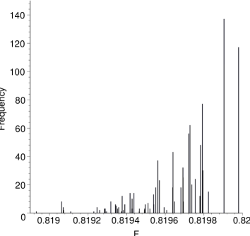
Figure 1: Local maxima of one of the $8^{4}$ SU(3), $\beta=5.7$, configurations after 1000 Steepest Descent starting from random points ($\theta\leq 10^{-10}$).

The combined evolutionary algorithm steepest descent method (CEASD) has a large number of parameters and to establish the algorithm we tried to cover, as much as possible, the space of parameters. Table 1 is a summary of the various runs. All results reported in this paper, for this smaller lattice, consider runs with 400 generations and use $N_{ipop}\leavevmode\nobreak\$= $2.5\leavevmode\nobreak\ \times\leavevmode\nobreak\$$N_{pop}\leavevmode\nobreak\$, $N_{good}\leavevmode\nobreak\$= $N_{pop}\leavevmode\nobreak\$/2 and $N_{elite}\leavevmode\nobreak\$= 1.

$N_{ipop}\leavevmode\nobreak\$	10	20	30	40	50
$N_{pop}\leavevmode\nobreak\$	4	8	12	16	20
$N_{good}\leavevmode\nobreak\$	2	4	6	8	10

Table 1: Evolutionary populations considered on the $8^{4}$ study. The number of generations used in each run was 400.

For the combined algorithm, we observed that by increasing $N$ in (23), the computed maximum, i.e. the maximum computed after applying a SD to the best member of population of the last generation, becomes closer to the absolute maximum. Moreover, there is a minimum number of $N$, $N_{steps}\leavevmode\nobreak\$, such that the computed maximum of CEASD is the absolute maximum of $F_{U}$. Figure 2 reports the number of successful runs of the combined method, for the three $8^{4}$ test configurations, as function of $N_{ipop}\leavevmode\nobreak\$and $N$.

Figure 2 shows that, for each population size, there is a minimum value of $N$, $N_{steps}\leavevmode\nobreak\$, such that the CEASD algorithm correctly computes the absolute maximum. Figure 3 shows $N_{steps}\leavevmode\nobreak\$as a function of the initial population. The solid line is $N_{steps}\leavevmode\nobreak\$for 400 generations and the dashed line is the value of $N$ required to identify the absolute maximum in 50 generations. Results seem to suggest that for larger populations, $N_{steps}\leavevmode\nobreak\$should become smaller.

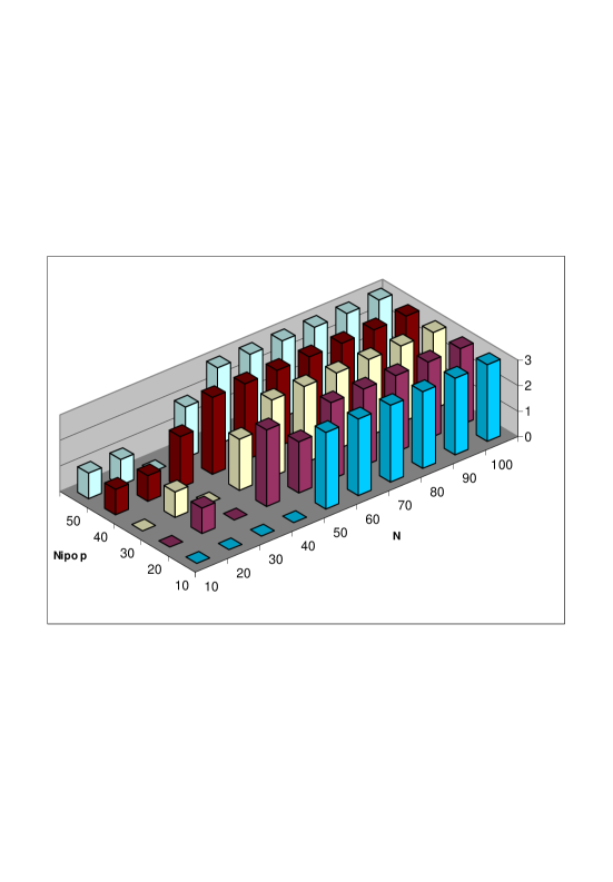
Figure 2: Number of successful runs for the combined method, for the three $8^{4}$ test configurations, as function of $N_{ipop}\leavevmode\nobreak\$and $N$.

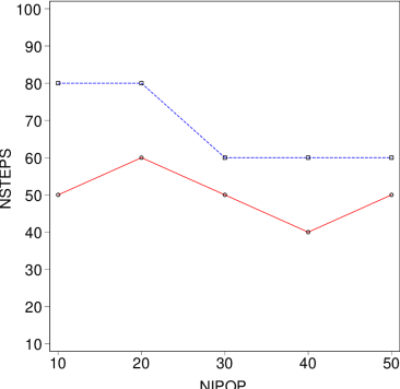
Figure 3: $N_{steps}\leavevmode\nobreak\$versus $N_{ipop}\leavevmode\nobreak\$for $8^{4}$ SU(3), $\beta=5.7$, configurations. The solid lines gives $N_{steps}\leavevmode\nobreak\$for 400 generations. The dashed line is $N_{steps}\leavevmode\nobreak\$for 50 generations.

Table 2 reports the first generation that includes the absolute maximum in the population. The results seems to suggest that, for an $8^{4}$ lattice, 50 generations may be a safe number of generations for the CEASD algorithm to compute the absolute maximum of $F_{U}$.

Figure 4 reports, for different population sizes, typical evolutions of $\theta$ for one of the tested configurations. They show that, in each run, $\theta$ decreases rapidly in the first generations, with its value decreasing by roughly 3 to 4 orders of magnitude in the first 50 generations, and then remaining approximately constant. Moreover, in order to properly identify the absolute maximum of $F_{U}$, the algorithm seems to require $\theta\leavevmode\nobreak\ \sim\leavevmode\nobreak\ 10^{-6}-10^{-7}$ after generation 50.

\psfrag{EIXOX}{Generation}\psfrag{EIXOY}{$\log(\theta)$}\includegraphics[angle={-90},origin=c,scale={0.6}]{evolution_th_p10_s1.ps}

(a) $N_{ipop}\leavevmode\nobreak\$=10

\psfrag{EIXOX}{Generation}\psfrag{EIXOY}{$\log(\theta)$}\includegraphics[angle={-90},origin=c,scale={0.6}]{evolution_th_p20_s1.ps}

(b) $N_{ipop}\leavevmode\nobreak\$=20

\psfrag{EIXOX}{Generation}\psfrag{EIXOY}{$\log(\theta)$}\includegraphics[angle={-90},origin=c,scale={0.6}]{evolution_th_p40_s1.ps}

(c) $N_{ipop}\leavevmode\nobreak\$=40

\psfrag{EIXOX}{Generation}\psfrag{EIXOY}{$\log(\theta)$}\includegraphics[angle={-90},origin=c,scale={0.6}]{evolution_th_p50_s1.ps}

(d) $N_{ipop}\leavevmode\nobreak\$=50

Figure 4: $\log(\theta)$ for one of the $8^{4}$ test configurations and different population sizes. The value of N is represented by the thickness of the line (larger thickness meaning larger $N$).

	$N_{ipop}\leavevmode\nobreak\$
$N_{steps}\leavevmode\nobreak\$	10	20	30	40	50
10	-	-	-	-	-
20	-	-	-	-	-
30	-	-	-	-	-
40	-	100	-	100	-
50	150	-	150	150	150
60	150	50	50	50	50
70	350	100	50	50	50
80	50	50	50	50	50
90	50	50	50	50	50
100	50	50	50	50	50

Table 2: Number of generations required by the CEASD algorithm to identify the absolute maximum for an $8^{4}$ lattice.

In conclusion, for an $8^{4}$ lattice it is possible to define a set of parameters such that the CEASD algorithm identifies the gauge transformation that maximizes $F_{U}$. For this smaller lattice, our choice being $N_{steps}\leavevmode\nobreak\$= 100, $N_{ipop}\leavevmode\nobreak\$= 10 for runs with 200 generations. Note that from figure 3 one reads $N_{steps}\leavevmode\nobreak\$= 50. However, since evolutionary algorithms are statistical algorithms and the combined algorithm requires a relatively low value for $\theta$ to access the absolute maximum of $F_{U}$, our choice for $N_{steps}\leavevmode\nobreak\$and the number of generations was conservative. Indeed, results show that similar results can be obtained for runs with only 50 generations. Decreasing the number of generations implies either increasing $N_{steps}\leavevmode\nobreak\$(increasing the computational cost of the cost function), increasing $N_{ipop}\leavevmode\nobreak\$(increasing the memory requirements) or relying on multiple runs of the algorithm. Of course, the user should choose between the different possible solutions depending on the computational power he has available.

In order to get an idea on the cpu time required by the CEASD, we benchmarked the code on a Pentium IV at 2.40 GHz. For the $8^{4}$ lattice, $N_{steps}\leavevmode\nobreak\$= 100, $N_{ipop}\leavevmode\nobreak\$= 10 and requiring $\theta\,<\,10^{-15}$ for the final steepest descent applied to the best member of the population of the last generation, we measured

number of generations		cpu time (s)
50		2633
200		10859

meaning that the CEASD algorithm requires about 54 seconds/generation. For the same gauge fixing precision, the steepest descent method requires 56 seconds. Therefore, the time required by a run with 200 generations is similar to the time required by 200 multiple steepest descent. At this point, a warning should be given to the reader. The CEASD code has space for optimization, therefore the cpu times reported above should be read as order of magnitudes. The CEASD memory requirements for the evolutive phase ($N_{pop}\leavevmode\nobreak\$= 4) are about 15MB.

In the next section we report on the CEASD algorithm for a larger lattice.

4.2 $16^{4}$ lattices

\psfrag{EIXOX}{Generation}\psfrag{EIXOY}{$\log(\theta)$}\includegraphics[angle={-90},scale={0.7}]{su3_fmax_16_9000.ps}

Figure 5: Local maxima of a $16^{4}$ SU(3), $\beta=6.0$ configuration achieved after 500 Steepest Descent starting from random starting points ($\theta\leq 10^{-15}$). For the three configurations used to set the algorithm, the number of different Gribov copies found after 500 SD was 177/500, 238/500, 326/500 for configurations number 66000, 72000 and 9000, respectively.

For the larger lattice considered in this work, seven $\beta\,=\,6.0$ gauge configurations were generated. Similarly to what was done for the $8^{4}$ lattice, the Gribov copies structure was studied applying 500 steepest descents started from different randomly chosen points. In order to test the algorithm we performed a detailed study for the three configurations with the largest number of Gribov copies.

The first observation being that the number of local maxima is now much larger than in the $8^{4}$ lattice. Figure 5 shows the Gribov copies found in 500 multiple SD of one of the configurations used in the detailed study of the CEASD algorithm. A similar figure for a $8^{4}$ configuration is figure 1. Not only, the number of local maxima increases but also the maxima become closer to each other when compared to the smaller lattice. To give an idea of the local maxima for the $16^{4}$ configurations, in table 3 we list the first five highest values of $F_{U}$ computed after the 500 SD method, the 10${}^{\mbox{th}}$ and the smaller $F_{U}$. From the numerical point of view, this difference makes the global optimization problem a much harder problem to solve. Concerning the frequency of the local maxima, the results for the $16^{4}$ and $8^{4}$ lattices are similar. The most probable maxima are associated with the largest values of $F_{U}$ but the copy with the largest frequency is not always the absolute maximum of $F_{U}$.

	Conf66000	Freq.	Conf72000	Freq.	Conf9000	Freq.
1	0.86013650	17	0.85964596	15	0.85962982	6
2	0.86013552	3	0.85963938	2	0.85962880	13
3	0.86013533	8	0.85963928	7	0.85961392	13
4	0.86013430	10	0.85963888	5	0.85961286	1
5	0.86013269	6	0.85963756	1	0.85961242	4
10	0.86012155	6	0.85963328	4	0.85960036	1
smaller	0.85907152	1	0.85866489	1	0.85885161	1

Table 3: $F_{U}$ values after 500 SD - $16^{4}$ lattice.

For the larger lattice, the investigation of the algorithm did not cover the same set of parameters as in the study of the smaller lattice. Indeed, due to the difference on the size of a gauge configuration, a factor of $2^{4}$, we only considered the smallest population sizes, namely $N_{ipop}\leavevmode\nobreak\$= 10, 20. The larger populations were avoided because of the large memory requirements. In what concerns the number of generations on each run, for the larger lattice we only considered runs up to 200 generations and checked for the presence of to the best maximum each 50 generations. As in the previous section, in all runs we used $N_{ipop}\leavevmode\nobreak\$= 2.5$N_{pop}\leavevmode\nobreak\$.

	$N_{ipop}\leavevmode\nobreak\$	10			20
$N$	Generation	66000	72000	9000	66000	72000	9000
120	50	1	4	2	1	4	1
	100	1	3	2	1	1	1
	150	1	3	2	1	1	1
	200	1	3	2	1	1	1
130	50	1	3	6	1	2	1
	100	1	1	2	1	2	1
	150	1	1	2	1	2	1
	200	1	1	2	1	1	1
140	50	3	9	2	1	1	2
	100	1	9	1	1	1	2
	150	1	6	1	1	1	2
	200	1	1	1	1	1	2
150	50	3	3	1	1	1	1
	100	1	3	1	1	1	1
	150	1	3	1	1	1	1
	200	1	3	1	1	1	1
160	50	1	1	2	2	1	1
	100	1	1	2	2	1	1
	150	1	1	2	2	1	2
	200	1	1	2	1	1	2
170	50	1	1	2	1	1	1
	100	1	1	2	1	1	1
	150	1	1	2	1	1	1
	200	1	1	2	1	1	1
180	50	1	1	1	2	1	2
	100	1	1	1	1	1	2
	150	1	1	1	1	1	1
	200	1	1	1	1	1	1
190	50	1	$>$ 9	3	1	1	1
	100	1	1	1	1	1	1
	150	1	1	1	1	1	1
	200	1	1	1	1	1	1
200	50	1	7	1	1	1	2
	100	1	2	1	1	1	2
	150	1	1	1	1	1	1
	200	1	1	1	1	1	1

Table 4: Maxima computed with the CEASD algorithm for three $16^{4}$, $\beta=6.0$ SU(3) configurations.

In table 4 we summarize the performance of the algorithm for the three gauge configurations considered. For the smallest population, the algorithm seems to identify the absolute maximum in 200 generations for $N\,\geq\,180$ ($N_{steps}\leavevmode\nobreak\$= 180). For runs up to 50 generations, when $N_{ipop}\leavevmode\nobreak\$= 10 the algorithm sometimes fails the computation of the absolute maximum. For runs up to 50 generations and $N\,\geq\,180$, the probability of getting the absolute maximum is $p_{max}\,=\,0.67$ for $N_{ipop}\leavevmode\nobreak\$= 10. The probability of getting a maximum which is not the absolute maximum in $K$ independent runs is then $p_{other}\,=\,0.33^{K}$, a number which goes rapidly to zero with $K$. Therefore, it seems reasonable to try the use of smaller number of generations, provided multiple independent runs of the algorithm are done. A possible improvement of the multiple run situation could be a parallel version of the CEASD algorithm, with the interchange of chromosomes between the essentially independent populations every now and then. For the largest population, $N_{ipop}\leavevmode\nobreak\$= 20, the algorithm identifies the absolute maximum when 200 generations are considered for $N\,\geq\,170$ ($N_{steps}\leavevmode\nobreak\$= 170). For runs up to 50 generations, again, the algorithm does not provide the right maximum. Now, $p_{max}\,=\,0.75$ for $N_{ipop}\leavevmode\nobreak\$= 20 and the situation becomes similar to case discussed previously. Once more, multiple runs of the CEASD algorithm should be able to identify the absolute maximum of $F_{U}$ when using 50 generations.

In conclusion, if for runs up 50 generations only a multiple independent run can provide the right answer, when the algorithm uses 200 generations, it is possible to define $N_{steps}\leavevmode\nobreak\$:

$N_{ipop}\leavevmode\nobreak\$		$N_{steps}\leavevmode\nobreak\$
10		180
20		170.

To close this section we report now on the cpu times. On a Pentium IV at 2.40 GHz, for a $16^{4}$ lattice, $N_{steps}\leavevmode\nobreak\$= 200, $N_{ipop}\leavevmode\nobreak\$= 10 and for $\theta\,<\,10^{-15}$ the cpu time measured required by the CEASD algorithm was

number of generations		cpu time (s)
50		112090
200		436071

meaning that the CEASD algorithm requires about 2211 seconds/generation. For the same gauge fixing precision, the steepest descent method requires 1826 seconds. Then, the time required by a run with 200 generations is similar to the time required by 240 multiple steepest descent. The CEASD memory requirements for the evolutive phase ($N_{pop}\leavevmode\nobreak\$= 4) are about 236MB.

5 Discussion and Conclusions

In this paper we describe a method for Landau gauge fixing that combines an evolutionary algorithm with a local optimization method. The “happy marriage” between the two algorithms is achieved by redefining the cost function of the EA, in such a way that it becomes an approximation for the local maximum in the neighborhood of the chromosome. In order to get the global maximum, the CEASD algorithm seems to require values for $\theta$ of the order of $10^{-7}$ for $8^{4}$ configurations and $10^{-8}$ for $16^{4}$ configurations. Note that the CEASD requires only a good approximation of $F_{U}$ in order to be able to compute the global optimum.

The combined algorithm was tested for three different configurations in two lattices: a smaller $8^{4}$ lattice and a larger $16^{4}$ lattice. For both lattices it was possible to identify a set of parameters for the CEASD method such that, in a single run, the computed maximum, i.e. the maximum obtained after applying the steepest descent method to best member of the population of the last generation, was always the global maximum defined from multiple steepest descent runs.

For the smaller lattice the CEASD performed extremely well. Indeed, despite the relative large number of local maxima, the algorithm seems to be quite stable in identifying the global maximum of $F_{U}$ - see table 2. For the larger lattice, the number of local maxima is much larger when compared to the $8^{4}$ lattice. Not only the number of maxima is larger but they are closer to each other. From the point of view of the global optimization, this means that the numerical problem in hands is much harder to solve. Nevertheless, again it was possible to define a set of parameters such that the algorithm identified the global maximum in all tested configurations - see table 4. Our choice of parameters for the CEASD algorithm (200 generations, $N_{steps}\leavevmode\nobreak\$= 100 for $8^{4}$ lattice and $N_{steps}\leavevmode\nobreak\$= 200 for the larger lattice and for $N_{ipop}\leavevmode\nobreak\$= 10) is a conservative choice. As explained before, it is possible to use smaller values of $N$ or smaller number of generations. Decreasing $N$ and/or the number of generations implies decreasing the run time of the CEASD algorithm. However, reducing $N$ and/or the number of generations should be done with care. Indeed, the comparative study of the two lattices shows that the complexity of the maximisation problem increases with the lattice size, that the method works better for larger populations, larger values of $N$ and for sufficiently large number of generations. Nevertheless, the results of the previous section also show that, for relatively large values of $N$, the probability of computing the absolute maximum of $F_{U}$ is large. This suggests that a possible solution to the global optimization problem is to perform multiple independent CEASD runs using lower values of $N$ and/or smaller number of generations. For sufficient number of independent runs, in principle, the method should be able to get the global maximum. A similar situation is found when one relies on simulated annealing for global optimization problems.

The cpu times required by CEASD algorithm for the two lattice sizes seems to suggest that the scaling law of the combined method is close to the Fourier accelerated SD method, i.e. $V^{\delta}\,\ln V$ with $\delta$ taking values close to 1. A measure of $\delta$ requires necessarily an analysis with more lattice sizes. This is a numerical intensive problem. We are currently engaged in measuring $\delta$ and will report the result elsewhere. Naïvely, one expects that gauge fixing to the minimal Landau gauge with CEASD is as demanding as performing a gauge fixing with the SD method.

In principle, it is possible to combine the EA with any local optimisation method. Faster local methods will produce faster combined algorithms. The time required by a combined algorithm is strongly dependent on the performance of the local method. The gauge fixing is a computational intense problem. Therefore, it is important to investigate new and more performant local methods.

The CEASD algorithm described here for Landau gauge fixing seems to solve the problem of the minimal Landau gauge fixing. Moreover, the method is suitable to be used with other gauge conditions that also suffer from the Gribov ambiguity and are currently used in lattice gauge theory. The effects of Gribov copies in QCD correlation functions remains to be investigated nosso .

P. J. S. acknowledges financial support from the portuguese FCT. This work was in part supported by fellowship Praxis/P/FIS/14195/98 under project Optimization in Physics and in part from grant SFRH/BD/10740/2002.

References

- (1) see for example, I. Montvay, G. Münster, Quantum Fields on a Lattice, CUP 1994.
- (2) R. P. Feynman Acta Phys. Pol. 24 (1963) 262.
- (3) B. DeWitt, Phys. Rev. 160 (1967) 113; Phys. Rev. 162 (1967) 1195; Phys. Rev. 162 (1967) 1293.
- (4) L. P. Faddeev, V. N. Popov, Phys. Lett. B25 (1967) 29.
- (5) V. N. Gribov, Nucl. Phys. B139 (1978) 1.
- (6) S. Sciuto, Phys. Rep. 49 (1979) 181.
- (7) I. M. Singer, Comm. Nucl. Phys. 60 (1978) 7.
- (8) T. P. Killingback, Phys. Lett. B138 (1983) 87.
- (9) D. Zwanziger, hep-ph/0303028.
- (10) D. Zwanziger, Nucl. Phys. B364 (1991) 127.
- (11) R. Alkofer, W. Detmold, C. S. Fischer, P. Maris, hep-ph/0309077; hep-ph/0309078.
- (12) R. Alkofer, C. S. Fischer, hep-ph/0309089.
- (13) C. T. H. Davies et al, hep-lat/0304004.
- (14) G. Martinelli, C. Pittori, C. T. Schrajda, M. Testa, A. Vladikas Nucl. Phys. B445 (1995) 81.
- (15) For a general overview of gauge fixing in lattice gauge theories and related issues see L. Giusti, M. C. Paciello, C. Parrinello, S. Petrarca, B. Taglienti, Int. J. Mod. Phys. A16 (2001) 3487 [hep-lat/0104012].
- (16) C. H. T. Davies, G. G. Batrouni, G. P. Katz, A. S. Kronfeld, G. P. Lepage, P. Rossi, B. Svetitsky and K. G. Wilson, Phys. Rev. D37 (1988) 1581.
- (17) For evolutionary algorithms see, for example, the following books GA_Mich GA_Coley GA_Raupt .
- (18) Zbigniew Michalewicz, Genetic Algorithms + Data Structures = Evolution Programs, Springer, 1996.
- (19) D. A. Coley, An Introduction to Genetic Algorithms for Scientists and Engineers, World Scientific Publishing, 1999.
- (20) R. L. Raupt, S. E. Raupt, Practical Genetic Algorithms, J. Wiley & Sons, 1998.
- (21) O. Oliveira, P. J. Silva, Nucl. Phys. B(Proc. Suppl.)106 (2002) 1088 [hep-lat/0110035].
- (22) Semyonov-Tian-Shansky, Franke, Proc. Seminars of the Leningrad Math. Inst., 1982 (Plenum, New York, 1986) [English translation].
- (23) G. Dell’Antonio, D. Zwanziger, Comm. Math. Phys. 138 (1991) 291.
- (24) P. van Baal, Nucl. Phys. B369 (1992) 259.
- (25) P. van Baal, Nucl. Phys. B417 (1994) 215.
- (26) P. van Baal, hep-th/9511119.
- (27) D. Zwanziger, Nucl. Phys. B378 (1992) 525.
- (28) D. Zwanziger, Nucl. Phys. B412 (1994) 657.
- (29) A. Cucchieri,Nucl. Phys. B521 (1998) 365 [hep-lat/9711024].
- (30) A. Nakamura, R. Sinclair, Phys. Lett. BB243 (1990) 396.
- (31) P. de Forcrand, Nucl. Phys. B(Proc. Suppl.)20 (1991) 194.
- (32) E. Marinari, C. Parrinello, R. Ricci, Nucl. Phys. B362 (1991) 487.
- (33) A. Cucchieri, Nucl. Phys. B508 (1997) 353 [hep-lat/9705005].
- (34) S. Furui, H. Nakajima, hep-lat/0309166.
- (35) O. Oliveira, P. J. Silva, Gribov copies and the gluon propagator, communication at I Portuguese Hadronic Physics National Meeting, Lisbon 2003.
- (36) O. Oliveira, P. J. Silva, in preparation.
- (37) J.E.Mandula, M.Ogilvie Phys. Lett. B248 (1990) 156.
- (38) A. Cucchieri, T. Mendes, Phys. Rev. D57 (1998) 3822 [hep-lat/9711047].
- (39) A. Cucchieri, T. Mendes, Nucl. Phys. Proc. Suppl. 63 (1998) 841 [hep-lat/9710040].
- (40) A. Yamaguchi, H. Nakajima, hep-lat/9909064.
- (41) J. F. Markham, T. D. Dieu, hep-lat/9809143.
- (42) This work was in part based on the MILC collaboration’s public lattice gauge theory code. See http://physics.indiana.edu/~sg/milc.html.