Large Mass and Chemical Potential Model: A Laboratory for QCD?

Abstract

We use a model based on the hopping parameter expansion to study QCD at large $\mu$. We find interesting behavior in the region expected to show flavor-color locking.

Motivation and problem setting While the analysis for QCD at small $\mu$ and large $T$ gradually improves, there are no studies yet at large $\mu$ and small $T$. Results hereto have only been obtained in models which are not directly derivable from QCD, such as SU(2) and isovector chemical potential, or NJL. Here we want to approach this very interesting region [1] in a model which can be obtained as large mass, large chemical potential approximation of full QCD [2] and which in the static, dense quark limit [3] has been proposed as quenched formulation of QCD at finite baryon density [4]. See Fig. 1. For this we expand the fermion determinant in the inverse mass to second order, which ensures a limited mobility of the quarks. We use Wilson fermionic action and have for the hopping parameter:

$$\kappa=[2(M+3+\cosh\mu)]^{-1}=[2(M_{0}+4)]^{-1}$$

($M:$ bare mass, $M_{0}:$ bare mass at $\mu=0$). Then:

$${\cal Z}_{F}^{[2]}({{\kappa}},\mu,\left\{U\right\})={\rm exp}\left\{-2\,\sum_{\left\{{\vec{x}}\right\}}\,\sum_{s=1}^{\infty}\,{{{(\epsilon\,C)}^{s}}\over s}\right.{\times}$$

$$\left.{\rm Tr\,}\!\!\left[({\cal P}_{\vec{x}})^{s}+\kappa^{2}\sum_{r,q,i,t,t^{\prime}}(\epsilon\,C)^{s(r-1)}({\cal P}_{{\vec{x}},i,t,t^{\prime}}^{r,q})^{s}\right]\right\}\!\!$$ (1)

$$={\cal Z}_{F}^{[0]}(C,\left\{U\right\})\!\!\!\!\!\!\prod_{{\vec{x}},r,q,i,t,t^{\prime}}\!\!\!\!{\rm Det\,}\left(1-(\epsilon\,C)^{r}\,\kappa^{2}\,{\cal P}_{{\vec{x}},{i},t,t^{\prime}}^{r,q}\right)^{2},$$

$$C=(2\zeta)^{N_{\tau}},\ \ \zeta=\kappa\,e^{\mu}$$ (2)

In the temporal gauge ($U_{n,4}=1$, except for $U_{({\vec{x}},n_{4}=N_{\tau}),4}\equiv V_{\vec{x}}$: free) we have ${\cal P}_{\vec{x}}=V_{\vec{x}}$ and

$${\cal P}_{{\vec{x}},i,t,t^{\prime}}^{r,q}=(V_{\vec{x}})^{r-q}U_{({\vec{x}},t),i}(V_{{\vec{x}}+{\hat{\i}}})^{q}U_{({\vec{x}},t^{\prime}),i}^{*}$$ (3)

with $r>q\geq 0$, $i=\pm 1,\pm 2,\pm 3$, $1\leq t\leq t^{\prime}\leq N_{\tau}$ ($t<t^{\prime}$ for $q=0$). Here $\epsilon=1\,(-1)$ for p.b.c. (a.p.b.c). For detail see [2].

The hope is that the model retains some features of QCD in the large $\mu$ region, and that due to the simplicity of the determinant large statistics reweighting methods could converge, giving insight in the phase structure of QCD.

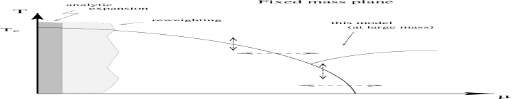
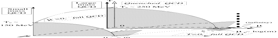
Figure 1: Tentative phase diagram of QCD.

One flavor QCD The simulations used here and below are done on a $6^{4}$ periodic lattice (a.p.b.c. for fermions in $\tau$-direction, Wilson plaquette action for the gauge field). The algorithm uses a local Boltzmann factor obtained by taking out from ${\cal Z}_{F}^{[2]}$ the factor

$$\prod_{\vec{x}}{\rm exp}\left\{2C{\cal R}e{\rm Tr\,}\left[{\cal P}_{\vec{x}}+\kappa^{2}\sum_{r,q,i,t,t^{\prime}}{\cal P}_{{\vec{x}},i,t,t^{\prime}}^{r,q}\right]\right\}$$

compensating for this in the global reweighting (both procedures are vectorized). We use temporal gauge fixing for easy book-keeping of the contributions to ${\cal Z}_{F}^{[2]}$. We first analyze one flavor QCD, some results are shown in Fig. 2. The convergence appears rather good, up to very large $n_{B}$ (baryon density over $T^{3}$; $n_{B}(sat)=216$). Both $n_{B}$ and Polyakov loop increase above $\mu\sim 1$.

Figure 2: One flavor QCD. Upper plot: iteration history for $n_{B}$. Lower plot: $n_{B}/n_{B}(sat)$ and Polyakov loop vs $\mu$.

Application to QCD with three degenerate flavors: Color-flavor locking We now investigate whether a transition to a phase, where the ground state is characterized by a color-flavor locking condensate of quark bilinears [1], takes place. Disregarding the possibility of parity violation in the ground state, such a condensate most generally is parameterized as

$$\left\langle\psi^{a}_{i}C\gamma^{5}\psi^{b}_{j}\right\rangle=K_{1}\,\delta^{a}_{i}\delta^{b}_{j}+K_{2}\,\delta^{a}_{j}\delta^{b}_{i}\,$$ (4)

where $C=i\gamma_{2}\gamma_{0}$ is the charge conjugation matrix. The contraction of Dirac indices is implicit while $a\cdots h$ and $i\cdots z$ denote color and flavor indices, respectively. The condensate is invariant under locked global color and vectorial flavor rotations. To project out the invariants $K_{1}$ and $K_{2}$ we apply $\lambda\left(\delta_{i}^{a}\delta^{b}_{j}+\rho\,\delta^{a}_{j}\delta^{b}_{i}\right)$ to the condensate (4) with $(\lambda,\rho)=(-\frac{1}{36},-3)$ and $(\lambda,\rho)=(\frac{1}{8},-\frac{1}{3})$, respectively. We define the two-point correlator of color-flavor locking quark bilinears as $\left\langle\psi^{a}_{i}(x)C\gamma^{5}\psi^{b}_{j}(x)\left[\psi^{c}_{k}(0)C\gamma^{5}\psi^{d}_{l}(0)\right]^{\dagger}\right\rangle$. Two-point correlations of a certain combination of the invariants $K_{1,2}$ are obtained by applying

$$\lambda(x)\lambda(0)\left(\delta_{i}^{a}\delta^{b}_{j}+\rho(x)\,\delta^{a}_{j}\delta^{b}_{i}\right)\left(\delta_{k}^{c}\delta^{d}_{l}+\rho(0)\,\delta^{c}_{l}\delta^{d}_{k}\right)$$ (5)

to the above correlator after accordingly adjusting $(\lambda(x),\rho(x))$ and $(\lambda(0),\rho(0))$. In the Euclidean formulation the result can be decomposed as

$$\lambda(x)\lambda(0)\!\!\sum_{I,J=1,2}\!\!\left\langle\psi^{a}_{i}(x)O^{I,ab}_{ij}\psi^{b}_{j}(x)\bar{\psi}^{d}_{l}(0)\bar{O}^{J,cd}_{kl}\bar{\psi}^{c}_{k}(0)\right\rangle\$$

$$= O^{I}_{AB}\bar{O}^{J}_{CD}\,\left(W^{-1}_{A,C}(x,0)W^{-1}_{B,D}(x,0)\right.$$ (6)

$$- \left.W^{-1}_{A,D}(x,0)W^{-1}_{B,C}(x,0)\right)\,\det W$$

(see, e.g., see for example [5]), where

$$O^{1,ab}_{ij} = \delta_{i}^{a}\delta^{b}_{j}\gamma_{2}\gamma_{4}\gamma_{5},\ O^{2,ab}_{ij}=\rho(x)\delta_{j}^{a}\delta^{b}_{i}\gamma_{2}\gamma_{4}\gamma_{5}\,,$$

$$\bar{O}^{1,cd}_{kl} = \delta_{k}^{c}\delta_{l}^{d}\gamma_{5}\gamma_{4}\gamma_{2},\ \bar{O}^{2,cd}_{kl}=\rho(0)\delta_{l}^{c}\delta_{k}^{d}\gamma_{5}\gamma_{4}\gamma_{2}$$

Here a ’super’ index $A=(\alpha,a,i)$ was introduced with $\alpha$ a Dirac index. Like $\det W$ $W^{-1}$ can also be expanded in powers of $\kappa$ [2], the paths contributing to ${\cal O}(\kappa^{2})$ are shown in Fig. 3.

Figure 3: Paths contributing to ${\cal O}(\kappa^{2})$.

We have performed simulations for QCD with 3 degenerate flavors at $\beta=5.6$ on a $6^{4}$ lattice at $\kappa=0.12$ and various $\mu$ (same for all flavors). Results are shown in Fig. 4. The general convergence is poorer than for the 1-flavor case at same $\mu$. In particular, the region around $\mu=1$ acknowledges strong fluctuations, while at larger $\mu$ the situation improves again. Here we also measure the “QQ”-susceptibility obtained by integrating the correlator of $K_{1}+\xi\,K_{2}$ (6), where for definiteness we chose $\xi=0.5$. For this quantity we use maximal gauge fixing. The $\kappa^{2}$ contribution appears essential for the non-trivial large $\mu$ behavior (the ”mobility” defined as the ${\cal O}(\kappa^{2})$ fraction of $n_{B}$ over total $n_{B}$ is typically $\sim 0.3$).

Figure 4: 3-flavor QCD. Upper plot: Iteration history for $n_{B}$ at $\mu=0.85$ (multiplied by 10) and $1.08$. Lower plot: “QQ”-susceptibility to ${\cal O}(\kappa^{0})$ (multiplied by 5) and to ${\cal O}(\kappa^{2})$, vs $\mu$.

Conclusions and outlook We have performed simulations at small $T$, large $\mu$ for a model which can be obtained from QCD by small order hopping parameter expansion at large $\mu$. The quarks, although very heavy, have some limited amount of mobility. The results show strong increase of the baryon density and other observables above $\mu\sim 1$ which may be a signal for entering a new, high density phase at small temperature. Particularly interesting is the behavior of the di-quark correlator in 3-flavor QCD which becomes increasingly flat at large $\mu$, leading to a strongly increasing susceptibility. This may be a signal for the development of a condensate with color-flavor locking. Simulations on larger lattices would be essential to check this conjecture, it remains to be seen whether good convergence can be achieved in that case.

Acknowledgments The calculations have been performed on the VPP5000 of the Forschungszentrum Karlsruhe and the University Karlsruhe.

References

• [1] M. G. Alford, K. Rajagopal, and F. Wilczek, Nucl. Phys. B537, 443 (1999).
• [2] G.Β Aarts, O.Β Kaczmarek, F.Β Karsch and I.-O.Β Stamatescu, Nucl. Phys. B (Proc.Suppl.) 106 (2002) 456.
• [3] I.Β Bender et al., Nucl.Β Phys.Β Proc.Β Suppl.Β  26 (1992) 323.
• [4] Engels et al, Nucl. Phys. B 558 (1999) 307.
• [5] C. B. Lang and H. Nicolai, Nucl. Phys. B200[FS4], 135 (1982).