A Perturbative Determination of
Mass Dependent $O(a)$ Improvement Coefficients
in a Relativistic Heavy Quark Action

Abstract

We present the results for a perturbative determination of mass dependent improvement coefficients $\nu$, $r_{s}$, $c_{E}$ and $c_{B}$ in a relativistic heavy quark action, which we have designed to control $m_{Q}a$ errors by extending the on-shell $O(a)$ improvement program to the case of $m_{Q}\gg\Lambda_{\rm QCD}$, where $m_{Q}$ is the heavy quark mass. The parameters $\nu$ and $r_{s}$ are determined from the quark propagator and $c_{E}$ and $c_{B}$ are from the on-shell quark-quark scattering amplitude. We show that all the parameters, together with the quark wave function and the mass renormalization factors, are determined free from infrared divergences once their tree level values are properly tuned. Results of these parameters are shown as a function of $m_{Q}a$ for various improved gauge actions.

I Introduction

A calculation of weak matrix elements for the $B$ and $D$ mesons is a subject of great interest in lattice QCD: their precise determination is an essential ingredient to extract the Cabibbo-Kobayashi-Maskawa matrix. Although in principle we can extract these weak matrix elements precisely from lattice QCD simulations, it is still difficult to achieve this goal. A main obstacle is the systematic error originating from large $m_{Q}a$ corrections with current accessible computational resources: $m_{b}a\sim 1-2$ and $m_{c}a\sim 0.3-0.6$ in the quenched approximation and $m_{b}a\sim 2-3$ and $m_{c}a\sim 0.6-0.9$ in unquenched QCD.

To control this large $m_{Q}a$ corrections a new relativistic approach is proposed from the view point of the on-shell $O(a)$ improvement programakt . The generic quark action is given by

$$S_{q} = \sum_{x}\left[m_{0}{\bar{q}}(x)q(x)+{\bar{q}}(x)\gamma_{0}D_{0}q(x)+\nu\sum_{i}{\bar{q}}(x)\gamma_{i}D_{i}q(x)\right.$$ (1)

$$\left.-\frac{r_{t}a}{2}{\bar{q}}(x)D_{0}^{2}q(x)-\frac{r_{s}a}{2}\sum_{i}{\bar{q}}(x)D_{i}^{2}q(x)\right.$$

$$\left.-\frac{iga}{2}c_{E}\sum_{i}{\bar{q}}(x)\sigma_{0i}F_{0i}q(x)-\frac{iga}{4}c_{B}\sum_{i,j}{\bar{q}}(x)\sigma_{ij}F_{ij}q(x)\right],$$

where we are allowed to choose $r_{t}=1$ and other four parameters $\nu$, $r_{s}$, $c_{E}$ and $c_{B}$ are analytic functions of $m_{Q}a$ and the gauge coupling constant $g$.

In this formulation the leading cutoff effects of order $(m_{Q}a)^{n}$ are absorbed in the definition of renormalization factors for the quark mass and the wave function. After removing the next-leading cutoff effects of $O((m_{Q}a)^{n}a{\Lambda}_{\rm QCD})$ with $\nu$, $r_{s}$, $c_{E}$ and $c_{B}$ in the quark action properly adjusted in the $m_{Q}a$ dependent way, we are left with at most $O((a{\Lambda}_{\rm QCD})^{2})$ errors.

In this paper we calculate $\nu$, $r_{s}$, $c_{E}$ and $c_{B}$ up to the one-loop level for various improved gauge actions. While $\nu$ and $r_{s}$, together with the quark wave function renormalization factor $Z_{q}$ and the pole mass $m_{p}$ as byproducts, are obtained from the quark propagator, $c_{E}$ and $c_{B}$ are determined from the on-shell quark-quark scattering amplitude. One-loop diagrams are evaluated by employing the conventional perturbative method with the use of the fictitious gluon mass to regularize the infrared divergence, which was successfully applied in the massless case to the calculation of the renormalization constants and the improvement coefficients for the quark bilinear operatorsgmass and the improvement coefficient ${c_{\rm SW}}$csw_m0 . We show that the improvement parameters $\nu$, $r_{s}$, $c_{E}$ and $c_{B}$ are determined free from the infrared divergences, once their tree level values are correctly tuned in the $m_{Q}a$ dependent way. Some preliminary results are presented in Ref. latt02 .

This paper is organized as follows. In Sec. II we introduce the relativistic heavy quark action and the improved gauge actions. We also give their Feynman rules relevant for the present calculation. We describe the method for the calculation of the one-loop diagrams in Sec. III. In Sec. IV we determine $\nu$ and $r_{s}$ from the quark propagator. The results for $Z_{q}$ and $m_{p}$ are also presented. In Sec. V ${\it c}_{\it B}$ and ${\it c}_{\it E}$ are determined from the on-shell quark-quark scattering amplitude. We give a rather detailed description on the cancellation of the infrared divergences in one-loop diagrams. In Sec. VI we explain how to implement the mean field improvement of the parameters. Our conclusions are summarized in Sec. VII.

The physical quantities are expressed in lattice units and the lattice spacing $a$ is suppressed unless necessary. We take SU($N_{c}$) gauge group with the gauge coupling constant $g$.

II Action and Feynman Rules

The relativistic heavy quark action proposed in Ref. akt is given by

$$S_{\rm quark} = \sum_{n}\frac{1}{2}\left\{{\bar{\psi}}_{n}(-r_{t}+\gamma_{0})U_{n,0}\psi_{n+{\hat{0}}}+{\bar{\psi}}_{n}(-r_{t}-\gamma_{0})U^{\dagger}_{n-{\hat{0}},0}\psi_{n-{\hat{0}}}\right\}$$ (2)

$$+\sum_{n}\frac{1}{2}\sum_{i}\left\{{\bar{\psi}}_{n}(-r_{s}+\nu\gamma_{i})U_{n,i}\psi_{n+{\hat{i}}}+{\bar{\psi}}_{n}(-r_{s}-\nu\gamma_{i})U^{\dagger}_{n-{\hat{i}},i}\psi_{n-{\hat{i}}}\right\}$$

$$+(m_{0}+r_{t}+3r_{s})\sum_{n}{\bar{\psi}}_{n}\psi_{n}$$

$$-{\it c}_{\it E}\sum_{n}\sum_{i}ig\frac{1}{2}{\bar{\psi}}_{n}\sigma_{0i}F_{0i}(n)\psi_{n}-{\it c}_{\it B}\sum_{n}\sum_{i,j}ig\frac{1}{4}{\bar{\psi}}_{n}\sigma_{ij}F_{ij}(n)\psi_{n},$$

where we define the Euclidean gamma matrices in terms of the Minkowski ones in the Bjorken-Drell convention: $\gamma_{0}=\gamma_{BD}^{0}$, $\gamma_{j}=-i\gamma_{BD}^{j}$ $(j=1,2,3)$, $\gamma_{5}=\gamma_{BD}^{5}$ and $\sigma_{\mu\nu}=\frac{1}{2}[\gamma_{\mu},\gamma_{\nu}]$. Whereas the value of $r_{t}$ can be chosen arbitrarily, $\nu$, $r_{s}$, ${\it c}_{\it E}$ and ${\it c}_{\it B}$ have to be adjusted to remove the cutoff effects of $O((m_{Q}a)^{n}a{\Lambda}_{\rm QCD})$. As explained in Ref. akt the $(m_{Q}a)^{n}$ corrections can be avoided by the redefinition of the quark field and mass. The field strength $F_{\mu\nu}$ in the clover term is expressed as

$$F_{\mu\nu}(n) = \frac{1}{4}\sum_{i=1}^{4}\frac{1}{2ig}\left(U_{i}(n)-U_{i}^{\dagger}(n)\right),$$ (3)

$$U_{1}(n) = U_{n,\mu}U_{n+{\hat{\mu}},\nu}U^{\dagger}_{n+{\hat{\nu}},\mu}U^{\dagger}_{n,\nu},$$ (4)

$$U_{2}(n) = U_{n,\nu}U^{\dagger}_{n-{\hat{\mu}}+{\hat{\nu}},\mu}U^{\dagger}_{n-{\hat{\mu}},\nu}U_{n-{\hat{\mu}},\mu},$$ (5)

$$U_{3}(n) = U^{\dagger}_{n-{\hat{\mu}},\mu}U^{\dagger}_{n-{\hat{\mu}}-{\hat{\nu}},\nu}U_{n-{\hat{\mu}}-{\hat{\nu}},\mu}U_{n-{\hat{\nu}},\nu},$$ (6)

$$U_{4}(n) = U^{\dagger}_{n-{\hat{\nu}},\nu}U_{n-{\hat{\nu}},\mu}U_{n+{\hat{\mu}}-{\hat{\nu}},\nu}U^{\dagger}_{n,\mu}.$$ (7)

The weak coupling perturbation theory is developed by writing the link variable in terms of the gauge potential

$$U_{n,\mu}=\exp\left(igaT^{A}A_{\mu}^{A}\left(n+\frac{1}{2}\hat{\mu}\right)\right),$$ (8)

where $T^{A}$ ($A=1,\dots,N^{2}_{c}-1$) is a generator of color SU($N_{c}$).

The quark propagator is obtained by inverting the Wilson-Dirac operator in eq.(2),

$$S_{q}^{-1}(p) = i\gamma_{0}{\rm sin}(p_{0})+\nu i\sum_{i}\gamma_{i}{\rm sin}(p_{i})+m_{0}$$ (9)

$$+r_{t}(1-{\rm cos}(p_{0}))+r_{s}\sum_{i}(1-{\rm cos}(p_{i})),$$

For the present calculation, we need one-, two- and three-gluon vertices with quarks:

$$V^{A}_{10}(p,q) = -gT^{A}\left\{i\gamma_{0}{\rm cos}\left(\frac{p_{0}+q_{0}}{2}\right)+r_{t}{\rm sin}\left(\frac{p_{0}+q_{0}}{2}\right)\right\},$$ (10)

$$V^{A}_{1i}(p,q) = -gT^{A}\left\{\nu i\gamma_{i}{\rm cos}\left(\frac{p_{i}+q_{i}}{2}\right)+r_{s}{\rm sin}\left(\frac{p_{i}+q_{i}}{2}\right)\right\},$$ (11)

$$V_{200}^{AB}(p,q) = \frac{a}{2}g^{2}\frac{1}{2}\{T^{A},T^{B}\}\left\{i\gamma_{0}\sin\left(\frac{p_{0}+q_{0}}{2}\right)-r_{t}\cos\left(\frac{p_{0}+q_{0}}{2}\right)\right\},$$ (12)

$$V_{2ii}^{AB}(p,q) = \frac{a}{2}g^{2}\frac{1}{2}\{T^{A},T^{B}\}\left\{\nu i\gamma_{i}\sin\left(\frac{p_{i}+q_{i}}{2}\right)-r_{s}\cos\left(\frac{p_{i}+q_{i}}{2}\right)\right\},$$ (13)

$$V_{300}^{ABC}(p,q) = \frac{a^{2}}{6}g^{3}\frac{1}{6}\left[T^{A}\{T^{B},T^{C}\}+T^{B}\{T^{C},T^{A}\}+T^{C}\{T^{A},T^{B}\}\right]$$ (14)

$$\times\left\{i\gamma_{0}\cos\left(\frac{p_{0}+q_{0}}{2}\right)+r_{t}\sin\left(\frac{p_{0}+q_{0}}{2}\right)\right\},$$

$$V_{3iii}^{ABC}(p,q) = \frac{a^{2}}{6}g^{3}\frac{1}{6}\left[T^{A}\{T^{B},T^{C}\}+T^{B}\{T^{C},T^{A}\}+T^{C}\{T^{A},T^{B}\}\right]$$ (15)

$$\times\left\{\nu i\gamma_{i}\cos\left(\frac{p_{i}+q_{i}}{2}\right)+r_{s}\sin\left(\frac{p_{i}+q_{i}}{2}\right)\right\},$$

$$V^{A}_{c1\mu}(p,q) = -gT^{A}\frac{1}{2}\sum_{\nu}{c_{\rm SW}}^{\mu\nu}\sigma_{\mu\nu}\cos\left(\frac{p_{\mu}-q_{\mu}}{2}\right)\sin(p_{\nu}-q_{\nu}),$$ (16)

$$V^{AB}_{c2\mu\nu}(p,q,k_{1},k_{2}) = -\frac{a}{2}g^{2}if_{ABC}T^{C}\frac{1}{4}$$

$$\times\left\{{c_{\rm SW}}^{\mu\nu}\sigma_{\mu\nu}\left[4\cos\left(\frac{k_{1\nu}}{2}\right)\cos\left(\frac{k_{2\mu}}{2}\right)\cos\left(\frac{q_{\mu}-p_{\mu}}{2}\right)\cos\left(\frac{q_{\nu}-p_{\nu}}{2}\right)\right.\right.$$

$$\left.\left.-2\cos\left(\frac{k_{1\mu}}{2}\right)\cos\left(\frac{k_{2\nu}}{2}\right)\right]\right.$$

$$\left.+\delta_{\mu\nu}\sum_{\rho}{c_{\rm SW}}^{\mu\rho}\sigma_{\mu\rho}\sin\left(\frac{q_{\mu}-p_{\mu}}{2}\right)\left[\sin(k_{2\rho})-\sin(k_{1\rho})\right]\right\},$$

$$V^{ABC}_{c3\mu\nu\tau}(p,q,k_{1},k_{2},k_{3}) = -3ig^{3}\frac{a^{2}}{6}$$

$$\times\left[T^{A}T^{B}T^{C}\delta_{\mu\nu}\delta_{\mu\tau}\sum_{\rho}i{c_{\rm SW}}^{\mu\rho}\sigma_{\mu\rho}\left\{-\frac{1}{6}\cos\left(\frac{q_{\mu}-p_{\mu}}{2}\right)\sin(q_{\rho}-p_{\rho})\right.\right.$$

$$\left.\left.+\cos\left(\frac{q_{\mu}-p_{\mu}}{2}\right)\cos\left(\frac{q_{\rho}-p_{\rho}}{2}\right)\cos\left(\frac{k_{3\rho}-k_{1\rho}}{2}\right)\sin\left(\frac{k_{2\rho}}{2}\right)\right\}\right.$$

$$\left.-\frac{1}{2}\left[T^{A}T^{B}T^{C}+T^{C}T^{B}T^{A}\right]i{c_{\rm SW}}^{\mu\nu}\sigma_{\mu\nu}\right.$$

$$\left.\times\left\{\delta_{\nu\tau}2\cos\left(\frac{q_{\mu}-p_{\mu}}{2}\right)\cos\left(\frac{q_{\nu}-p_{\nu}}{2}\right)\cos\left(\frac{k_{3\mu}+k_{2\mu}}{2}\right)\sin\left(\frac{k_{1\nu}}{2}\right)\right.\right.$$

$$\left.\left.+\delta_{\nu\tau}\sin\left(\frac{k_{3\nu}+k_{2\nu}}{2}\right)\cos\left(\frac{k_{1\mu}}{2}+k_{2\mu}\right)\right.\right.$$

$$\left.\left.+\delta_{\mu\tau}\sin\left(\frac{k_{1\mu}+2k_{2\mu}+k_{3\mu}}{2}\right)\cos\left(\frac{q_{\nu}-p_{\nu}}{2}\right)\cos\left(\frac{k_{3\nu}-k_{1\nu}}{2}\right)\right\}\right],$$

where ${c_{\rm SW}}^{0i}={c_{\rm SW}}^{i0}={\it c}_{\it E}$, ${c_{\rm SW}}^{ij}={\it c}_{\it B}$ $(i,j=1,2,3)$ and $f_{ABC}$ is the structure constant of SU($N_{c}$) gauge group. The first six vertices originate from the Wilson quark action and the last three from the clover term. The momentum assignments for the vertices are depicted in Fig. 1.

For the gauge action we consider the following general form including the standard plaquette term and six-link loop terms:

$$S_{\rm g}=\frac{1}{g^{2}}\left\{c_{0}\sum_{\rm plaquette}{\rm tr}U_{pl}+c_{1}\sum_{\rm rectangle}{\rm tr}U_{rtg}+c_{2}\sum_{\rm chair}{\rm tr}U_{chr}+c_{3}\sum_{\rm parallelogram}{\rm tr}U_{plg}\right\}$$ (19)

with the normalization condition

$$c_{0}+8c_{1}+16c_{2}+8c_{3}=1,$$ (20)

where six-link loops are composed of a $1\times 2$ rectangle, a bent $1\times 2$ rectangle (chair) and a three-dimensional parallelogram. In this paper we consider the following choices: $c_{1}=c_{2}=c_{3}=0$(Plaquette), $c_{1}=-1/12$, $c_{2}=c_{3}=0$(Symanzik)Weisz83 ; LW $c_{1}=-0.331$, $c_{2}=c_{3}=0$(Iwasaki), $c_{1}=-0.27,c_{2}+c_{3}=-0.04$(Iwasaki’) Iwasaki83 , $c_{1}=-0.252,c_{2}+c_{3}=-0.17$(Wilson)Wilson and $c_{1}=-1.40686$, $c_{2}=c_{3}=0$(doubly blocked Wilson 2 (DBW2))dbw2 . The last four cases are called the RG improved gauge action whose parameters are chosen to be the values suggested by approximate renormalization group analyses. Some of these actions are now getting widely used, since they realize continuum-like gauge field fluctuations better than the naive plaquette action at the same lattice spacing.

The free gluon propagator is derived in Ref. Weisz83 :

$$D_{\mu\nu}(k) = \frac{1}{({\hat{k}}^{2})^{2}}\left[(1-A_{\mu\nu}){\hat{k}}_{\mu}{\hat{k}}_{\nu}+\delta_{\mu\nu}\sum_{\sigma}{\hat{k}}_{\sigma}^{2}A_{\nu\sigma}\right]$$ (21)

with

$${\hat{k}}_{\mu} = 2{\rm sin}\left(\frac{k_{\mu}}{2}\right),\qquad{\hat{k}}^{2}=\sum_{\mu=0}^{3}{\hat{k}}_{\mu}^{2}.$$ (22)

The matrix $A_{\mu\nu}$ satisfies

$$({\rm i}) A_{\mu\mu}=0\;\;\;{\rm for}\;\;{\rm all}\;\;\mu,$$ (23)

$$({\rm ii}) A_{\mu\nu}=A_{\nu\mu},$$ (24)

$$({\rm iii}) A_{\mu\nu}(k)=A_{\mu\nu}(-k).$$ (25)

$$({\rm iv}) A_{\mu\nu}(0)=1\;\;\;{\rm for}\;\;\mu\neq\nu,$$ (26)

and its expression is given by

$$A_{\mu\nu}(k) = \frac{1}{\Delta_{4}}\left[({\hat{k}}^{2}-{\hat{k}}_{\nu}^{2})(q_{\mu\rho}q_{\mu\tau}{\hat{k}}_{\mu}^{2}+q_{\mu\rho}q_{\rho\tau}{\hat{k}}_{\rho}^{2}+q_{\mu\tau}q_{\rho\tau}{\hat{k}}_{\tau}^{2})\right.$$ (27)

$$\left.+({\hat{k}}^{2}-{\hat{k}}_{\mu}^{2})(q_{\nu\rho}q_{\nu\tau}{\hat{k}}_{\nu}^{2}+q_{\nu\rho}q_{\rho\tau}{\hat{k}}_{\rho}^{2}+q_{\nu\tau}q_{\rho\tau}{\hat{k}}_{\tau}^{2})\right.$$

$$\left.+q_{\mu\rho}q_{\nu\tau}({\hat{k}}_{\mu}^{2}+{\hat{k}}_{\rho}^{2})({\hat{k}}_{\nu}^{2}+{\hat{k}}_{\tau}^{2})+q_{\mu\tau}q_{\nu\rho}({\hat{k}}_{\mu}^{2}+{\hat{k}}_{\tau}^{2})({\hat{k}}_{\nu}^{2}+{\hat{k}}_{\rho}^{2})\right.$$

$$\left.-q_{\mu\nu}q_{\rho\tau}({\hat{k}}_{\rho}^{2}+{\hat{k}}_{\tau}^{2})^{2}-(q_{\mu\rho}q_{\nu\rho}+q_{\mu\tau}q_{\nu\tau}){\hat{k}}_{\rho}^{2}{\hat{k}}_{\tau}^{2}\right.$$

$$\left.-q_{\mu\nu}(q_{\mu\rho}{\hat{k}}_{\mu}^{2}{\hat{k}}_{\tau}^{2}+q_{\mu\tau}{\hat{k}}_{\mu}^{2}{\hat{k}}_{\rho}^{2}+q_{\nu\rho}{\hat{k}}_{\nu}^{2}{\hat{k}}_{\tau}^{2}+q_{\nu\tau}{\hat{k}}_{\nu}^{2}{\hat{k}}_{\rho}^{2})\right],$$

with $\mu\neq\nu\neq\rho\neq\tau$ the Lorentz indices. $q_{\mu\nu}$ and $\Delta_{4}$ are written as

$$q_{\mu\nu} = (1-\delta_{\mu\nu})\left[1-(c_{1}-c_{2}-c_{3})({\hat{k}}_{\mu}^{2}+{\hat{k}}_{\nu}^{2})-(c_{2}+c_{3}){\hat{k}}^{2}\right],$$ (28)

$$\Delta_{4} = \sum_{\mu}{\hat{k}}_{\mu}^{4}\prod_{\nu\neq\mu}q_{\nu\mu}+\sum_{\mu>\nu,\rho>\tau,\{\rho,\tau\}\cap\{\mu,\nu\}=\emptyset}{\hat{k}}_{\mu}^{2}{\hat{k}}_{\nu}^{2}q_{\mu\nu}(q_{\mu\rho}q_{\nu\tau}+q_{\mu\tau}q_{\nu\rho}).$$ (29)

In the case of the standard plaquette action, the matrix $A_{\mu\nu}$ is simplified as

$$A_{\mu\nu}^{\rm plaquette}=1-\delta_{\mu\nu}.$$ (30)

The present calculation requires only the three-point vertex which is given in Ref. Weisz83 ,

$$V^{ABC}_{g3\lambda\rho\tau}(k_{1},k_{2},k_{3})=-i\frac{g}{6}f_{ABC}\sum_{i=0}^{3}c_{i}V^{(i)}_{g3\lambda\rho\tau}(k_{1},k_{2},k_{3})$$ (31)

with

$$V^{(0)}_{g3\lambda\rho\tau}(k_{1},k_{2},k_{3}) = \delta_{\lambda\rho}\widehat{(k_{1}-k_{2})}_{\tau}c_{3\lambda}+{\rm 2\;cycl.\;\;perms.},$$ (32)

$$V^{(1)}_{g3\lambda\rho\tau}(k_{1},k_{2},k_{3}) = 8V^{(0)}_{g3\lambda\rho\tau}(k_{1},k_{2},k_{3})$$ (33)

$$+\left[\delta_{\lambda\rho}\left\{c_{3\lambda}(\widehat{(k_{1}-k_{2})}_{\lambda}(\delta_{\lambda\tau}{\hat{k}}_{3}^{2}-{\hat{k}}_{3\lambda}{\hat{k}}_{3\tau})-\widehat{(k_{1}-k_{2})}_{\tau}({\hat{k}}_{1\tau}^{2}+{\hat{k}}_{2\tau}^{2}))\right.\right.$$

$$+\left.\left.\widehat{(k_{1}-k_{2})}_{\tau}({\hat{k}}_{1\lambda}{\hat{k}}_{2\lambda}-2c_{1\lambda}c_{2\lambda}{\hat{k}}_{3\lambda}^{2})\right\}+{\rm 2\;cycl.\;\;perms.}\right],$$

$$V^{(2)}_{g3\lambda\rho\tau}(k_{1},k_{2},k_{3}) = 16V^{(0)}_{g3\lambda\rho\tau}(k_{1},k_{2},k_{3})$$ (34)

$$-\left[\delta_{\lambda\rho}(1-\delta_{\lambda\tau})c_{3\lambda}\sum_{\sigma\neq\lambda,\tau}\left\{\widehat{(k_{1}-k_{2})}_{\tau}({\hat{k}}_{1\sigma}^{2}+{\hat{k}}_{2\sigma}^{2}+{\hat{k}}_{3\sigma}^{2})+{\hat{k}}_{3\tau}({\hat{k}}_{1\sigma}^{2}-{\hat{k}}_{2\sigma}^{2})\right\}\right.$$

$$\left.+(1-\delta_{\lambda\rho})(1-\delta_{\lambda\tau})(1-\delta_{\rho\tau}){\hat{k}}_{1\lambda}{\hat{k}}_{2\rho}\widehat{(k_{1}-k_{2})}_{\tau}+{\rm 2\;cycl.\;\;perms.}\right],$$

$$V^{(3)}_{g3\lambda\rho\tau}(k_{1},k_{2},k_{3}) = 8V^{(0)}_{g3\lambda\rho\tau}(k_{1},k_{2},k_{3})$$ (35)

$$-\left[\delta_{\lambda\rho}(1-\delta_{\lambda\tau})c_{3\lambda}\widehat{(k_{1}-k_{2})}_{\tau}\sum_{\sigma\neq\lambda,\tau}({\hat{k}}_{1\sigma}^{2}+{\hat{k}}_{2\sigma}^{2})\right.$$

$$+\frac{1}{2}(1-\delta_{\lambda\rho})(1-\delta_{\lambda\tau})(1-\delta_{\rho\tau})\widehat{(k_{1}-k_{2})}_{\tau}\left\{{\hat{k}}_{1\lambda}{\hat{k}}_{2\rho}-\frac{1}{3}\widehat{(k_{3}-k_{1})}_{\rho}\widehat{(k_{2}-k_{3})}_{\lambda}\right\}$$

$$\left.+{\rm 2\;cycl.\;\;perms.}\right],$$

where we introduce the notation,

$$c_{i\lambda} = \cos\left(\frac{k_{i\lambda}}{2}\right).$$ (36)

The momentum assignments are found in Fig. 2.

III Method for the calculation of one-loop diagrams

We determine $Z_{q}=Z_{q}^{(0)}+g^{2}Z_{q}^{(1)}$, $m_{p}=m_{p}^{(0)}+g^{2}m_{p}^{(1)}$, $\nu=\nu^{(0)}+g^{2}\nu^{(1)}$, $r_{s}=r_{s}^{(0)}+g^{2}r_{s}^{(1)}$ from the quark propagator and ${\it c}_{\it E}={\it c}_{\it E}^{(0)}+g^{2}{\it c}_{\it E}^{(1)}$, ${\it c}_{\it B}={\it c}_{\it B}^{(0)}+g^{2}{\it c}_{\it B}^{(1)}$ from the on-shell quark-quark scattering amplitude, where the superscript $(i)$ denotes the $i$-th loop level. The tree level values of the parameters are already determined in Ref. akt . To calculate the one-loop contribution we write a $Mathematica$ program for a given loop diagram to compose the integrand of the Feynman rules and to practice the Dirac algebra. The output is then transformed into a FORTRAN code by $Mathematica$. The momentum integration is performed by a mode sum for a periodic box of a size $L^{4}$ with $L=64$ after transforming the momentum variable through $k^{\prime}_{\mu}=k_{\mu}-\sin k_{\mu}$. The numerical errors are estimated by varying $L$ from 64 to 60.

Although $\nu^{(1)}$, $r_{s}^{(1)}$, ${\it c}_{\it E}^{(1)}$ and ${\it c}_{\it B}^{(1)}$ should be determined free from the infrared divergence, we have to deal with it in the process of calculations. Following the method employed in Ref. kura , we subtract, from the original lattice integrand of each one-loop diagram, a continuum-like integrand which is an analytically integrable expression with the same infrared behavior of the lattice integrand. Suppose ${\int_{-\pi}^{\pi}\frac{d^{4}k}{(2\pi)^{4}}}I(k,\{p\},\lambda)$ is a lattice Feynman integral for a given one-loop diagram, whose infrared divergence is regularized by the fictitious gluon mass $\lambda$. $\{p\}$ denotes a set of external momenta. The infrared divergent term is extracted as

$${\int_{-\pi}^{\pi}\frac{d^{4}k}{(2\pi)^{4}}}I(k,\{p\},\lambda) = \left.{\int_{-\pi}^{\pi}\frac{d^{4}k}{(2\pi)^{4}}}\left[I(k,\{p\},\lambda)-{\tilde{I}}(k,\{p\},\lambda)\right]\right|_{\lambda\rightarrow 0}$$ (37)

$$+{\int_{-\pi}^{\pi}\frac{d^{4}k}{(2\pi)^{4}}}{\tilde{I}}(k,\{p\},\lambda),$$

where ${\tilde{I}}(k,\{p\},\lambda)$, which has the same infrared behavior with $I(k,\{p\},\lambda)$, should be analytically integrable. The infrared divergence is transferred in the last term. A candidate of the counter integrand ${\tilde{I}}(k,\{p\},\lambda)$ depends on each one-loop diagram. We will explain it in the following sections.

IV Determination of $\nu$ and $r_{s}$ at the one-loop level

At the tree level the parameters are adjusted such that the quark propagator of eq.(9) reproduces the correct relativistic formakt :

$$S_{q}(p)=\frac{1}{Z_{q}^{(0)}}\frac{-i\gamma_{0}p_{0}-i\sum_{i}\gamma_{i}p_{i}+m_{p}^{(0)}}{p_{0}^{2}+\sum_{i}p_{i}^{2}+{m_{p}^{(0)}}^{2}}+{\rm(no\;\;pole\;\;terms)}+O((p_{i}a)^{2})$$ (38)

around the pole. $Z_{q}^{(0)}$ and $m_{p}^{(0)}$ are extracted with $p_{i}=0$,

$$m_{p}^{(0)} = {\rm log}\left|\frac{m_{0}+r_{t}+\sqrt{m_{0}^{2}+2r_{t}m_{0}+1}}{1+r_{t}}\right|,$$ (39)

$$Z_{m}^{(0)} = \frac{m_{p}^{(0)}}{m_{0}},$$ (40)

$$Z_{q}^{(0)} = {\rm cosh}(m_{p}^{(0)})+r_{t}{\rm sinh}(m_{p}^{(0)}).$$ (41)

Imposing finite spatial momenta we determine $\nu^{(0)}$ from the speed of light and $r_{s}^{(0)}$ from the dispersion relation. The results are given by

$$\nu^{(0)} = \frac{{\rm sinh}(m_{p}^{(0)})}{m_{p}^{(0)}},$$ (42)

$$r_{s}^{(0)} = \frac{{\rm cosh}(m_{p}^{(0)})+r_{t}{\rm sinh}(m_{p}^{(0)})}{m_{p}^{(0)}}-\frac{{\rm sinh}(m_{p}^{(0)})}{{m_{p}^{(0)}}^{2}}$$ (43)

$$= \frac{1}{m_{p}^{(0)}}(Z_{q}^{(0)}-\nu^{(0)}).$$ (44)

The one-loop contributions to the quark self-energy are depicted in Fig. 3, whose expression is given by

$$g^{2}\Sigma(p,m_{0}) = g^{2}{\int_{-\pi}^{\pi}\frac{d^{4}k}{(2\pi)^{4}}}I_{\Sigma}(k,p,m_{0})$$ (45)

$$= g^{2}\left[i\gamma_{0}\sin p_{0}B_{0}(p,m_{0})+\nu i\sum_{i}\gamma_{i}\sin p_{i}B_{i}(p,m_{0})+C(p,m_{0})\right].$$

Incorporating this contribution, the inverse quark propagator up to the one-loop level is written as

$$S^{-1}(p,m) = i\gamma_{0}\sin p_{0}[1-g^{2}B_{0}(p,m)]+\nu i\sum_{i}\gamma_{i}\sin p_{i}[1-g^{2}B_{i}(p,m)]+m$$ (46)

$$+2r_{t}\sin^{2}\left(\frac{p_{0}}{2}\right)+2r_{s}\sum_{i}\sin^{2}\left(\frac{p_{i}}{2}\right)-g^{2}{\hat{C}}(p,m),$$

where we redefine the quark mass as

$$m = m_{0}-g^{2}C(p=0,m=0),$$ (47)

$${\hat{C}}(p,m) = C(p,m)-C(p=0,m=0).$$ (48)

With this definition the inverse quark propagator satisfies the on-shell condition for the massless quark up to the one-loop level : $S^{-1}(p_{0}=0,p_{i}=0,m=0)=0$. For convenience we replace the tree level pole mass of eq.(39) by

$$m_{p}^{(0)} = {\rm log}\left|\frac{m+r_{t}+\sqrt{m^{2}+2r_{t}m+1}}{1+r_{t}}\right|,$$ (49)

where $m_{p}^{(0)}=0$ at $m=0$. In the following analyses we use $m$ as if it were the “bare” quark mass.

The pole mass $m_{p}$ is obtained from the pole of the quark propagator: $S^{-1}(p_{0}=im_{p},p_{i}=0,m)=0$. We obtain

$$m_{p}^{(1)} = -\frac{1}{Z_{q}^{(0)}}{\rm Tr}\left[\frac{(\gamma_{0}+1)}{4}\left\{\Sigma({p^{*}},m)-\Sigma(p=0,m=0)\right\}\right],$$ (50)

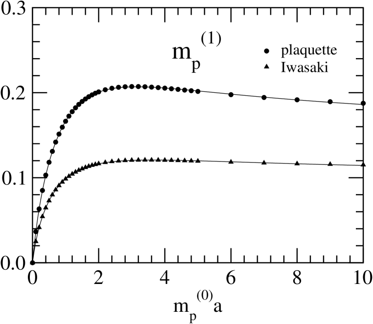
Figure 4: $m_{p}^{(1)}$ as a function of $m_{p}^{(0)}$. Solid lines denote the interpolation of $m_{p}^{(1)}$ with eq.(51)

where ${p^{*}}=(p_{0}=im_{p}^{(0)},p_{i}=0)$. It is noted that $m_{p}^{(1)}$ has no infrared divergence. In Fig. 4 we plot the $m_{p}^{(0)}$ dependence of $m_{p}^{(1)}$ for the plaquette and the Iwasaki gauge actions. We observe that $m_{p}^{(1)}$ vanishes at $m_{p}^{(0)}$=0 as expected. The solid lines denote the fitting results of the parameterization:

$$m_{p}^{(1)}=\frac{\sum_{i=1}^{3}a_{i}\{{m_{p}^{(0)}}\}^{i}}{1+\sum_{i=1}^{3}b_{i}\{{m_{p}^{(0)}}\}^{i}}.$$ (51)

The relative errors of this interpolation are less than 1% over the range $0<{m_{p}^{(0)}}\leq 10$. We tabulate the values of the parameters $a_{i}$ and $b_{i}$ ($i=1,\dots,3$) in Table 1.

The wave function $Z_{q}$ is defined as the residue of the quark propagator $S(p,m)$. The one-loop contribution on the lattice is given by

$$Z_{q}^{(1)}=\{\sinh(m_{p}^{(0)})+r_{t}\cosh(m_{p}^{(0)})\}m_{p}^{{(1)}}-{\rm Tr}\left[\frac{(\gamma_{0}+1)}{4}(-i)\frac{\partial\Sigma_{\rm latt}}{\partial p_{0}}({p^{*}},m)\right].$$ (52)

The infrared divergence in $Z_{q}^{(1)}$ is regularized by introducing the fictitious gluon mass $\lambda$. We extract the divergent term in $Z_{q}^{(1)}$ by subtracting from $I_{\Sigma}$ an analytically integrable expression ${\tilde{I}}_{\Sigma}$ which has the same infrared behavior as $I_{\Sigma}$. As a candidate of ${\tilde{I}}_{\Sigma}$ we take

$${\tilde{I}}_{\Sigma}(k,p,m_{p}^{(0)})=C_{F}Z_{q}^{(0)}\theta(\Lambda^{2}-k^{2})i\gamma_{\alpha}\frac{1}{i(p\kern-4.30554pt/+k\kern-4.30554pt/)+m_{p}^{(0)}}i\gamma_{\alpha}\frac{1}{k^{2}+\lambda^{2}}$$ (53)

with a cut-off $\Lambda$ $(\leq\pi)$. The integration is easily performedkura

$${\int_{-\pi}^{\pi}\frac{d^{4}k}{(2\pi)^{4}}}\frac{\partial{\tilde{I}}_{\Sigma}}{i\partial p\kern-4.30554pt/}(k,{p^{*}},{m_{p}^{(0)}})$$ (54)

$$= Z_{q}^{(0)}\frac{C_{F}}{16\pi^{2}}\left[-2\log\left|{\frac{\lambda^{2}}{\Lambda^{2}}}\right|-\frac{3}{4}\frac{\Lambda^{4}}{{m_{p}^{(0)}}^{4}}-\frac{9}{2}\frac{\Lambda}{{m_{p}^{(0)}}^{2}}\sqrt{\Lambda^{2}+4{m_{p}^{(0)}}^{2}}\right.$$

$$+\frac{3}{4}\frac{\Lambda}{{m_{p}^{(0)}}^{4}}(\Lambda^{2}+4{m_{p}^{(0)}}^{2})^{\frac{3}{2}}\left.-6\log\left|{\frac{\Lambda+\sqrt{\Lambda^{2}+4{m_{p}^{(0)}}^{2}}}{2{m_{p}^{(0)}}}}\right|\right],$$

It is noted that the divergent term is the same as the Wilson case in Ref. kura .

The finite renormalization factor from the lattice regularization scheme to the continuum Naive Dimensional Regularization (NDR) scheme ($\psi_{{\rm cont}}=Z_{q}^{-\frac{1}{2}}\psi_{{\rm latt}}$) is determined by

$$Z_{q} \equiv \left(Z_{q,{\rm latt}}^{(0)}\right)^{-1}\left[1-g^{2}\Delta_{q}^{(1)}({m_{p}^{(0)}})\right]=\frac{Z_{q,{\rm cont}}}{Z_{q,{\rm latt}}}$$ (55)

up to the one-loop level. Here the continuum wave function renormalization factor is given by

$$Z_{q,{\rm cont}}=1-g^{2}\frac{\partial\Sigma_{\rm cont}}{i\partial p\kern-4.30554pt/}({p^{*}},{m_{p}^{(0)}}),$$ (56)

with

$$\Sigma_{\rm cont}(p,{m_{p}^{(0)}})=C_{F}\int_{-\infty}^{\infty}\frac{d^{D}k}{(2\pi)^{D}}i\gamma_{\alpha}\frac{1}{i(p\kern-4.30554pt/+k\kern-4.30554pt/)+{m_{p}^{(0)}}}i\gamma_{\alpha}\frac{1}{k^{2}+\lambda^{2}},$$ (57)

where $D=4-2\epsilon$ ($\epsilon>0$) in the NDR scheme. The momentum assignment is depicted in Fig. 3 (a). After some algebra we obtain

$$\frac{\partial\Sigma_{\rm cont}}{i\partial p\kern-4.30554pt/}({p^{*}},{m_{p}^{(0)}})=\frac{C_{F}}{16\pi^{2}}\left[-\frac{1}{\bar{\epsilon}}-\log\left|\frac{\mu^{2}}{{{m_{p}^{(0)}}}^{2}}\right|-2\log\left|\frac{\lambda^{2}}{{{m_{p}^{(0)}}}^{2}}\right|-4\right],$$ (58)

where $1/\bar{\epsilon}=1/\epsilon-\gamma+\ln(4\pi)$ and $\mu$ is the renormalization scale. In the ${\overline{\rm MS}}$ scheme, the pole term $1/\bar{\epsilon}$ should be eliminated. From eqs.(52) and (56) the finite renormalization constant $\Delta_{q}^{(1)}({m_{p}^{(0)}})$ is expressed as

$$\Delta_{q}^{(1)}({m_{p}^{(0)}}) = \frac{\partial\Sigma_{\rm cont}}{i\partial p\kern-4.30554pt/}({p^{*}},{m_{p}^{(0)}})$$ (59)

$$\left.+\frac{\sinh({m_{p}^{(0)}})+r_{t}\cosh({m_{p}^{(0)}})}{Z_{q}^{(0)}}m_{p}^{{(1)}}-\frac{1}{Z_{q}^{(0)}}{\rm Tr}\left[\frac{(\gamma_{0}+1)}{4}(-i)\frac{\partial\Sigma_{\rm latt}}{\partial p_{0}}({p^{*}},m)\right]\right|_{\lambda=0}.$$

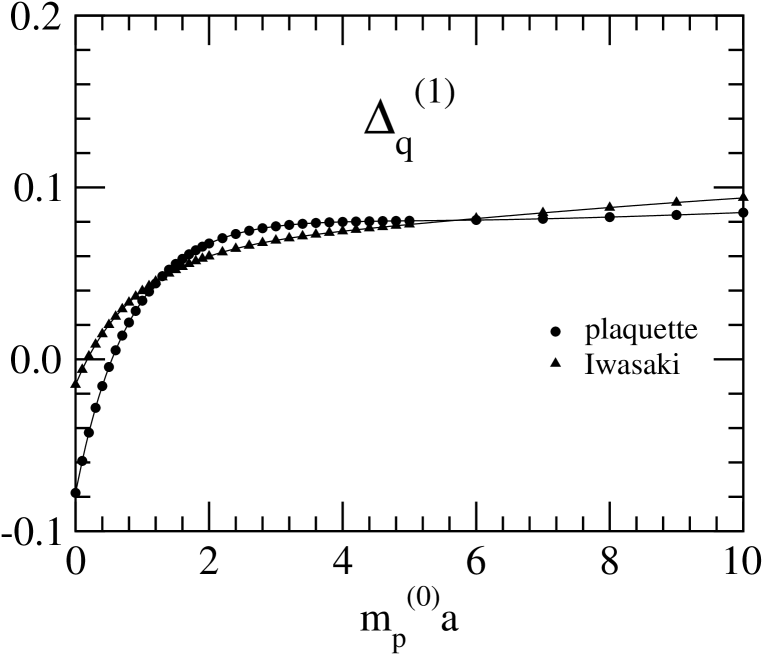
Figure 5: $\Delta_{q}^{(1)}$ as a function of $m_{p}^{(0)}$. Solid lines denote the interpolation of $\Delta_{q}^{(1)}$ with eq.(60)

Comparing eqs.(54) and (58) we find that the infrared divergence for $\lambda\rightarrow 0$ and the mass singularities at ${m_{p}^{(0)}}\rightarrow 0$ are exactly canceled out, which assures that $\Delta_{q}^{(1)}({m_{p}^{(0)}})$ is finite even in the massless limit. Figure 5 shows the ${m_{p}^{(0)}}$ dependence of $\Delta_{q}^{(1)}({m_{p}^{(0)}})$ for the plaquette and the Iwasaki gauge actions. We parameterize $\Delta_{q}^{(1)}$ as

$$\Delta_{q}^{(1)}=\Delta_{q}^{(1)}({m_{p}^{(0)}}=0)+\frac{\sum_{i=1}^{4}a_{i}\{{m_{p}^{(0)}}\}^{i}}{1+\sum_{i=1}^{4}b_{i}\{{m_{p}^{(0)}}\}^{i}},$$ (60)

where the values of $\Delta_{q}^{(1)}({m_{p}^{(0)}}=0)$ except for the DBW2 gauge action are taken from Ref. gmass . The fitting results are drawn in Fig. 5 by solid lines, whose relative errors are at most 1% over the range $0<{m_{p}^{(0)}}\leq 10$. The values of the parameters $a_{i}$, $b_{i}$ ($i=1,\dots,4$) and $\Delta_{q}^{(1)}({m_{p}^{(0)}}=0)$ are listed in Table 2.

The parameter $\nu$ is determined by adjusting the speed of light in $S^{-1}(p,m)$. Comparing the coefficients of $\gamma_{0}$ and $\gamma_{i}$ in the numerator we obtain

$$\nu=\frac{\sinh(m_{p})}{m_{p}}\frac{[1-g^{2}B_{0}({p^{*}},m)]}{[1-g^{2}B_{i}({p^{*}},m)]}.$$ (61)

The one-loop contribution is given by

$$\nu^{(1)}=\left(\frac{\cosh({m_{p}^{(0)}})}{{m_{p}^{(0)}}}-\frac{\sinh({m_{p}^{(0)}})}{({m_{p}^{(0)}})^{2}}\right)m_{p}^{(1)}+\nu^{(0)}\{B_{i}({p^{*}},m)-B_{0}({p^{*}},m)\},$$ (62)

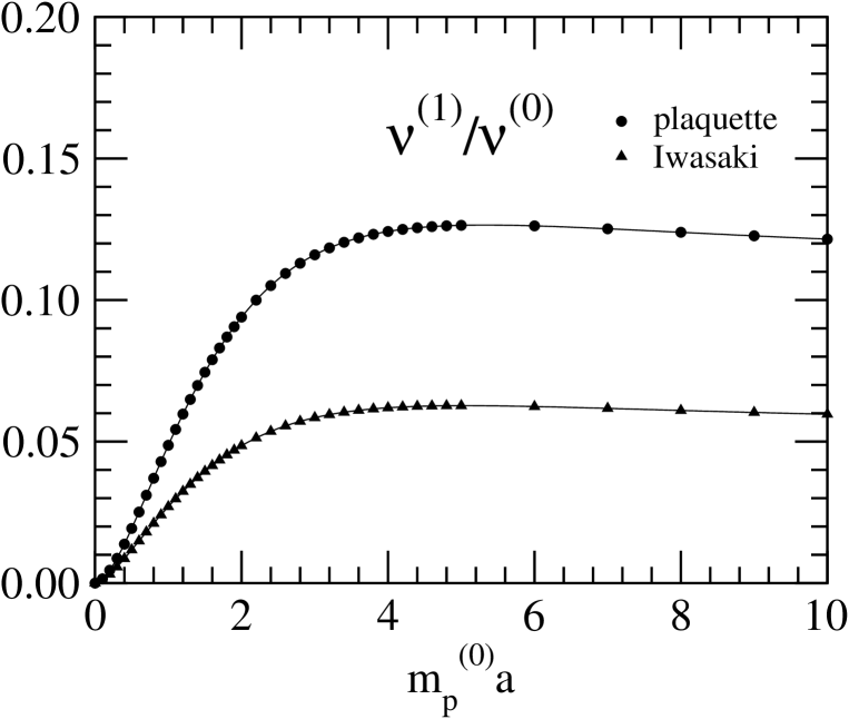
Figure 6: $\nu^{(1)}/\nu^{(0)}$ as a function of $m_{p}^{(0)}$. Solid lines denote the interpolation of $\nu^{(1)}/\nu^{(0)}$ with eq.(63)

where $B_{i}$ and $B_{0}$ have no infrared divergence. The quark mass dependences of $\nu^{(1)}/\nu^{(0)}$ for the plaquette and the Iwasaki gauge actions are shown in Fig. 6. As expected $\nu^{(1)}$ vanishes at $m_{p}^{(0)}=0$ for both cases. The solid lines depict the results of the interpolation:

$$\frac{\nu^{(1)}}{\nu^{(0)}}=\frac{\sum_{i=1}^{5}a_{i}\{{m_{p}^{(0)}}\}^{i}}{1+\sum_{i=1}^{5}b_{i}\{{m_{p}^{(0)}}\}^{i}}.$$ (63)

The relative errors of this interpolation are less than a few % over the range $0<{m_{p}^{(0)}}\leq 10$. The values of the parameters $a_{i}$ and $b_{i}$ ($i=1,\dots,5$) are collected in Table 3.

The parameter $r_{s}$ is determined from $S^{-1}(p,m)$ such that the correct dispersion relation is reproduced:

$$E^{2}=m_{p}^{2}+\sum_{i}p_{i}^{2}+O(p_{i}^{4}).$$ (64)

This condition yields

$$r_{s}^{(1)} = \frac{1}{m_{p}^{(0)}}\{Z_{q}^{(1)}+\nu^{(0)}B_{i}({p^{*}},m)-\nu^{(1)}\}-\frac{m_{p}^{(1)}}{m_{p}^{(0)}}r_{s}^{(0)}+{\rm Tr}\left[\frac{(1+\gamma_{0})}{2}\frac{\partial\Sigma}{\partial p_{k}^{2}}({p^{*}},m)\right].$$ (65)

The infrared divergence of the last term can be extracted by using ${\tilde{I}}_{\Sigma}$ in eq.(53):

$${\int_{-\pi}^{\pi}\frac{d^{4}k}{(2\pi)^{4}}}\frac{\partial{\tilde{I}}_{\Sigma}}{\partial p_{k}^{2}}(k,{p^{*}},{m_{p}^{(0)}})$$ (66)

$$= \frac{Z_{q}^{(0)}}{{m_{p}^{(0)}}}\frac{C_{F}}{16\pi^{2}}\left[\log\left|\frac{\Lambda^{2}}{\lambda^{2}}\right|-\frac{\Lambda^{2}}{{m_{p}^{(0)}}^{2}}-\frac{1}{2}\frac{\Lambda^{4}}{{m_{p}^{(0)}}^{4}}-2\frac{\Lambda}{{m_{p}^{(0)}}^{2}}\sqrt{\Lambda^{2}+4{m_{p}^{(0)}}^{2}}\right.$$

$$+\frac{1}{2}\frac{\Lambda}{{m_{p}^{(0)}}^{4}}(\Lambda^{2}+4{m_{p}^{(0)}}^{2})^{\frac{3}{2}}\left.-2\log\left|{\frac{\Lambda+\sqrt{\Lambda^{2}+4{m_{p}^{(0)}}^{2}}}{2{m_{p}^{(0)}}}}\right|\right].$$

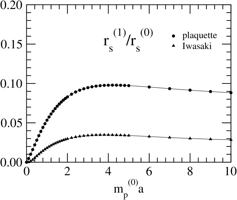
Figure 7: $r_{s}^{(1)}/r_{s}^{(0)}$ as a function of $m_{p}^{(0)}$. Solid lines denote the interpolation of $r_{s}^{(1)}/r_{s}^{(0)}$ with eq.(67)

We find that the infrared divergence and the mass singularity in the last term are exactly canceled out by those in $Z_{q}^{(1)}/{{m_{p}^{(0)}}}$. We show the ${m_{p}^{(0)}}$ dependence of $r_{s}^{(1)}/r_{s}^{(0)}$ for the plaquette and the Iwasaki gauge actions in Fig. 7, where $r_{s}^{(1)}/r_{s}^{(0)}$ becomes close to zero as ${m_{p}^{(0)}}$ vanishes. This is an expected behavior because the deviation of $r_{s}$ from $r_{t}$ stems from the power corrections of ${m_{p}^{(0)}}a$. The quark mass dependence of $r_{s}^{(1)}/r_{s}^{(0)}$ is well described by the interpolation with the relative errors of less than a few % over the range $0<{m_{p}^{(0)}}\leq 10$,

$$\frac{r_{s}^{(1)}}{r_{s}^{(0)}}=\frac{\sum_{i=1}^{5}a_{i}\{{m_{p}^{(0)}}\}^{i}}{1+\sum_{i=1}^{5}b_{i}\{{m_{p}^{(0)}}\}^{i}}.$$ (67)

We give the values of the parameters $a_{i}$ and $b_{i}$ ($i=1,\dots,5$) in Table 4.

V Determination of ${\it c}_{\it E}$ and ${\it c}_{\it B}$ up to the one-loop level

We employ the on-shell quark-quark scattering amplitude to determine ${\it c}_{\it E}$ and ${\it c}_{\it B}$. At the tree level the parameters $\nu$, $r_{s}$, ${\it c}_{\it E}$ and ${\it c}_{\it B}$ are adjusted to reproduce the continuum form of the scattering amplitude at the on-shell point removing the $m_{Q}a$ correctionsakt ,

$$T = -g^{2}(T^{A})^{2}{\bar{u}}(p^{\prime})\gamma_{\mu}u(p)D_{\mu\nu}(p-p^{\prime}){\bar{u}}(q^{\prime})\gamma_{\nu}u(q)$$ (68)

$$-g^{2}(T^{A})^{2}{\bar{u}}(q^{\prime})\gamma_{\mu}u(p)D_{\mu\nu}(p-q^{\prime}){\bar{u}}(p^{\prime})\gamma_{\nu}u(q)$$

$$+O((p_{i}a)^{2},(q_{i}a)^{2},(p^{\prime}_{i}a)^{2},(q_{i}^{\prime}a)^{2}),$$

where the momentum assignment is depicted in Fig. 8 and $D_{\mu\nu}$ denotes the gluon propagator. At the tree level the quark-quark-gluon vertex is written as

$$\left({\bar{u}}(p^{\prime})\Lambda_{0}^{(0)}(p,p^{\prime})u(p)\right)_{\rm latt} = Z_{q}^{(0)}\left({\bar{u}}(p^{\prime})i\gamma_{0}u(p)\right)_{\rm cont}+O((p_{i}a)^{2},(p_{i}^{\prime}a)^{2}),$$ (69)

$$\left({\bar{u}}(p^{\prime})\Lambda_{k}^{(0)}(p,p^{\prime})u(p)\right)_{\rm latt} = Z_{q}^{(0)}\left({\bar{u}}(p^{\prime})i\gamma_{k}u(p)\right)_{\rm cont}+O((p_{i}a)^{2},(p_{i}^{\prime}a)^{2}),$$ (70)

for

$$\Lambda_{0}^{(0)}(p,p^{\prime}) = i\gamma_{0}\cos\left(\frac{p_{0}+p^{\prime}_{0}}{2}\right)\ +r_{t}\sin\left(\frac{p_{0}+p^{\prime}_{0}}{2}\right)$$ (71)

$$+\frac{{\it c}_{\it E}^{(0)}}{2}\cos\left(\frac{p_{0}-p^{\prime}_{0}}{2}\right)\sum_{l}\sigma_{0l}\sin(p_{l}-p^{\prime}_{l}),$$

$$\Lambda_{k}^{(0)}(p,p^{\prime}) = i\nu^{(0)}\gamma_{k}\cos\left(\frac{p_{k}+p^{\prime}_{k}}{2}\right)\ +r_{s}^{(0)}\sin\left(\frac{p_{k}+p^{\prime}_{k}}{2}\right)$$ (72)

$$+\frac{{\it c}_{\it E}^{(0)}}{2}\cos\left(\frac{p_{k}-p^{\prime}_{k}}{2}\right)\sigma_{k0}\sin(p_{0}-p^{\prime}_{0})$$

$$+\frac{{\it c}_{\it B}^{(0)}}{2}\cos\left(\frac{p_{k}-p^{\prime}_{k}}{2}\right)\sum_{l\neq k}\sigma_{kl}\sin(p_{l}-p^{\prime}_{l}),$$

where the spinor on the lattice is given by

$$u(p)=\left(\begin{array}[]{c}\phi\\ \frac{\nu{\vec{p}}\cdot{\vec{\sigma}}}{N(p)}\phi\end{array}\right)+O((p_{i}a)^{2}),$$ (73)

with $N(p)=(-i){\rm sin}(p_{0})+m_{0}+r_{t}(1-{\rm cos}(p_{0}))+r_{s}\sum_{i}(1-{\rm cos}(p_{i}))$. The $O(a)$ improvement condition yields

$$\nu^{(0)} = \frac{\sinh({m_{p}^{(0)}})}{{m_{p}^{(0)}}},$$ (74)

$$r_{s}^{(0)} = \frac{\cosh({m_{p}^{(0)}})+r_{t}\sinh({m_{p}^{(0)}})}{{m_{p}^{(0)}}}-\frac{\sinh({m_{p}^{(0)}})}{{m_{p}^{(0)}}^{2}},$$ (75)

$${\it c}_{\it E}^{(0)} = r_{t}\nu^{(0)},$$ (76)

$${\it c}_{\it B}^{(0)} = r_{s}^{(0)}.$$ (77)

It should be noted that the values of $\nu^{(0)}$ and $r_{s}^{(0)}$ are exactly the same as those determined from the quark propagator.

Let us turn to the one-loop calculation. Recently the authors have shown the validity of the conventional perturbative method to determine the clover coefficient ${c_{\rm SW}}$ up to the one-loop level in the massless case from the on-shell quark-quark scattering amplitudecsw_m0 . We extend this calculation to the massive case. According to Ref. csw_m0 , it is sufficient for us to improve each on-shell quark-quark-gluon vertex individually. To determine the one-loop coefficients ${\it c}_{\it E}^{(1)}$ and ${\it c}_{\it B}^{(1)}$ we need six types of diagrams shown in Fig. 9. We first consider to calculate ${\it c}_{\it B}^{(1)}$. Without the space-time symmetry the general form of the off-shell vertex function at the one-loop level is written as

$$\Lambda_{k}^{(1)}(p,q,m) = \sum_{i=a,\dots,f}\Lambda_{k}^{(1-i)}(p,q,m)$$ (78)

$$= \sum_{i=a,\dots,f}\int_{-\pi}^{\pi}\frac{d^{4}k}{(2\pi)^{4}}I_{k}^{(i)}(k,p,q,m)$$

$$= \gamma_{k}F_{1}^{k}+\gamma_{k}\{p\kern-4.30554pt/F_{2}^{k}+p\kern-4.30554pt/_{0}F_{3}^{k}\}+\{q\kern-4.30554pt/F_{4}^{k}+q\kern-4.30554pt/_{0}F_{5}^{k}\}\gamma_{k}$$

$$+q\kern-4.30554pt/\gamma_{k}p\kern-4.30554pt/F_{6}^{k}+q\kern-4.30554pt/\gamma_{k}p\kern-4.30554pt/_{0}F_{7}^{k}+q\kern-4.30554pt/_{0}\gamma_{k}p\kern-4.30554pt/F_{8}^{k}$$

$$+(p_{k}+q_{k})\left[H_{1}^{k}+p\kern-4.30554pt/H_{2}^{k}+q\kern-4.30554pt/H_{3}^{k}+q\kern-4.30554pt/p\kern-4.30554pt/H_{4}^{k}\right]$$

$$+(p_{k}-q_{k})\left[G_{1}^{k}+p\kern-4.30554pt/G_{2}^{k}+q\kern-4.30554pt/G_{3}^{k}+q\kern-4.30554pt/p\kern-4.30554pt/G_{4}^{k}\right]+O(a^{2}),$$

where $\Lambda_{k}(p,q,m)=\Lambda_{k}^{(0)}(p,q,m)+g^{2}\Lambda_{k}^{(1)}(p,q,m)+O(g^{4})$ and

$$p\kern-4.30554pt/ = \sum_{\alpha=0}^{3}p_{\alpha}\gamma_{\alpha},$$ (79)

$$q\kern-4.30554pt/ = \sum_{\alpha=0}^{3}q_{\alpha}\gamma_{\alpha},$$ (80)

$$p\kern-4.30554pt/_{0} = p_{0}\gamma_{0},$$ (81)

$$q\kern-4.30554pt/_{0} = q_{0}\gamma_{0}.$$ (82)

The coefficients $F_{i}^{k}$ ($i=1,\dots,8$), $G_{i}^{k}$ ($i=1,2,3,4$) and $H_{i}^{k}$ ($i=1,2,3,4$) are functions of $p^{2}$, $q^{2}$, $p\cdot q$ and $m$. From the charge conjugation symmetry they have to satisfy the following condition:

$$F_{2}^{k}=F_{4}^{k},$$ (83)

$$F_{3}^{k}=F_{5}^{k},$$ (84)

$$F_{7}^{k}=F_{8}^{k},$$ (85)

$$H_{2}^{k}=H_{3}^{k},$$ (86)

$$G_{1}^{k}=G_{4}^{k}=0,$$ (87)

$$G_{2}^{k}=-G_{3}^{k}.$$ (88)

Sandwiching $\Lambda_{k}^{(1)}(p,q,m)$ by the on-shell quark states $u(p)$ and $\bar{u}(q)$, which satisfy $p\kern-4.30554pt/u(p)=im_{p}u(p)$ and $\bar{u}(q)q\kern-4.30554pt/=im_{p}\bar{u}(q)$, the matrix element is reduced to

$${\bar{u}}(q)\Lambda_{k}^{(1)}(p,q,m)u(p)$$ (89)

$$= {\bar{u}}(q)\gamma_{k}u(p)\left\{F_{1}^{k}+im_{p}(F_{2}^{k}+F_{4}^{k})-m_{p}^{2}F_{6}^{k}\right\}$$

$$+{\bar{u}}(q)\gamma_{k}\gamma_{0}u(p)(p_{0}-q_{0})\left\{F_{3}^{k}+im_{p}F_{7}^{k}\right\}$$

$$+(p_{k}+q_{k}){\bar{u}}(q)u(p)\left\{H_{1}^{k}+im_{p}(H_{2}^{k}+H_{3}^{k})-m_{p}^{2}H_{4}^{k}\right\}$$

$$+(p_{k}-q_{k}){\bar{u}}(q)u(p)\left\{G_{1}^{k}+im_{p}(G_{2}^{k}+G_{3}^{k})-m_{p}^{2}G_{4}^{k}\right\}+O(a^{2}),$$

where we use $F_{3}^{k}=F_{5}^{k}$ and $F_{7}^{k}=F_{8}^{k}$. (Note that we can replace $m_{p}$ with ${m_{p}^{(0)}}$ in the 1-loop diagrams.) The first term in the right hand side contributes to the renormalization factor of the quark-quark-gluon vertex, which is equal to $Z_{q}^{(0)}$ at the tree level. From eqs.(87) and (88) we find that the last term of eq.(89) vanishes: this term is not allowed from the charge conjugation symmetry. It is also possible to numerically check $G_{1}^{k}+im_{p}(G_{2}^{k}+G_{3}^{k})-m_{p}^{2}G_{4}^{k}=0$.

The contribution of the second term is $O(a^{2})$. This can be shown as follows. For simplicity we first consider the case of ${\Lambda}_{\rm QCD}\ll m_{Q}\ll a^{-1}$. The difference of $p_{0}$ and $q_{0}$ is expressed as

$$(p_{0}-q_{0})a = \left(\sqrt{m_{p}^{2}+p_{i}^{2}}-\sqrt{m_{p}^{2}+q_{i}^{2}}\right)a$$ (90)

$$= \left(\frac{p_{i}^{2}-q_{i}^{2}}{m_{p}}\right)a+O\left(\frac{p_{i}^{4}}{m_{p}^{3}}a,\frac{q_{i}^{4}}{m_{p}^{3}}a\right).$$

Since the terms $\gamma_{k}p\kern-4.30554pt/_{0}$, $q\kern-4.30554pt/_{0}\gamma_{k}$, $q\kern-4.30554pt/\gamma_{k}p\kern-4.30554pt/_{0}$ and $q\kern-4.30554pt/_{0}\gamma_{k}p\kern-4.30554pt/$ represent the violation of the Lorentz symmetry due to the finite $m_{Q}a$ corrections, their coefficients should vanish at the massless limit, namely $F_{3}^{k}$, $F_{7}^{k}$ $\propto$ $m_{p}a$ as their leading contributions. Hence the combination of $F_{3}^{k}$, $F_{7}^{k}$ and $(p_{0}-q_{0})a$ results in $O(a^{2})$. This is retained even in the case of ${\Lambda}_{\rm QCD}\ll m_{Q}\sim a^{-1}$.

The relevant term for the determination of ${\it c}_{\it B}$ is the third one, which can be extracted by setting $p={p^{*}}\equiv(p_{0}=im_{p},p_{i}=0)$ and $q={q^{*}}\equiv(q_{0}=im_{p},q_{i}=0)$ in eq.(78):

$$\left.H_{1}^{k}+im_{p}(H_{2}^{k}+H_{3}^{k})-m_{p}^{2}H_{4}^{k}\right|_{p={p^{*}},q={q^{*}}}$$ (91)

$$= \frac{1}{8}{\rm Tr}\left[\left\{\frac{\partial}{\partial p_{k}}+\frac{\partial}{\partial q_{k}}\right\}\Lambda_{k}^{(1)}({p^{*}},{q^{*}},m)(\gamma_{4}+1)\right]$$

$$-\frac{1}{8}{\rm Tr}\left[\left\{\frac{\partial}{\partial p_{i}}-\frac{\partial}{\partial q_{i}}\right\}\Lambda_{k}^{(1)}({p^{*}},{q^{*}},m)(\gamma_{4}+1)\gamma_{i}\gamma_{k}\right]^{i\neq k},$$

where we have used the fact that $F^{k}$, $G^{k}$ and $H^{k}$ are functions of $p^{2}$, $q^{2}$ and $p\cdot q$, so that

$$\left.\frac{\partial F_{j}^{k}}{\partial p_{i}}\right|_{p={p^{*}},q={q^{*}}}=\left.\frac{\partial F_{j}^{k}}{\partial q_{i}}\right|_{p={p^{*}},q={q^{*}}}=0,$$ (92)

$$\left.\frac{\partial H_{l}^{k}}{\partial p_{i}}\right|_{p={p^{*}},q={q^{*}}}=\left.\frac{\partial H_{l}^{k}}{\partial q_{i}}\right|_{p={p^{*}},q={q^{*}}}=0,$$ (93)

$$\left.\frac{\partial G_{l}^{k}}{\partial p_{i}}\right|_{p={p^{*}},q={q^{*}}}=\left.\frac{\partial G_{l}^{k}}{\partial q_{i}}\right|_{p={p^{*}},q={q^{*}}}=0$$ (94)

with $j=1,\dots,8$, $l=1,2,3,4$ and $i=1,2,3$.

We should remark that the third term in eq.(89) contains both the lattice artifact of $O(p_{k}a,q_{k}a)$ and the physical contribution of $O(p_{k}/m,q_{k}/m)$. The parameter ${\it c}_{\it B}$ is determined to eliminate the lattice artifacts of $O(p_{k}a,q_{k}a)$:

$$\frac{{\it c}_{\it B}^{(1)}-r_{s}^{(1)}}{2} = \left[H_{1}^{k}+im_{p}(H_{2}^{k}+H_{3}^{k})-m_{p}^{2}H_{4}^{k}\right]_{p={p^{*}},q={q^{*}}}^{\rm latt}$$ (95)

$$-Z_{q}^{(0)}\left[H_{1}^{k}+im_{p}(H_{2}^{k}+H_{3}^{k})-m_{p}^{2}H_{4}^{k}\right]_{p={p^{*}},q={q^{*}}}^{\rm cont},$$

where we take account of the tree level expression for the quark-quark-gluon vertex in eq.(70) and eq.(3.51) in Ref. akt .

We first show the calculation of eq.(91) in the continuum theory. The contributions of Figs. 9 (a) and (b) are expressed as

$$\Lambda_{k,{\rm cont}}^{(1-a,b)}(p,q,m) = \int_{-\infty}^{\infty}\frac{d^{D}k}{(2\pi)^{D}}I_{k,{\rm cont}}^{(a,b)}(k,p,q,m)$$ (96)

with

$$I_{k,{\rm cont}}^{(a)}(k,p,q,m) = \left(-\frac{1}{2N_{c}}\right)i\gamma_{\alpha}\frac{1}{i(q\kern-4.30554pt/+k\kern-4.30554pt/)+{m_{p}^{(0)}}}i\gamma_{k}\frac{1}{i(p\kern-4.30554pt/+k\kern-4.30554pt/)+{m_{p}^{(0)}}}i\gamma_{\alpha}\frac{1}{k^{2}+\lambda^{2}},$$ (97)

$$I_{k,{\rm cont}}^{(b)}(k,p,q,m) = \left(-\frac{N_{c}}{2}\right)i\gamma_{\beta}\frac{1}{i(q\kern-4.30554pt/-k\kern-4.30554pt/)+{m_{p}^{(0)}}}i\gamma_{\alpha}\frac{1}{k^{2}+\lambda^{2}}\frac{1}{(p-q+k)^{2}+\lambda^{2}}$$

$$\times\left[\delta_{\alpha\beta}(-p_{k}+q_{k}-2k_{k})+\delta_{k\beta}(-p_{\alpha}+q_{\alpha}+k_{\alpha})+\delta_{k\alpha}(2p_{\beta}-2q_{\beta}+k_{\beta})\right],$$

where we have replaced $m_{p}$ with ${m_{p}^{(0)}}$ in the 1-loop diagrams. Note that Figs. 9 (c), (d), (e) and (f) do not exist in the continuum. Applying the formula of eq.(91) we obtain

$$(a) : \left(-\frac{1}{2N_{c}}\right)\frac{-1}{16\pi^{2}}\frac{1}{{m_{p}^{(0)}}},$$ (99)

$$(b) : \left(-\frac{N_{c}}{2}\right)\frac{1}{16\pi^{2}}\frac{1}{{m_{p}^{(0)}}}\left[-\log\left|\frac{{m_{p}^{(0)}}^{2}}{\lambda^{2}}\right|+3\right].$$ (100)

Here it should be remarked that we find the same results for the time component of the vertex function because of the space-time symmetry in the continuum theory.

To investigate the infrared behavior of the lattice integrand $I_{k,{\rm latt}}^{(1)}(k,p,q,m)$ we expand it in terms of $k$. The following terms possibly yield logarithmic divergences:

$$(a) : \left(-\frac{1}{2N_{c}}\right)2{m_{p}^{(0)}}^{2}({\it c}_{\it B}^{(0)}-r_{s}^{(0)})J_{a}(k,{m_{p}^{(0)}},\lambda),$$ (101)

$$(b) : \left(-\frac{N_{c}}{2}\right)\left[-{m_{p}^{(0)}}({\it c}_{\it B}^{(0)}+2r_{s}^{(0)})J_{b}(k,{m_{p}^{(0)}},\lambda)\right.$$ (102)

$$\left.+{4Z_{q}^{(0)}}\left\{J_{b}(k,{m_{p}^{(0)}},\lambda)+{m_{p}^{(0)}}J_{c}(k,{m_{p}^{(0)}},\lambda)\right\}\right],$$

$$(c) : \left(-\frac{N_{c}}{4}\right)(-3){\it c}_{\it B}^{(0)}J_{d}(k,\lambda),$$ (103)

where

$$J_{a}(k,{m_{p}^{(0)}},\lambda) = \frac{1}{k^{2}+\lambda^{2}}\frac{1}{(k^{2}+2i{m_{p}^{(0)}}k_{4})^{2}},$$ (104)

$$J_{b}(k,{m_{p}^{(0)}},\lambda) = \frac{1}{(k^{2}+\lambda^{2})^{2}}\frac{ik_{4}}{k^{2}-2i{m_{p}^{(0)}}k_{4}},$$ (105)

$$J_{c}(k,{m_{p}^{(0)}},\lambda) = \frac{1}{(k^{2}+\lambda^{2})^{2}}\frac{k_{i}^{2}}{(k^{2}-2i{m_{p}^{(0)}}k_{4})^{2}},$$ (106)

$$J_{d}(k,\lambda) = \frac{1}{(k^{2}+\lambda^{2})^{2}}$$ (107)

with no sum for the index $i$. Figures 9 (d), (e) and (f) have no infrared divergence as long as $m\not=0$. The coefficients of the logarithmic divergence for $J_{i}$ ($i=a,b,c,d$) are obtained by performing the integration with the cutoff $\Lambda$:

$${\int_{-\pi}^{\pi}\frac{d^{4}k}{(2\pi)^{4}}}\theta(\Lambda^{2}-k^{2})J_{a}(k,{m_{p}^{(0)}},\lambda) = \frac{1}{16\pi^{2}}\frac{1}{{m_{p}^{(0)}}^{2}}\left[\frac{1}{2}\log\left|\frac{\Lambda^{2}}{\lambda^{2}}\right|\right.$$ (108)

$$\left.-\log\left|{\frac{\Lambda+\sqrt{\Lambda^{2}+4{m_{p}^{(0)}}^{2}}}{2{m_{p}^{(0)}}}}\right|\right],$$

$${\int_{-\pi}^{\pi}\frac{d^{4}k}{(2\pi)^{4}}}\theta(\Lambda^{2}-k^{2})J_{b}(k,{m_{p}^{(0)}},\lambda) = \frac{1}{16\pi^{2}}\frac{1}{{m_{p}^{(0)}}}\left[-\frac{1}{2}\log\left|\frac{\Lambda^{2}}{\lambda^{2}}\right|+\frac{1}{2}-\frac{1}{4}\frac{\Lambda^{2}}{{m_{p}^{(0)}}^{2}}\right.$$

$$\left.+\frac{1}{4}\frac{\Lambda}{{m_{p}^{(0)}}^{2}}\sqrt{\Lambda^{2}+4{m_{p}^{(0)}}^{2}}+\log\left|{\frac{\Lambda+\sqrt{\Lambda^{2}+4{m_{p}^{(0)}}^{2}}}{2{m_{p}^{(0)}}}}\right|\right],$$

$${\int_{-\pi}^{\pi}\frac{d^{4}k}{(2\pi)^{4}}}\theta(\Lambda^{2}-k^{2})J_{c}(k,{m_{p}^{(0)}},\lambda) = -\frac{1}{2{m_{p}^{(0)}}}{\int_{-\pi}^{\pi}\frac{d^{4}k}{(2\pi)^{4}}}\theta(\Lambda^{2}-k^{2})J_{b}(k,{m_{p}^{(0)}},\lambda),$$ (110)

$${\int_{-\pi}^{\pi}\frac{d^{4}k}{(2\pi)^{4}}}\theta(\Lambda^{2}-k^{2})J_{d}(k,\lambda) = \frac{1}{16\pi^{2}}\left[\log\left|\frac{\Lambda^{2}}{\lambda^{2}}\right|-1\right].$$ (111)

From these results we find the coefficients of the infrared divergence in Figs. 9 (a), (b) and (c):

$$(a) : \left(-\frac{1}{2N_{c}}\right)({\it c}_{\it B}^{(0)}-r_{s}^{(0)})L,$$ (112)

$$(b) : \left(-\frac{N_{c}}{2}\right)\left[\frac{{\it c}_{\it B}^{(0)}+2r_{s}^{(0)}}{2}L-\frac{Z_{q}^{(0)}}{{m_{p}^{(0)}}}L\right],$$ (113)

$$(c) : \left(-\frac{N_{c}}{4}\right)(-3){\it c}_{\it B}^{(0)}L,$$ (114)

where

$$L=\frac{1}{16\pi^{2}}\ln\left|\frac{\Lambda^{2}}{\lambda^{2}}\right|.$$ (115)

Taking the summation the total contribution is

$$\left(-\frac{1}{2N_{c}}+\frac{N_{c}}{2}\right)({\it c}_{\it B}^{(0)}-r_{s}^{(0)})L-\left(-\frac{N_{c}}{2}\right)\frac{Z_{q}^{(0)}}{{m_{p}^{(0)}}}L.$$ (116)

If the tree level values are properly tuned as ${\it c}_{\it B}^{(0)}=r_{s}^{(0)}$, we are left with $-(-N_{c}/2)({Z_{q}^{(0)}}/{{m_{p}^{(0)}}})L$, which is exactly the same as the infrared divergence in the continuum theory with the correct normalization factor.

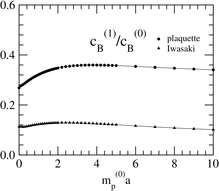
Figure 10: ${\it c}_{\it B}^{(1)}/{\it c}_{\it B}^{(0)}$ as a function of $m_{p}^{(0)}$. Solid lines denote the interpolation of ${\it c}_{\it B}^{(1)}/{\it c}_{\it B}^{(0)}$ with eq.(117)

Figure 10 shows the quark mass dependences of ${\it c}_{\it B}^{(1)}/{\it c}_{\it B}^{(0)}$ for the plaquette and the Iwasaki gauge actions. We find relatively modest quark mass dependences for both cases. The solid lines denote the fitting results of the interpolation:

$$\frac{{\it c}_{\it B}^{(1)}}{{\it c}_{\it B}^{(0)}}=\left.\frac{{\it c}_{\it B}^{(1)}}{{\it c}_{\it B}^{(0)}}\right|_{{m_{p}^{(0)}}=0}+\frac{\sum_{i=1}^{5}a_{i}\{{m_{p}^{(0)}}\}^{i}}{1+\sum_{i=1}^{5}b_{i}\{{m_{p}^{(0)}}\}^{i}},$$ (117)

where the values of the parameters $a_{i}$ and $b_{i}$ ($i=1,\dots,5$) are given in Table 3 together with ${\it c}_{\it B}^{(1)}/{\it c}_{\it B}^{(0)}$ at ${m_{p}^{(0)}}=0$ taken from Ref. csw_m0 . The relative errors of this interpolation are less than a few % over the range $0<{m_{p}^{(0)}}\leq 10$.

We now turn to the calculation of ${\it c}_{\it E}^{(1)}$. The general form of the off-shell vertex function for the time component at the one-loop level is written as

$$\Lambda_{0}^{(1)}(p,q,m) = \sum_{i=a,\dots,f}\Lambda_{0}^{(1-i)}(p,q,m)$$ (118)

$$= \sum_{i=a,\dots,f}\int_{-\pi}^{\pi}\frac{d^{4}k}{(2\pi)^{4}}I_{0}^{(i)}(k,p,q,m)$$

$$= \gamma_{0}F_{1}^{0}+\gamma_{0}p\kern-4.30554pt/F_{2}^{0}+q\kern-4.30554pt/\gamma_{0}F_{3}^{0}+q\kern-4.30554pt/\gamma_{0}p\kern-4.30554pt/F_{4}^{0}$$

$$+(p_{0}+q_{0})\left[H_{1}^{0}+p\kern-4.30554pt/H_{2}^{0}+q\kern-4.30554pt/H_{3}^{0}+q\kern-4.30554pt/p\kern-4.30554pt/H_{4}^{0}\right]$$

$$+(p_{0}-q_{0})\left[G_{1}^{0}+p\kern-4.30554pt/G_{2}^{0}+q\kern-4.30554pt/G_{3}^{0}+q\kern-4.30554pt/p\kern-4.30554pt/G_{4}^{0}\right]+O(a^{2}),$$

where we define $\Lambda_{0}(p,q,m)=\Lambda_{0}^{(0)}(p,q,m)+g^{2}\Lambda_{0}^{(1)}(p,q,m)+O(g^{4})$. The coefficients $F_{i}^{0}$, $G_{i}^{0}$ and $H_{i}^{0}$ ($i=1,2,3,4$) are functions of $p^{2}$, $q^{2}$, $p\cdot q$ and $m$. As in the case of $\Lambda_{k}$ the charge conjugation symmetry provides the coefficients with the following constraint:

$$F_{2}^{0}=F_{3}^{0},$$ (119)

$$H_{2}^{0}=H_{3}^{0},$$ (120)

$$G_{1}^{0}=G_{4}^{0}=0,$$ (121)

$$G_{2}^{0}=-G_{3}^{0}.$$ (122)

Sandwiching $\Lambda_{0}^{(1)}(p,q,m)$ by the on-shell quark states as before, the matrix element is reduced to

$${\bar{u}}(q)\Lambda_{0}^{(1)}(p,q,m)u(p)$$ (123)

$$= {\bar{u}}(q)\gamma_{0}u(p)\left\{F_{1}^{0}+i{m_{p}^{(0)}}(F_{2}^{0}+F_{3}^{0})-{m_{p}^{(0)}}^{2}F_{4}^{0}\right\}$$

$$+(p_{0}+q_{0}){\bar{u}}(q)u(p)\left\{H_{1}^{0}+i{m_{p}^{(0)}}(H_{2}^{0}+H_{3}^{0})-{m_{p}^{(0)}}^{2}H_{4}^{0}\right\}$$

$$+(p_{0}-q_{0}){\bar{u}}(q)u(p)\left\{G_{1}^{0}+i{m_{p}^{(0)}}(G_{2}^{0}+G_{3}^{0})-{m_{p}^{(0)}}^{2}G_{4}^{0}\right\}+O(a^{2}).$$

Here we replace $m_{p}$ with ${m_{p}^{(0)}}$. The renormalization factor is determined from the combination of $F_{1}^{0}+i{m_{p}^{(0)}}(F_{2}^{0}+F_{3}^{0})-{m_{p}^{(0)}}^{2}F_{4}^{0}$, which should be the same as $F_{1}^{k}+i{m_{p}^{(0)}}(F_{2}^{k}+F_{4}^{k})-{m_{p}^{(0)}}^{2}F_{6}^{k}$ in eq.(89). The last term of eq.(123) vanishes from eqs.(121) and (122) as a consequence of the charge conjugation symmetry. We can also check $G_{1}^{0}+i{m_{p}^{(0)}}(G_{2}^{0}+G_{3}^{0})-{m_{p}^{(0)}}^{2}G_{4}^{0}=0$ numerically.

The coefficient ${\it c}_{\it E}$ is determined to remove the $O(a)$ contribution of the second term in the right hand side, where the physical contribution of $O(p_{0}/m,q_{0}/m)$ is also included. The second term is extracted by setting $p={p^{*}}$ and $q={q^{*}}$ in eq.(118) as

$$\left.H_{1}^{0}+i{m_{p}^{(0)}}(H_{2}^{0}+H_{3}^{0})-{m_{p}^{(0)}}^{2}H_{4}^{0}\right|_{p={p^{*}},q={q^{*}}}$$ (124)

$$= \frac{1}{8}{\rm Tr}\left[\left\{\frac{\partial}{\partial p_{i}}+\frac{\partial}{\partial q_{i}}\right\}\Lambda_{0}^{(1)}({p^{*}},{q^{*}},m)\gamma_{i}\right]$$

$$+\frac{1}{i{m_{p}^{(0)}}}\frac{1}{8}{\rm Tr}\left[\Lambda_{0}^{(1)}({p^{*}},{q^{*}},m)\right]$$

$$-\frac{1}{8}{\rm Tr}\left[\left\{\frac{\partial}{\partial p_{i}}-\frac{\partial}{\partial q_{i}}\right\}\Lambda_{0}^{(1)}({p^{*}},{q^{*}},m)\gamma_{i}\gamma_{4}\right]$$

$$-i{m_{p}^{(0)}}\frac{1}{4}{\rm Tr}\left[\frac{\partial^{2}}{\partial p_{i}\partial q_{j}}\Lambda_{0}^{(1)}({p^{*}},{q^{*}},m)(\gamma_{4}+1)\gamma_{j}\gamma_{i}\right]^{i\neq j},$$

where we again have used the fact that $F^{0}$, $G^{0}$ and $H^{0}$ are functions of $p^{2}$, $q^{2}$ and $p\cdot q$. We determine the parameter ${\it c}_{\it E}$ to remove the $O(p_{k}a,q_{k}a)$ contributions:

$$\frac{{\it c}_{\it E}^{(1)}-\nu^{(1)}r_{t}}{2} = \left[H_{1}^{0}+i{m_{p}^{(0)}}(H_{2}^{0}+H_{3}^{0})-{m_{p}^{(0)}}^{2}H_{4}^{0}\right]_{p={p^{*}},q={q^{*}}}^{\rm latt}$$ (125)

$$-Z_{q}^{(0)}\left[H_{1}^{0}+i{m_{p}^{(0)}}(H_{2}^{0}+H_{3}^{0})-{m_{p}^{(0)}}^{2}H_{4}^{0}\right]_{p={p^{*}},q={q^{*}}}^{\rm cont},$$

where we take account of the tree level expression for the quark-quark-gluon vertex given in eq.(69) and eq.(3.50) in Ref. akt .

The infrared behavior of the integrand $I_{0}^{(1)}(k,p,q,m)$ is examined by expanding it in terms of $k$. The logarithmic divergences are attributed to

$$(a) : \left(-\frac{1}{2N_{c}}\right)\frac{J_{a}(k,{m_{p}^{(0)}},\lambda)}{\{{\nu^{(0)}}^{2}+r_{s}^{(0)}\sinh({m_{p}^{(0)}})\}^{2}}$$ (126)

$$\times\left[{\nu^{(0)}}^{2}\{4\nu^{(0)}\sinh({m_{p}^{(0)}})-3\nu^{(0)}\frac{{\sinh({m_{p}^{(0)}})}^{2}}{{m_{p}^{(0)}}}-{m_{p}^{(0)}}{\nu^{(0)}}^{2}\}Z_{q}^{(0)}\right.$$

$$\left.+2\nu^{(0)}\{{m_{p}^{(0)}}\nu^{(0)}-\sinh({m_{p}^{(0)}})\}\{{\nu^{(0)}}^{2}+2r_{s}^{(0)}\sinh({m_{p}^{(0)}})\}Z_{q}^{(0)}\right.$$

$$\left.+\{-\frac{{\sinh({m_{p}^{(0)}})}^{2}}{{m_{p}^{(0)}}}+{m_{p}^{(0)}}{\nu^{(0)}}^{2}\}\cosh({m_{p}^{(0)}}){Z_{q}^{(0)}}^{2}\right.$$

$$\left.+\{-\frac{{\sinh({m_{p}^{(0)}})}^{2}}{{m_{p}^{(0)}}}-{m_{p}^{(0)}}{\nu^{(0)}}^{2}\}r_{t}\sinh({m_{p}^{(0)}}){Z_{q}^{(0)}}^{2}\right.$$

$$\left.+2{m_{p}^{(0)}}\nu^{(0)}{\it c}_{\it E}^{(0)}\sinh({m_{p}^{(0)}}){Z_{q}^{(0)}}^{2}\right],$$

$$(b) : \left(-\frac{N_{c}}{2}\right)\frac{J_{b}(k,{m_{p}^{(0)}},\lambda)}{{\nu^{(0)}}^{2}+r_{s}^{(0)}\sinh({m_{p}^{(0)}})}\left[-2{\it c}_{\it B}^{(0)}\sinh({m_{p}^{(0)}})\left\{{m_{p}^{(0)}}r_{s}^{(0)}+\nu^{(0)}\right\}\right.$$ (127)

$$\left.-\frac{3}{2}{\it c}_{\it E}^{(0)}Z_{q}^{(0)}\left\{\nu^{(0)}{m_{p}^{(0)}}+\sinh({m_{p}^{(0)}})\right\}\right.$$

$$\left.+\nu^{(0)}\left\{-3\frac{\sinh({m_{p}^{(0)}})}{{m_{p}^{(0)}}}+\nu^{(0)}\right\}\left\{\nu^{(0)}+r_{s}^{(0)}{m_{p}^{(0)}}\right\}\right.$$

$$\left.-\frac{3}{2}\nu^{(0)}\left\{\sinh({m_{p}^{(0)}})-\nu^{(0)}{m_{p}^{(0)}}\right\}\left\{\sinh({m_{p}^{(0)}})+r_{t}\cosh({m_{p}^{(0)}})\right\}\right]$$

$$+\left(-\frac{N_{c}}{2}\right)\frac{J_{c}(k,{m_{p}^{(0)}},\lambda)}{{\nu^{(0)}}^{2}+r_{s}^{(0)}\sinh({m_{p}^{(0)}})}\left[-8{m_{p}^{(0)}}{\it c}_{\it B}^{(0)}\sinh({m_{p}^{(0)}})Z_{q}^{(0)}\right.$$

$$\left.-2\nu^{(0)}Z_{q}^{(0)}\left\{\sinh({m_{p}^{(0)}})+3{m_{p}^{(0)}}\nu^{(0)}\right\}\right],$$

$$(c) : \left(-\frac{N_{c}}{4}\right)(-3){\it c}_{\it E}^{(0)}J_{d}(k,\lambda).$$ (128)

We find no infrared divergence for Figs. 9 (d), (e), (f) as long as ${m_{p}^{(0)}}\not=0$. The momentum integration with the cutoff $\Lambda$ yields the following logarithmic divergences:

$$(a) : \left(-\frac{1}{2N_{c}}\right)\frac{1}{2{m_{p}^{(0)}}^{2}}L\frac{1}{\{{\nu^{(0)}}^{2}+r_{s}^{(0)}\sinh({m_{p}^{(0)}})\}^{2}}$$ (129)

$$\times\left[{\nu^{(0)}}^{2}\{4\nu^{(0)}\sinh({m_{p}^{(0)}})-3\nu^{(0)}\frac{{\sinh({m_{p}^{(0)}})}^{2}}{{m_{p}^{(0)}}}-{m_{p}^{(0)}}{\nu^{(0)}}^{2}\}Z_{q}^{(0)}\right.$$

$$\left.+2\nu^{(0)}\{{m_{p}^{(0)}}\nu^{(0)}-\sinh({m_{p}^{(0)}})\}\{{\nu^{(0)}}^{2}+2r_{s}^{(0)}\sinh({m_{p}^{(0)}})\}Z_{q}^{(0)}\right.$$

$$\left.+\{-\frac{{\sinh({m_{p}^{(0)}})}^{2}}{{m_{p}^{(0)}}}+{m_{p}^{(0)}}{\nu^{(0)}}^{2}\}\cosh({m_{p}^{(0)}}){Z_{q}^{(0)}}^{2}\right.$$

$$\left.+\{-\frac{{\sinh({m_{p}^{(0)}})}^{2}}{{m_{p}^{(0)}}}-{m_{p}^{(0)}}{\nu^{(0)}}^{2}\}r_{t}\sinh({m_{p}^{(0)}}){Z_{q}^{(0)}}^{2}\right.$$

$$\left.+2{m_{p}^{(0)}}\nu^{(0)}{\it c}_{\it E}^{(0)}\sinh({m_{p}^{(0)}}){Z_{q}^{(0)}}^{2}\right],$$

$$(b) : \left(-\frac{N_{c}}{2}\right)\frac{(-1)}{2{m_{p}^{(0)}}}L\frac{1}{{\nu^{(0)}}^{2}+r_{s}^{(0)}\sinh({m_{p}^{(0)}})}\left[-2{\it c}_{\it B}^{(0)}\sinh({m_{p}^{(0)}})\left\{{m_{p}^{(0)}}r_{s}^{(0)}+\nu^{(0)}\right\}\right.$$ (130)

$$\left.-\frac{3}{2}{\it c}_{\it E}^{(0)}Z_{q}^{(0)}\left\{\nu^{(0)}{m_{p}^{(0)}}+\sinh({m_{p}^{(0)}})\right\}\right.$$

$$\left.+\nu^{(0)}\left\{-3\frac{\sinh({m_{p}^{(0)}})}{{m_{p}^{(0)}}}+\nu^{(0)}\right\}\left\{\nu^{(0)}+r_{s}^{(0)}{m_{p}^{(0)}}\right\}\right.$$

$$\left.-\frac{3}{2}\nu^{(0)}\left\{\sinh({m_{p}^{(0)}})-\nu^{(0)}{m_{p}^{(0)}}\right\}\left\{\sinh({m_{p}^{(0)}})+r_{t}\cosh({m_{p}^{(0)}})\right\}\right]$$

$$+\left(-\frac{N_{c}}{2}\right)\frac{1}{4{m_{p}^{(0)}}^{2}}L\frac{1}{{\nu^{(0)}}^{2}+r_{s}^{(0)}\sinh({m_{p}^{(0)}})}\left[-8{m_{p}^{(0)}}{\it c}_{\it B}^{(0)}\sinh({m_{p}^{(0)}})Z_{q}^{(0)}\right.$$

$$\left.-2\nu^{(0)}Z_{q}^{(0)}\left\{\sinh({m_{p}^{(0)}})+3{m_{p}^{(0)}}\nu^{(0)}\right\}\right],$$

$$(c) : \left(-\frac{N_{c}}{4}\right)(-3){\it c}_{\it E}^{(0)}L.$$ (131)

Once we demand the tree level conditions,

$${\it c}_{\it E}^{(0)}=\nu^{(0)}r_{t},$$ (132)

$${\nu^{(0)}}^{2}+r_{s}^{(0)}\sinh({m_{p}^{(0)}})=\nu^{(0)}Z_{q}^{(0)},$$ (133)

$$\nu^{(0)}=\frac{\sinh({m_{p}^{(0)}})}{{m_{p}^{(0)}}},$$ (134)

the above expressions are reduced to be

$$(a) : 0$$ (135)

$$(b) : \left(-\frac{N_{c}}{2}\right)\frac{1}{2{m_{p}^{(0)}}}L\left\{-2{m_{p}^{(0)}}{\it c}_{\it B}^{(0)}+3{\it c}_{\it E}^{(0)}{m_{p}^{(0)}}-2\nu^{(0)}\right\}$$ (136)

$$(c) : \left(-\frac{N_{c}}{4}\right)(-3){\it c}_{\it E}^{(0)}L.$$ (137)

Finally, with the aid of another tree level condition

$${\it c}_{\it B}^{(0)}=\frac{Z_{q}^{(0)}-\nu^{(0)}}{{m_{p}^{(0)}}},$$ (138)

the total contribution is found to be

$$-\left(-\frac{N_{c}}{2}\right)\frac{Z_{q}^{(0)}}{{m_{p}^{(0)}}}L,$$ (139)

which is the same as that for the space component in eq.(116).

We again stress that the infrared divergences originating from Figs. 9 (a), (b), (c) contain both the lattice artifacts and the physical contributions. The former exactly cancels out if and only if the four parameters $\nu^{(0)}$, $r_{s}^{(0)}$, ${\it c}_{\it B}^{(0)}$ and ${\it c}_{\it E}^{(0)}$ are properly tuned as denoted in eqs.(74), (75), (76) and (77). This is another evidence that the tree level improvement is correctly implemented in Ref. akt .

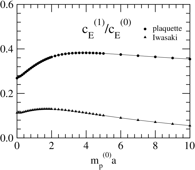
Figure 11: ${\it c}_{\it E}^{(1)}/{\it c}_{\it E}^{(0)}$ as a function of $m_{p}^{(0)}$. Solid lines denote the interpolation of ${\it c}_{\it E}^{(1)}/{\it c}_{\it E}^{(0)}$ with eq.(140)

In Fig. 11 we plot ${\it c}_{\it E}^{(1)}/{\it c}_{\it E}^{(0)}$ as a function of ${m_{p}^{(0)}}$ for the plaquette and the Iwasaki gauge actions. The fitting results of the interpolation

$$\frac{{\it c}_{\it E}^{(1)}}{{\it c}_{\it E}^{(0)}}=\left.\frac{{\it c}_{\it E}^{(1)}}{{\it c}_{\it E}^{(0)}}\right|_{{m_{p}^{(0)}}=0}+\frac{\sum_{i=1}^{5}a_{i}\{{m_{p}^{(0)}}\}^{i}}{1+\sum_{i=1}^{5}b_{i}\{{m_{p}^{(0)}}\}^{i}}$$ (140)

are also shown by the solid lines. We find relatively modest quark mass dependences similar to the ${\it c}_{\it B}$ case. The relative errors of this interpolation are less than a few % over the range $0<{m_{p}^{(0)}}\leq 10$. Table 6 summarizes the values of the parameters $a_{i}$ and $b_{i}$ ($i=1,\dots,5$) and ${\it c}_{\it E}^{(1)}/{\it c}_{\it E}^{(0)}$ at ${m_{p}^{(0)}}=0$ taken from Ref. csw_m0 .

VI Mean field improvement

In this section we rearrange the 1-loop results in the previous sections, using the mean-field improvement. We first replace the link variable $U_{n,\mu}$ by $u(U_{n,\mu}/u)=u{\tilde{U}}_{n,\mu}$, where $u$ is the average of the link variable $u=\langle U_{n,\mu}\rangle$ in some gauge fixing, or $u=P^{1/4}$ with $P$ is the average of the plaquette. In this paper, we adopt the latter definition:

$$u=1-g^{2}\frac{C_{F}}{2}T_{\rm MF}.$$ (141)

A detailed description on the derivation of $T_{\rm MF}$ is given in Sec. III of Ref. dwf_pt_rg .

This replacement leads to the following dispersion relation.

$$u\sinh({{\tilde{m}_{p}}^{(0)}}) = m_{0}+r_{t}(1-u\cosh({{\tilde{m}_{p}}^{(0)}}))+3r_{s}({{\tilde{m}_{p}}^{(0)}})(1-u)$$ (142)

$$= m+r_{t}u(1-\cosh({{\tilde{m}_{p}}^{(0)}}))+(1-u)3(r_{s}({{\tilde{m}_{p}}^{(0)}})-1)$$

where $m=m_{0}+r_{t}(1-u)+3(1-u)$ and ${{\tilde{m}_{p}}^{(0)}}$ is the tree level pole mass in the mean-field improvement. Using the relation

$$\sinh({m_{p}^{(0)}})+r_{t}\cosh({m_{p}^{(0)}}) = m+r_{t},$$ (143)

we have

$$(1+u-1)(\sinh({{\tilde{m}_{p}}^{(0)}})+r_{t}\cosh({{\tilde{m}_{p}}^{(0)}})) = \sinh({m_{p}^{(0)}})+r_{t}\cosh({m_{p}^{(0)}})$$ (144)

$$+ r_{t}(u-1)+(1-u)3(r_{s}({{\tilde{m}_{p}}^{(0)}})-1).$$

This leads to the relation:

$${m_{p}^{(0)}} = {{\tilde{m}_{p}}^{(0)}}+(u-1)\frac{\sinh({{\tilde{m}_{p}}^{(0)}})+r_{t}(\cosh({{\tilde{m}_{p}}^{(0)}})-1)+3(r_{s}({{\tilde{m}_{p}}^{(0)}})-1)}{\cosh({{\tilde{m}_{p}}^{(0)}})+r_{t}\sinh({{\tilde{m}_{p}}^{(0)}})}$$ (145)

$$\equiv {{{\tilde{m}_{p}}^{(0)}}}+g^{2}\Delta m_{p},$$

where

$$\Delta m_{p} = -\frac{C_{F}}{2}T_{MF}\frac{\sinh({{\tilde{m}_{p}}^{(0)}})+r_{t}(\cosh({{\tilde{m}_{p}}^{(0)}})-1)+3(r_{s}({{\tilde{m}_{p}}^{(0)}})-1)}{\cosh({{\tilde{m}_{p}}^{(0)}})+r_{t}\sinh({{\tilde{m}_{p}}^{(0)}})}.$$ (146)

Using this, the pole mass is rewritten as

$$m_{p} = {m_{p}^{(0)}}+g^{2}m_{p}^{(1)}={{{\tilde{m}_{p}}^{(0)}}}+g^{2}\tilde{m}_{p}^{(1)}$$ (147)

where $\tilde{m}_{p}^{(1)}=m_{p}^{(1)}+\Delta m_{p}$.

With the use of $\tilde{m}_{p}^{(1)}$ we apply the mean field improvement to $Z_{q}$, $\nu$, $r_{s}$, ${\it c}_{\it E}$ and ${\it c}_{\it B}$:

$$Z_{q,{\rm latt}} = Z_{q,{\rm latt}}^{(0)}({{\tilde{m}_{p}}^{(0)}})u\left(1+g^{2}\frac{Z_{q,{\rm latt}}^{(1)}}{Z_{q,{\rm latt}}^{(0)}}+g^{2}\frac{C_{F}}{2}T_{\rm MF}+\frac{g^{2}}{Z_{q,{\rm latt}}^{(0)}}\frac{\partial Z_{q,{\rm latt}}^{(0)}}{\partial{m_{p}^{(0)}}}{\Delta m_{p}}\right),$$ (148)

$$\nu = \nu^{(0)}({{\tilde{m}_{p}}^{(0)}})+g^{2}\nu^{(1)}({{\tilde{m}_{p}}^{(0)}})+g^{2}\frac{\partial\nu^{(0)}}{\partial{m_{p}^{(0)}}}{\Delta m_{p}},$$ (149)

$$r_{s} = r_{s}^{(0)}({{\tilde{m}_{p}}^{(0)}})+g^{2}r_{s}^{(1)}({{\tilde{m}_{p}}^{(0)}})+g^{2}\frac{\partial r_{s}^{(0)}}{\partial{m_{p}^{(0)}}}{\Delta m_{p}},$$ (150)

$${\it c}_{\it E} = {\it c}_{\it E}^{(0)}\frac{1}{u^{3}}\left(1+g^{2}\frac{{\it c}_{\it E}^{(1)}}{{\it c}_{\it E}^{(0)}}-g^{2}\frac{3}{2}C_{F}T_{\rm MF}+\frac{g^{2}}{{\it c}_{\it E}^{(0)}}\frac{\partial{\it c}_{\it E}^{(0)}}{\partial{m_{p}^{(0)}}}{\Delta m_{p}}\right),$$ (151)

$${\it c}_{\it B} = {\it c}_{\it B}^{(0)}\frac{1}{u^{3}}\left(1+g^{2}\frac{{\it c}_{\it B}^{(1)}}{{\it c}_{\it B}^{(0)}}-g^{2}\frac{3}{2}C_{F}T_{\rm MF}+\frac{g^{2}}{{\it c}_{\it B}^{(0)}}\frac{\partial{\it c}_{\it B}^{(0)}}{\partial{m_{p}^{(0)}}}{\Delta m_{p}}\right).$$ (152)

One then finally replaces $u=P^{1/4}$ with the one measured by Monte Carlo simulation.

The mean-field improved ${\overline{\rm MS}}$ coupling $g_{\overline{\rm MS}}^{2}(\mu)$ at the scale $\mu$ is obtained from the lattice bare coupling $g_{0}^{2}$ with the use of the following relation:

$$\displaystyle\frac{1}{g_{\overline{\rm MS}}^{2}(\mu)} = \displaystyle\frac{P}{g^{2}_{0}}+d_{g}+c_{p}+\displaystyle\frac{22}{16\pi^{2}}\log(\mu a)+N_{f}\left(d_{f}-\displaystyle\frac{4}{48\pi^{2}}\log(\mu a)\right).$$ (153)

For the improved gauge action one may use an alternative formulacppacs

$$\displaystyle\frac{1}{g_{\overline{\rm MS}}^{2}(\mu)} = \displaystyle\frac{c_{0}P+8c_{1}R1+16c_{2}R2+8c_{3}R3}{g^{2}_{0}}$$ (154)

$$+d_{g}+(c_{0}\cdot c_{p}+8c_{1}\cdot c_{R1}+16c_{2}\cdot c_{R2}+8c_{3}\cdot c_{R3})+\displaystyle\frac{22}{16\pi^{2}}\log(\mu a)$$

$$+N_{f}\left(d_{f}-\displaystyle\frac{4}{48\pi^{2}}\log(\mu a)\right),$$

where

$$P = \frac{1}{3}{\rm Tr}U_{pl}=1-c_{p}g_{0}^{2}+O(g_{0}^{4}),$$ (155)

$$R1 = \frac{1}{3}{\rm Tr}U_{rtg}=1-c_{R1}g_{0}^{2}+O(g_{0}^{4}),$$ (156)

$$R2 = \frac{1}{3}{\rm Tr}U_{chr}=1-c_{R2}g_{0}^{2}+O(g_{0}^{4}),$$ (157)

$$R3 = \frac{1}{3}{\rm Tr}U_{plg}=1-c_{R3}g_{0}^{2}+O(g_{0}^{4}),$$ (158)

and the measured values are employed for $P$, $R1$, $R2$ and $R3$. The values of $c_{p}$, $c_{R1}$, $c_{R2}$ and $c_{R3}$ for various gauge actions are listed in Table XVI of Ref. dwf_pt_rg .

VII Conclusion

In this paper we determine the $O(a)$ improvement coefficients, $\nu$, $r_{s}$, ${\it c}_{\it B}$ and ${\it c}_{\it E}$ in the relativistic heavy quark action up to the one-loop order for the various improved gauge actions. As byproducts we also calculate the quark wave function $Z_{q}$ and the pole mass $m_{p}$. While $\nu$, $r_{s}$, $Z_{q}$ and $m_{p}$ are determined from the quark propagator, we use the on-shell quark-quark scattering amplitude for ${\it c}_{\it B}$ and ${\it c}_{\it E}$. The $m_{Q}a$ dependences are examined by making the perturbative calculations done in the $m_{Q}a$ dependent way: As for the results of $\nu^{(1)}/\nu^{(0)}$, $r_{s}^{(1)}/r_{s}^{(0)}$, $Z_{q}^{(1)}/Z_{q}^{(0)}$ and $m_{p}^{(1)}$ we observe the strong $m_{Q}a$ dependence for $m_{Q}a\hbox to0.0pt{\lower 3.5pt\hbox{$\mathchar 0\relax\sim$}\hss}\raise 1.0pt\hbox{$<$}1$, while the dependence becomes much milder beyond $m_{Q}a\sim 1$. On the other hand, ${\it c}_{\it B}^{(1)}/{\it c}_{\it B}^{(0)}$ and ${\it c}_{\it E}^{(1)}/{\it c}_{\it E}^{(0)}$ show relatively mild $m_{Q}a$ dependences for $0<m_{Q}a\leq 10$. Employing the conventional perturbative method with the fictitious gluon mass to regularize the infrared divergence we show that the parameters $\nu$, $r_{s}$, ${\it c}_{\it B}$ and ${\it c}_{\it E}$ in the action are determined free from the infrared divergences. This is achieved if and only if the tree level values for $\nu$, $r_{s}$, ${\it c}_{\it B}$ and ${\it c}_{\it E}$ are properly adjusted as presented in Ref. akt . For later convenience we give a detailed description about how to apply the mean field improvement to our results. We are now trying a numerical test of this formulation with the mean field improved parameters employing the heavy-heavy and heavy-light meson systems.

Table 1: Values of parameters $a_{i}$ and $b_{i}$ ($i=1,2,3$) in the interpolation of ${m_{p}^{(0)}}$ with eq.(51) for the various gauge actions.

gauge action	$a_{1}$	$a_{2}$	$a_{3}$	$b_{1}$	$b_{2}$	$b_{3}$
plaquette	0.44498	1.1694	0.20262	5.1026	3.4713	1.3421
Iwasaki	0.33282	1.2533	0.24384	7.7008	7.4235	2.4353
Symanzik	0.39766	1.2161	0.22280	5.9914	4.6478	1.6915
Iwasaki’	0.33819	1.2549	0.23934	7.5388	7.1244	2.3482
Wilson	0.32642	1.2626	0.23357	7.9398	7.8574	2.5026
DBW2	0.25898	1.1989	0.24076	10.889	14.868	4.1077

Table 2: Values of parameters $a_{i}$ and $b_{i}$ ($i=1,\dots,4$) in the interpolation of $\Delta_{q}^{(1)}$ with eq.(60) for the various gauge actions. The values of $\Delta_{q}^{(1)}$ at ${m_{p}^{(0)}}=0$ are taken from Ref. gmass except for the DBW2 gauge action. gauge action $\Delta_{q}^{(1)}({m_{p}^{(0)}}=0)$ $a_{1}$ $a_{2}$ $a_{3}$ $a_{4}$ $b_{1}$ $b_{2}$ $b_{3}$ $b_{4}$ plaquette $-$0.07773 0.18777 3.1560 $-$0.15124 0.090311 15.929 11.134 0.83734 0.44445 Iwasaki $-$0.01478 0.088032 4.5405 $-$0.59509 0.12110 48.391 27.665 $-$1.7715 0.83723 Symanzik $-$0.05044 0.13224 4.0242 $-$0.51558 0.20496 25.697 17.632 $-$0.67533 1.3005 Iwasaki’ $-$0.01739 0.093314 2.8033 $-$0.37819 0.078356 28.654 16.445 $-$1.1042 0.53359 Wilson $-$0.01068 0.082214 3.4543 $-$0.40922 0.085302 39.349 21.267 $-$1.0475 0.56718 DBW2 $+$0.02029 0.036401 0.33748 0.19697 0.027077 9.0916 6.0990 3.1026 0.11858

Table 3: Values of parameters $a_{i}$ and $b_{i}$ ($i=1,\dots,5$) in the interpolation of $\nu^{(1)}$ with eq.(63) for the various gauge actions. gauge action $a_{1}$ $a_{2}$ $a_{3}$ $a_{4}$ $a_{5}$ $b_{1}$ $b_{2}$ $b_{3}$ $b_{4}$ $b_{5}$ plaquette 0.0013787 0.23077 2.3586 0.41097 0.21571 21.776 23.401 16.822 1.0718 2.0084 Iwasaki 0.010681 0.10966 1.4455 0.29523 0.14143 17.745 29.424 21.954 1.3323 2.7265 Symanzik 0.0063804 0.18587 1.9939 0.37153 0.18560 20.428 26.116 18.407 1.2431 2.2404 Iwasaki’ 0.010248 0.11663 1.4875 0.30469 0.14531 17.882 28.950 21.577 1.3199 2.6761 Wilson 0.010284 0.10466 1.3679 0.29382 0.13690 16.951 28.693 22.473 1.2577 2.7941 DBW2 0.011730 0.021615 0.77692 0.18009 0.085451 13.817 30.339 31.211 0.83789 3.8899

Table 4: Values of parameters $a_{i}$ and $b_{i}$ ($i=1,\dots,5$) in the interpolation of $r_{s}^{(1)}$ with eq.(67) for the various gauge actions. gauge action $a_{1}$ $a_{2}$ $a_{3}$ $a_{4}$ $a_{5}$ $b_{1}$ $b_{2}$ $b_{3}$ $b_{4}$ $b_{5}$ plaquette 0.048659 0.23362 1.6049 0.15709 0.068748 6.9070 18.195 11.853 0.74864 0.92944 Iwasaki 0.0015650 $-$0.14504 1.3871 0.012363 0.044884 12.493 27.761 31.031 $-$2.4872 2.0163 Symanzik 0.024680 0.14420 0.92264 0.11171 0.044813 6.8434 12.778 12.079 0.010953 0.97640 Iwasaki’ 0.012139 $-$0.18772 2.3352 0.037267 0.080842 20.355 42.341 48.503 $-$3.5202 3.1917 Wilson 0.015805 $-$0.14494 1.9526 $-$0.034214 0.066725 17.479 36.192 41.823 $-$3.7429 2.5913 DBW2 $-$0.038636 $-$0.21232 0.44240 $-$0.11604 0.015381 5.3026 20.770 22.879 $-$9.2470 1.6088

Table 5: Values of parameters $a_{i}$ and $b_{i}$ ($i=1,\dots,5$) in the interpolation of ${\it c}_{\it B}^{(1)}$ with eq.(117) for the various gauge actions. The values of ${\it c}_{\it B}^{(1)}/{\it c}_{\it B}^{(0)}$ at ${m_{p}^{(0)}}=0$ are taken from Ref. csw_m0 . gauge action ${\it c}_{\it B}^{(1)}/{\it c}_{\it B}^{(0)}({m_{p}^{(0)}}=0)$ $a_{1}$ $a_{2}$ $a_{3}$ $a_{4}$ $a_{5}$ $b_{1}$ $b_{2}$ $b_{3}$ $b_{4}$ $b_{5}$ plaquette 0.26858825 0.11031 $-$0.45775 1.4585 3.5629 0.19832 $-$1.2454 6.9947 72.053 7.4057 6.4400 Iwasaki 0.11300591 0.031328 $-$0.25330 $-$0.97944 4.9518 $-$0.70873 11.329 $-$16.089 275.53 27.127 13.769 Symanzik 0.19624449 0.070876 $-$0.35318 0.75783 2.6525 $-$0.034442 $-$2.6878 6.1987 70.755 8.3789 5.2277 Iwasaki’ 0.12036501 0.025289 $-$0.18878 0.14872 1.3433 $-$0.17271 $-$0.73798 9.9278 71.365 8.0592 3.6373 Wilson 0.10983411 0.021005 $-$0.19478 0.16783 0.93978 $-$0.15323 $-$0.74965 11.415 64.418 7.0567 2.8708 DBW2 0.04243181 8.7741 $-$14.110 $-$19.180 1.0685 $-$5.2296 $-$516.57 1177.1 76.371 472.69 37.314

Table 6: Values of parameters $a_{i}$ and $b_{i}$ ($i=1,\dots,5$) in the interpolation of ${\it c}_{\it E}^{(1)}$ with eq.(140) for the various gauge actions. The values of ${\it c}_{\it E}^{(1)}/{\it c}_{\it E}^{(0)}$ at ${m_{p}^{(0)}}=0$ are taken from Ref. csw_m0 . gauge action ${\it c}_{\it E}^{(1)}/{\it c}_{\it E}^{(0)}({m_{p}^{(0)}}=0)$ $a_{1}$ $a_{2}$ $a_{3}$ $a_{4}$ $a_{5}$ $b_{1}$ $b_{2}$ $b_{3}$ $b_{4}$ $b_{5}$ plaquette 0.26858825 0.061511 $-$0.52275 1.5301 0.087055 $-$0.009142 $-$8.4208 27.507 $-$2.5724 3.1868 $-$0.15206 Iwasaki 0.11300591 0.014754 $-$0.16103 0.47732 $-$0.093278 $-$0.0044554 $-$5.8133 21.985 $-$1.4805 1.7759 $-$0.025592 Symanzik 0.19624449 0.046299 $-$0.38345 1.0557 $-$0.013178 $-$0.0040176 $-$7.9568 23.808 $-$1.5669 2.4568 $-$0.058986 Iwasaki’ 0.12036501 $-$1.0186 10.033 $-$0.22227 $-$0.57195 0.048774 533.27 $-$178.18 147.82 $-$22.688 0.92777 Wilson 0.10983411 21.659 $-$158.46 271.84 $-$50.696 1.1180 $-$3836.5 8792.4 $-$268.31 644.04 $-$28.188 DBW2 0.04243181 $-$0.084945 $-$0.49122 $-$0.61820 0.13749 $-$0.069162 $-$1.2883 45.147 $-$10.501 2.9737 0.14473

Figure 1: Momentum assignment for the quark-gluon vertices.

Figure 2: Momentum assignment for the three-gluon vertex.

Figure 3: One-loop diagrams for the quark self-energy.

Figure 8: Tree level diagrams for the quark-quark scattering.

Figure 9: Quark-gluon vertex at the one-loop level.