Phase structure of lattice QCD for general number of flavors

Abstract

We investigate the phase structure of lattice QCD for the general number of flavors in the parameter space of gauge coupling constant and quark mass, employing the one-plaquette gauge action and the standard Wilson quark action. Performing a series of simulations for the number of flavors $N_{F}=6$–360 with degenerate-mass quarks, we find that when $N_{F}\geq 7$ there is a line of a bulk first order phase transition between the confined phase and a deconfined phase at a finite current quark mass in the strong coupling region and the intermediate coupling region. The massless quark line exists only in the deconfined phase.

Based on these numerical results in the strong coupling limit and in the intermediate coupling region, we propose the following phase structure, depending on the number of flavors whose masses are less than $\Lambda_{d}$ which is the physical scale characterizing the phase transition in the weak coupling region: When $N_{F}\geq 17$, there is only a trivial IR fixed point and therefore the theory in the continuum limit is free. On the other hand, when $16\geq N_{F}\geq 7$, there is a non-trivial IR fixed point and therefore the theory is non-trivial with anomalous dimensions, however, without quark confinement. Theories which satisfy both quark confinement and spontaneous chiral symmetry breaking in the continuum limit exist only for $N_{F}\leq 6$.

I Introduction

The fundamental properties of QCD are quark confinement, asymptotic freedom and spontaneous breakdown of chiral symmetry. Among them, the asymptotic freedom is lost when the number of flavors exceeds $16\frac{1}{2}$. Thus the question which naturally arises is what is the constraint on the number of flavors for quark confinement and/or the spontaneous breakdown of chiral symmetry.

As asymptotic freedom is the nature at short distances, one can apply the perturbation theory to investigate the critical number for it. However, because quark confinement and spontaneous chiral symmetry breaking are due to non-perturbative effects, one has to apply a non-perturbative method throughout the investigation of the critical numbers for them. We employ lattice QCD for the investigation in this work, since lattice QCD is the only known theory of QCD which is constructed non-perturbatively.

Lattice QCD is a theory with fundamental parameters, the gauge coupling constant $g$ and quark masses $m_{q}$, defined on a lattice with lattice spacing $a$. The inverse of the lattice spacing $a^{-1}$ plays a role of an UV cutoff. In order to investigate properties of the theory in the continuum limit, one has to first clarify the phase structure of lattice QCD at zero temperature for general number of flavors, and then identify an UV fixed point and/or an IR fixed point of an RG (Renormalization Group) transformation. When the existence of such fixed points is established, one is able to conclude what kind of theory exists in the continuum limit.

In our previous work previo , it was shown that, even in the strong coupling limit, when the number of flavors $N_{F}$ is greater than or equal to seven, quarks are deconfined and chiral symmetry is restored at zero temperature, if the quark mass is lighter than a critical value which is of order $a^{-1}$.

In this work we extend the region of the gauge coupling constant to weaker ones, and investigate the phase diagram for general number of flavors $N_{F}$ at zero temperature. We mainly consider the case where $N_{F}$ quark masses are degenerate. However, we also discuss the non-degenerate case.

We employ the simplest form of the action in this work, that is, the Wilson quark action and the standard one-plaquette gauge action. At finite lattice spacings, the Wilson quark action is not chirally symmetric even at vanishing bare quark mass due to the Wilson term which is added to a naive discretized Dirac action in order to lift the doublers. Because of the fact that the action does not hold chiral symmetry, the phase diagram becomes complicated in general.

As the phase diagram turns out to be complicated on the lattice, we first give a brief summary in terms of the $\beta$ function in Sec. II. Further, the phase diagram for general number of flavors when the theory would be chirally symmetric is conjectured in Sec. III. This conjecture is based on our proposal for the phase diagram for the lattice action we employ, and is given because it may help the reader to understand the whole structure of the phase diagram. After showing the brief summary in this way, the action we employ is given with some basic notations in Sec. IV. Here some important facts related to chiral property of the quark are also discussed. Then the main part of the paper, our proposal for the phase structure for the general number of flavors in the case of the Wilson quark action, is summarized in Sec. V, before giving the detailed numerical results which lead to our proposal. We also comment on previous results obtained with the staggered quark action. After giving numerical parameters for our simulations in Sec. VI, numerical results in the strong coupling limit and at finite coupling constants are given in Secs. VII and VIII, respectively. All the investigations up to this point are limited to the degenerate quark mass case. In Sec. IX, we extend the study to the non-degenerate case to discuss implication for physics. We give a summary in Sec. X. In an Appendix, we study the case of $N_{c}=2$ in the strong coupling limit. Preliminary results of our study have been presented in Refs. lat94 ; report97 .

II Phase structure in terms of beta function

The perturbative beta function of QCD with $N_{F}$ flavors of massless quarks is universal up to two-loop order:

$$\tilde{\beta}(g)=-b_{0}g^{3}-b_{1}g^{5}+\cdots,$$ (1)

where

$$b_{0}=\frac{1}{16\pi^{2}}\left(11-\frac{2}{3}N_{F}\right)$$ (2)

and

$$b_{1}=\frac{1}{(16\pi^{2})^{2}}\left(102-\frac{38}{3}N_{F}\right).$$ (3)

The coefficient $b_{0}$ changes its sign at $N_{F}=16\frac{1}{2}$. Hence, for $N_{F}\geq 17$, asymptotic freedom is lost and the point $g=0$ is an IR fixed point. The theory governed by this IR fixed point is a free theory and the quark is not confined. The second coefficient $b_{1}$ changes its sign at $N_{F}\approx 8.05$. This implies, if one would take the two-loop form of the beta-function, that an IR fixed point appears at finite coupling constant for $9\leq N_{F}\leq 16$. Of course we cannot trust the two-loop form at finite coupling constants. However, since the IR fixed point from the two-loop beta function locates in a weak coupling region for $N_{F}\sim 16$, it is plausible that the beta function has a non-trivial IR fixed point for $N^{\prime}\leq N_{F}\leq 16$ with some $N^{\prime}\leq 16$. When such an IR fixed point exists, the coupling constant cannot become arbitrarily large in the IR region. This implies that quarks are not confined. The long distance behavior of the theory is governed by the non-trivial IR fixed point: It is a theory with an anomalous dimension.

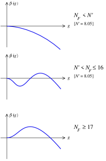
a) b)

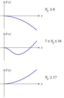
Figure 1: Renormalization group beta function. (a) Conjecture by Banks and Zaks Banks1 assuming confinement in the strong coupling limit for all $N_{F}$. (b) Our conjecture deduced from the results of lattice simulations.

A pioneering study on the $N_{F}$ dependence of the QCD vacuum was made by Banks and Zaks in 1982 Banks1 . Based on the result of the quark confinement in a pure gauge theory Kogut79 , they assumed that the quark is confined and that the beta function is negative in the strong coupling limit for all $N_{F}$. Using the perturbative results mentioned above, they conjectured Fig. 1(a) as the simplest $N_{F}$ dependence of the beta function, and studied the phase structure of QCD based on this $N_{F}$ dependence of the beta function. Because of an additional non-trivial UV fixed point for $N_{F}>N^{\prime}$, their conjecture for the phase structure is complicated.

In the argument of Banks and Zaks, the assumption of confinement and negative beta function in the strong coupling limit plays an essential role. However, there exist no proofs of confinement in QCD for general $N_{F}$ even in the strong coupling limit. A non-perturbative investigation on the lattice is required. Therefore, in our previous work previo , we performed numerical simulations of QCD in the strong coupling limit for various $N_{F}$, using the Wilson fermion formalism for lattice quarks. We found that, when $N_{F}\geq 7$, quarks are deconfined and chiral symmetry is restored at zero temperature even in the strong coupling limit, when the quark mass is lighter than a critical value.

In some previous literatures, quark confinement in the strong coupling limit has been assumed explicitly or implicitly. However, the arguments for the confinement in the strong coupling limit are based on either the large $N_{c}$ limit SCENc , a meanfield approximation ($1/d$ expansion) SCEmf ; SCEmfMq , or a heavy quark mass expansion SCEmfMq ; wilson77 . Because we are interested in the theory with dynamical quarks with $N_{c}$ kept 3, and effects of dynamical quarks become significant only when they are light, the results of these approximations cannot be applied. Actually, our numerical result at $g=\infty$ explicitly shows violation of quark confinement at small quark masses when $N_{F}\geq 7$.

Here we extend the study to weaker couplings. Based on the numerical results obtained on the lattice (see the following sections for details) combined with the results of the perturbation theory, we conjecture Fig. 1(b) for the $N_{F}$ dependence of the beta function: When $N_{F}\leq 6$, the beta function is negative for all values of $g$. Quarks are confined and the chiral symmetry is spontaneously broken at zero temperature. (Corresponding critical $N_{F}$ is 2 for the case $N_{c}=2$ lat94 . See the discussion in the Appendix.) On the other hand, when $N_{F}$ is equal or larger than 17, we conjecture that the beta function is positive for all $g$, in contrast to the conjecture by Banks and Zaks shown in Fig. 1(a). The theory is trivial in this case. When $N_{F}$ is between 7 and 16, the beta function changes sign from negative to positive with increasing $g$. Therefore, the theory has a non-trivial IR fixed point.

Here we note that there are several related works which do not use lattice formulation Oehme ; Nishijima ; Appelquist ; sigma . These works gave interesting results for the quark confinement condition. However, the critical number for the confinement is at most suggestive, because we need fully non-perturbative method to investigate the problem. That is, the theory should be constructed from the beginning non-perturbatively. In this regards, lattice QCD is the only known theory constructed non-perturbatively.

III Conjecture for the Phase diagram in Chirally Symmetric Case

In this section, we present our conjecture for the phase diagram of QCD, for the case when the theory is chiral symmetric. The conjecture is based on the phase diagram we propose for the case of the Wilson fermion action, where the chiral symmetry is violated. The reason why we make this kind of conjecture is that it may help the reader to understand the phase diagram of the Wilson fermion action which is more complicated. The phase diagrams we conjecture in the $g-m_{0}$ plane are presented in Fig. 2.

a)

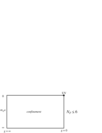
b)

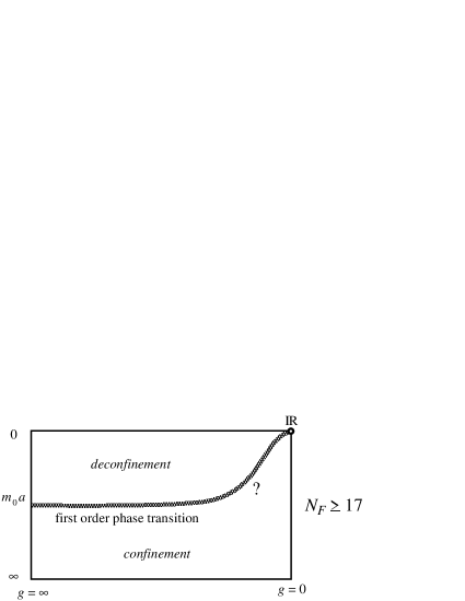
c)

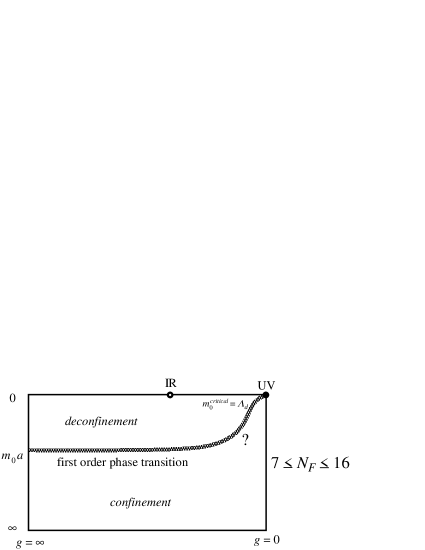
Figure 2: Phase diagram for a chirally symmetric case. (a) $N_{F}\leq 6$, (b) $N_{F}\geq 17$, (c) $7\leq N_{F}\leq 16$.

III.1 $N_{F}\leq 6$

The phase diagram is simple. At zero temperature all the region is in the confined phase. See Fig. 2(a).

III.2 $N_{F}\geq 17$

At zero temperature, there is a first-order phase transition which separates a deconfined phase from the confined phase. The transition occurs at $m_{0}^{critical}$ which is of the same order of magnitude as the inverse of a typical correlation length $\xi$ of gluon dynamics, such as the plaquette-plaquette correlation length.

In the confined phase, the nature of the system is essentially same as that for $N_{F}\leq 6$: When $m_{0}\gg\xi^{-1}$, dynamical effects by quark loops can be neglected. In this case, the system is equivalent to the quenched QCD. That is, for $m_{0}\gg\xi^{-1}$ the phase is the confined phase. When dynamical effects of quark loops change the phase from that in the quenched case, there will be a phase transition in general, and this kind of the transition occurs at $m_{0}\sim\xi^{-1}$.

When the gauge coupling decreases towards zero, the dimension-less correlation length $\xi/a$ increases and diverges at zero coupling constant in the confined phase. Therefore, along the phase transition line, the dimension-less critical quark mass should behave as $m_{0}^{critical}a=\Lambda_{d}a$. Here $a$ vanishes towards $g=0$, and $\Lambda_{d}\sim\xi^{-1}$ is the physical scale which characterizes the phase transition in the weak coupling region.

The “?” mark in the weak coupling region means that we have performed numerical simulation for only the strong and intermediate coupling regions because of technical reason. In this sense, our proposal for the strong and intermediate coupling regions is based on our numerical results, while our conjecture in the weak region is based on the assumption that the transition occurs at $m_{0}^{critical}\sim\xi^{-1}$.

In the upper region above the phase transition line quarks are not confined. There is only an IR fixed point at $g=0$. That is, the theory in the continuum limit is free.

We would like to make a comment that there is an alternative possibility that the transition occurs at $m_{0}^{critical}\sim a^{-1}$, where $a^{-1}$ is the inverse of the lattice spacing. In the strong and intermediate coupling regions $\xi^{-1}$ is of order $a^{-1}$. Therefore, there is no essential difference between the two possibilities whether $m_{0}^{critical}\sim a^{-1}$ or $m_{0}^{critical}\sim\xi^{-1}$.

In the usual argument of the decoupling theorem for QCD, the effect of the particle whose mass is much heavier than the QCD scale parameter $\Lambda_{QCD}$ can be absorbed by renormalization of physical quantities. Based on a similar consideration, one may argue that the particles whose masses are much heavier than $\Lambda_{QCD}$ are irrelevant for quark confinement. This is the reason why we assume that the transition occurs at $m_{0}^{critical}\sim\xi^{-1}$. However, whether a theory exists in a sense of constructive field theory is a different problem. Therefore, we think that it is not possible to disregard the alternative possibility of $m_{0}^{critical}\sim a^{-1}$ only from a theoretical argument.

Nonetheless we think that the assumption that the transition occurs at $m_{0}^{critical}\sim\xi^{-1}$ is more plausible than the assumption $m_{0}^{critical}\sim a^{-1}$. In the following we assume that the phase transition occurs at $m_{0}^{critical}\sim\xi^{-1}$. This is our conjecture.

However, we also refer to the alternative possibility of $m_{0}^{critical}\sim a^{-1}$ when it is appropriate to refer to. In this alternative case, the transition point at $g=0$ is off the massless point and therefore all finite massive quarks belong to the deconfined phase.

It will be possible to see in future which of $m_{0}^{critical}\sim a^{-1}$ or $m_{0}^{critical}\sim\xi^{-1}$ is realized by numerical simulations.

III.3 $7\leq N_{F}\leq 16$

The phase diagram at zero temperature shown in Fig. 2(c) is similar to that in the case of $N_{F}\geq 17$. The phase transition line locates around $m_{0}\sim\xi^{-1}$, due to the same reason as in the case of $N_{F}\geq 17$.

However, the flow of RG transformation is different. The $g=0$ point in this case is an UV fixed point, contrary to the case $N_{F}\geq 17$. On the other hand, quarks are deconfined in the upper region above the phase transition line as in the case of $N_{F}\geq 17$. Therefore there should be an IR fixed point at finite coupling constant. Otherwise gauge coupling would become arbitrary large at large distance, and quarks would be confined in the strong coupling limit contrary to the result of the numerical simulation.

IV Fundamentals of Lattice QCD and the Action

Lattice QCD is defined on a hypercubic lattice in 4-dimensional euclidean space with lattice spacing $a$. A site is denoted by a vector $n=(n_{1},n_{2},n_{3},n_{4})$, where $n_{i}$’s are integers. A link with end points at the sites $n$ and $n+\hat{\mu}$ is specified by a pair $(n,\mu)$, where $\hat{\mu}$ denotes a unit vector in the $\mu$ direction.

IV.1 Action

The gauge variable $U_{n,\mu}$ which is an element of SU(3) gauge group is defined on the link $(n,\mu)$. The action for gluons which we adopt is given by

$$S_{gauge}=\frac{1}{g^{2}}\sum_{n,\mu\neq\nu}{\rm Tr}(U_{n,\mu}U_{n+\hat{\mu},\nu}U_{n+\hat{\mu}+\hat{\nu},\mu}^{{\dagger}}U_{n+\hat{\nu},\nu}^{{\dagger}}),$$ (4)

where g is the gauge coupling constant. This action is called the standard one-plaquette gauge action. We usually use, instead of the bare gauge coupling constant $g$, $\beta$ defined by

$$\beta=\frac{6}{g^{2}}.$$ (5)

The quark variable is a Grassmann number defined on each site. It is well-known that a naive discretization of the Dirac action

$$S_{fermion} = \frac{a^{3}}{2}\sum_{n,\mu}(\bar{q}_{n}\gamma_{\mu}q_{n+\hat{\mu}}-\bar{q}_{n+\hat{\mu}}\gamma_{\mu}q_{n})$$ (6)

$$+m_{0}a^{4}\sum_{n}\bar{q}_{n}q_{n},$$

with $m_{0}$ being the bare fermion mass, leads to $16$ poles instead of one pole. This problem is called the species doubling. To avoid this problem K. Wilson proposed to add a dimension 5 operator called the Wilson term

$$-a^{3}\sum_{n,\mu}(\bar{q}_{n}q_{n+\hat{\mu}}-2\bar{q}_{n}q_{n}+\bar{q}_{n+\hat{\mu}}q_{n}),$$ (7)

to the naive discretized action. Rescaling the fermion field by $q=\sqrt{2K}\psi$ and making the action gauge invariant, we obtain the Wilson fermion action

$$S_{Wilson} = a^{3}\sum_{n}[\bar{\psi}_{n}\psi_{n}-K\{\bar{\psi}_{n}(1-\gamma_{\mu})U_{n,\mu}\psi_{n+\hat{\mu}}$$ (8)

$$+\bar{\psi}_{n+\hat{\mu}}(1+\gamma_{\mu})U_{n,\mu}^{{\dagger}}\psi_{n}\}].$$

where

$$K=\frac{1}{2(m_{0}a+4)},$$ (9)

which is called the hopping parameter.

The full action $S$ is given by the sum of the gauge part $S_{gauge}$ and the fermion part $S_{Wilson}$,

$$S=S_{gauge}+\sum_{f=1}^{N_{F}}S_{Wilson},$$ (10)

where $f$ is for flavors.

The expectation value of an operator ${\cal O}(U,\psi,\bar{\psi})$ is given by

$$\langle{\cal O}\rangle=\frac{1}{Z}\int\prod_{n,\mu}{\rm d}U_{n,\mu}\prod_{n,f}{\rm d}\psi_{n}^{(f)}{\rm d}\bar{\psi}_{n}^{(f)}{\cal O}(U,\psi,\bar{\psi}){\rm exp}(S),$$ (11)

where $Z$ is the partition function

$$Z=\int\prod_{n,\mu}{\rm d}U_{n,\mu}\prod_{n,f}{\rm d}\psi_{n}^{(f)}{\rm d}\bar{\psi}_{n}^{(f)}{\rm exp}(S),$$ (12)

with ${\rm d}U_{n,\mu}$ being the Haar measure of SU(3).

IV.2 Fundamental parameters

In the case of degenerate $N_{F}$ flavors, lattice QCD contains two parameters: the gauge coupling constant $\beta=6/g^{2}$ and the bare quark mass or the hopping parameter $K=1/(m_{0}a+4)$. In the non-degenerate case, we have, in general, $N_{F}$ independent bare masses (hopping parameters).

In this work we consider mainly the case where $N_{F}$ quark masses are degenerate, because it is simpler. However, the conjecture can be extended to non-degenerate cases. We will discuss this point in Sec. IX.

IV.3 Continuum limit

As mentioned in the Introduction, in order to see what kind of theory in the continuum limit exists, one has to investigate the phase structure and identify UV fixed points and IR fixed points.

When the $g=0$ point is an UV fixed point, the theory governed by this fixed point is an asymptotically free theory. On the other hand, when the $g=0$ point is an IR fixed point, the theory governed by this fixed point is a free theory. When there is a IR fixed point at finite coupling constant $g$, the theory is a non-trivial theory with the long distance behavior determined by the IR fixed point.

IV.4 Finite temperatures

At finite temperatures the linear extension in the time direction $N_{t}$ is much smaller than those in the spatial directions ($N_{x},N_{y},N_{z}$). The temperature $T$ is given by $1/N_{t}a.$ For gluons the periodic boundary condition is imposed, while for quarks an anti-periodic boundary condition is imposed in the time direction.

Although we are interested in the phase structure of lattice QCD at zero temperature, we investigate phase transitions on lattices at finite temperatures. Increasing the value of $N_{t}$, we carefully examine the $N_{t}$ dependence of the phase transition. If the transition is $N_{t}$ independent for sufficiently large $N_{t}$, then the transition is a bulk transition (phase transition at zero temperature).

IV.5 Quark mass and chiral symmetry

In the Wilson quark formalism, the flavor symmetry as well as C, P and T symmetries are exactly satisfied on a lattice with a finite lattice spacing. However, chiral symmetry is explicitly broken by the Wilson term even for the vanishing bare quark mass $m_{0}=0$ at finite lattice spacings. The lack of chiral symmetry causes much conceptual and technical difficulties in numerical simulations and physics interpretation of data. (See for more details Ref. Stand26 and references cited there.)

The chiral property of the Wilson fermion action was first systematically investigated through Ward-Takahashi identities by Bochicchio et al. Bo . We also independently proposed ItohNP to define the current quark mass by

$$2m_{q}\langle\,0\,|\,P\,|\,\pi\,\rangle=-m_{\pi}\langle\,0\,|\,A_{4}\,|\,\pi\,\rangle,$$ (13)

where $P$ is the pseudoscalar density and $A_{4}$ the fourth component of the local axial vector current. We use this definition of the current quark mass as the quark mass in this work. In general we need multiplicative normalization factors for the pseudoscalar density and the axial current. In this study, we absorb these renormalization factors into the definition of the quark mass, because this definition is sufficient for later use. We note that the quark mass thus defined has an additive renormalization constant to the bare quark mass, because the Wilson quark action does not hold chiral symmetry.

With this definition of quark mass, when the quark is confined and the chiral symmetry is spontaneously broken, the pion mass vanishes in the chiral limit where the quark mass vanishes at zero temperature.

However, in the deconfined phase at finite temperatures the pion mass does not vanish in the chiral limit. It is almost equal to twice the lowest Matsubara frequency $\pi/N_{t}$. This implies that the pion state is approximately a free two-quark state. The pion mass is nearly equal to the scalar meson mass, and the rho meson mass to the axial vector meson mass; they are all nearly equal to the twice the lowest Matsubara frequency $\pi/N_{t}$. Thus the chiral symmetry is also manifest within corrections due to finite lattice spacing.

In a previous study Wqmass we found that, given the gauge coupling constant and bare quark masses, the value of the quark mass does not depend on whether the system is in the high or the low temperature phase when the gauge coupling is not so strong: $\beta\geq 5.5$ for $N_{F}=2$. However, this property is not guaranteed for smaller $\beta$. In general, the quark mass in the deconfined phase differs from that in the confined phase in the strong coupling region.

IV.6 Quark mass at $g=0$

As mentioned earlier, the Wilson term (7) lifts the doublers and retains only one pole around $m_{0}=0$ in the free case. On the other hand, there are other poles at different values of the bare masses. They are remnants of the doublers.

a)

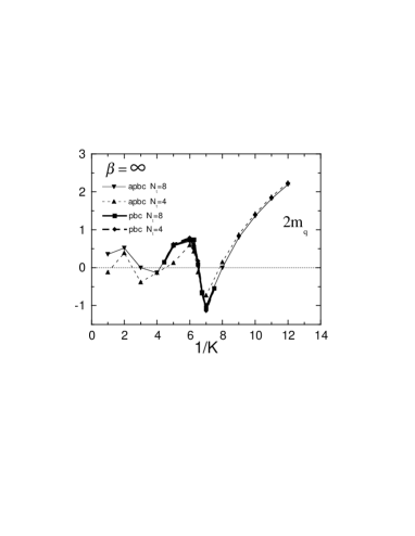
b)

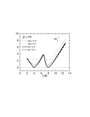
Figure 3: (a) $m_{q}$ at $\beta=\infty$. (b) $m_{\pi}$ at $\beta=\infty$. Results with an anti-periodic boundary condition (apbc) in the $t$-direction and those with the periodic boundary condition (pbc) are compared on $N_{t}=8$ and 4 lattices.

In Fig. 3(a) the quark mass defined by (13) is plotted versus the bare quark mass for the case of free Wilson quark. At $m_{0}\geq 0$ ($1/K\geq 8$) the quark mass behaves as expected: it monotonously increases with $m_{0}$. On the other hand, at $m_{0}\leq 0$ ($1/K\leq 8$) the behavior of the quark mass is complicated: it does not monotonously decrease with decreasing $m_{0}$, but increases after some decrease and becomes zero at a finite negative value of $m_{0}$. Usually, the region of negative bare quark mass is irrelevant for numerical calculations of physical quantities. However, this region is also important for understanding the phase diagram.

We also plot in Fig. 3(b) the mass of the pion which is composed of two free quarks with periodic boundary condition for the time direction and with anti-periodic boundary condition. These results will be referred to later.

a)

b)

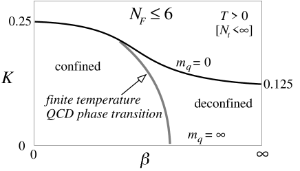
Figure 4: The phase structure for $N_{F}\leq 6$; (a) at zero temperature, and (b) at finite temperatures. The chiral limit (massless quark limit) is shown by thick curves labeled by “$m_{q}=0$”, and the finite temperature QCD transition at a fixed finite $N_{t}$ is shown by a shaded curve.

V Phase diagram

Here we propose, based on our numerical results which will be shown later and the perturbation theory, the phase diagram in the $(\beta,K)$ plane for the Wilson quark action coupled with the one-plaquette gauge action.

V.1 $N_{F}\leq 6$

For $N_{F}\leq 6$, the chiral line $K_{c}(\beta)$ where the current quark $m_{q}$ vanishes, exists in the confined phase(See Fig. 4(a)). The value of $K_{c}(\beta)$ at $\beta=\infty$ is 1/8, which corresponds to the vanishing bare quark mass $m_{0}=0$. As $\beta$ is decreased, the value of $K_{c}$ increases up to 1/4 at $\beta=0$. If the action would be chiral symmetric, the chiral line should be a constant, 1/8, as in Sec. III. The line $K=0$ corresponds to the case of infinitely heavy quarks. Quarks are confined for any value of the current quark mass for all values of $\beta$ at zero temperature ($N_{t}=\infty$).

On a lattice with a fixed finite $N_{t}$, we have the finite temperature deconfining transition at finite $\beta$, because the temperature $T=1/N_{t}\,a$ becomes larger as $\beta$ increases in asymptotically free theories. At $K=0$ ($m_{q}=\infty$), the first order finite temperature phase transition of pure SU(3) gauge theory locates at $\beta_{c}=5.69254(24)$ and 5.89405(51) for $N_{t}=4$ and 6 QCDPAX and at $\beta_{c}\simeq 6.0625$ for $N_{t}=8$ Boyd96 . This finite temperature transition turns into a crossover transition at intermediate values of $K$, and becomes stronger again towards the chiral limit $K_{c}$. As $K$ is increased, the finite temperature transition line crosses the $K_{c}$ line at finite $\beta$ Stand26 . We note that, for understanding the whole phase structure which includes the region above the $K_{c}$ line (negative values of the bare quark mass), the existence of the Aoki phase is important Aoki . A schematic diagram of the phase structure for this case is shown in Fig. 4(b). For simplicity, we omit the phase structure above the $K_{c}$ line. It is known that the system is not singular on the $K_{c}$ line in the high-temperature phase (to the right of the finite temperature transition line) Stand26 . The location of the finite temperature transition line moves toward larger $\beta$ as $N_{t}$ is increased. In the limit $N_{t}=\infty$, the finite temperature transition line will shift to $\beta=\infty$ so that only the confined phase is realized at $T=0$.

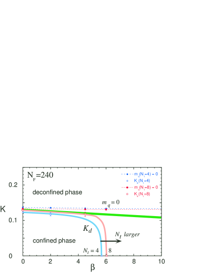
Figure 5: Phase diagram for $N_{F}=240$. Dark shaded (green) lines represent our conjecture for the bulk transition line in the limit $N_{t}=\infty$. Points connected by dashed lines are the measured points where quarks are massless. Light shaded lines are for the finite temperature transition at $N_{t}=4$ and 8.

V.2 When $N_{F}$ is very large

We present the result for the case of $N_{F}=240$ in Fig. 5. The reason why we investigate the case where the number of flavor is so large as 240 is the following: We have first investigated the case of $N_{F}=18$ as a generic case for $N_{N}\geq 17$. However it has turned out that the phase diagram looks complicated when $N_{F}=18$. So, to understand the phase structure for $N_{F}\geq 17$, we have increased the number of flavors like 18, 60, 120, 180, 240, and 300, and systematically viewed the results of the quark mass and the pion mass for all these numbers of flavors. Then we have found that when the number of flavors is very large as 240, the phase diagram is simple as the chirally symmetric case discussed in Sec. III. Therefore we first show the result for the case of $N_{F}=240$.

At finite $N_{t}$ where numerical simulations have been performed, the finite temperature transition occurs as shown in Fig. 5. As $N_{t}$ increases, the transition line moves towards larger value of $\beta$. The envelop of those finite temperature transition lines is the zero temperature phase transition line, shown by the dark shaded curve in the figure. Note that, at finite $N_{t}$, the system is not singular on the part of the dark shaded line in the right hand side of the finite temperature transition line (i.e., in the high temperature phase).

The salient fact is that, at zero temperature, the massless line exists only in the deconfined phase and passes through from $\beta=0$ down to $\beta=\infty$, i.e., it is quite similar to the chirally symmetric case of $N_{F}\geq 17$ shown in Fig. 2(b). Thus the IR fixed point at $g=0$ governs the long distance behavior of the theory and therefore the theory is a free theory.

a)

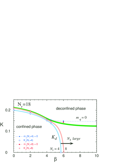
b)

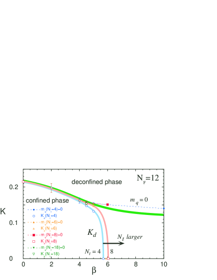
Figure 6: The same as Fig. 5, but for (a) $N_{F}=18$ and (b) $N_{F}=12$.

V.3 $N_{F}\geq 17$, but not so large

A typical phase diagram for $N_{F}\geq 17$ looks like that in Fig. 6(a), where the case of $N_{F}=18$ is displayed. The massless line in the deconfined phase which starts from $\beta=\infty$ hits the first-order phase transition around $\beta=4$, and goes underground crossing the first-order phase transition line.

The place where the crossing occurs moves towards $\beta=0$ as the number of flavors increases, and finally reaches the $\beta=0$ axis when $N_{F}\geq 240$. The massless line exists only in the deconfined phase and it starts from $\beta=\infty$ ($g=0$). Therefore the IR fixed point at $g=0$ governs the long distance behavior of the theory. That is, the theory is free.

V.4 $7\leq N_{F}\leq 16$

The phase diagram for $N_{F}=12$ is shown in Fig. 6(b), which looks similar to that of $N_{F}=18$. The salient fact is that the massless line exists only in the deconfined phase. That is, there is no massless line in the confined phase. Therefore, in the continuum limit, the quark is not confined.

The difference from the case of $N_{F}\geq 17$ is that the $g=0$ point is an UV fixed point in this case. Thus there should be an IR fixed point at finite coupling constant. If there would be no IR fixed point, we would encounter a contradiction that on one side quarks are not confined, but on the other side the gauge coupling constant becomes arbitrary large as the distance between quarks becomes large.

When we increase the number of flavors from $N_{F}=6$ to 17, the form of the $\beta$ function changes from that in the upper frame ($N_{F}\leq 6$) in Fig. 1(b) to that in the lower frame ($N_{F}\leq 17$) through that in the middle frame ($7\leq N_{F}\leq 16$). We safely assume that the form changes smoothly for varying $N_{F}$. That is, for $N_{F}=7$ the IR fixed point should appear at very large coupling, and gradually the position of the IR fixed point moves towards the $g=0$ point. For $N_{F}=16$, the IR fixed point is expected to be close to $g=0$.

We have been unable to identify numerically the position of the IR fixed point. Technically it is not easy to do so. It might be even one of the metastable states beyond the first-order phase transition line, i.e., under the first sheet of the phase diagram.

Table 1: Simulation parameters for $N_{F}=6$ on lattices $8^{2}\times 10\times N_{t}$ ($N_{t}=4$, 6, 8), $12^{3}\times N_{t}$ ($N_{t}=12$) and $18^{2}\times 24\times N_{t}$ ($N_{t}=18$).

$N_{t}$	$\beta$	$\kappa$	$\Delta\tau$
4	0.0	0.2, 0.21, 0.22, 0.235, 0.24, 0.25	0.01–0.0025
	0.1	0.2495	0.01
	0.2	0.249, 0.24936	0.01
	0.3	0.2485, 0.249	0.01
	0.4	0.248	0.01
	0.5	0.23, 0.235, 0.24, 0.245, 0.2475	0.01
	1.0	0.2, 0.21, 0.22, 0.225, 0.23, 0.235,
		0.237, 0.238, 0.24, 0.245	0.01–0.005
	2.0	0.24	0.01
	4.0	0.22	0.01
	4.5	0.15, 0.16, 0.165, 0.166, 0.167, 0.168,
		0.169, 0.17, 0.18, 0.19, 0.2143	0.01
6	0.0	0.2, 0.21, 0.22	0.01
	0.5	0.2475	0.01
	1.0	0.245	0.01
	2.0	0.24	0.01
	4.0	0.22	0.01
	4.5	0.16, 0.165, 0.167, 0.168, 0.17, 0.171,
		0.1715, 0.1717, 0.1719, 0.172, 0.1725,
		0.173, 0.174, 0.175, 0.18	0.01
8	0.5	0.2475	0.01
	1.0	0.245	0.01
	2.0	0.24	0.01
	4.0	0.22	0.01
	4.5	0.16, 0.167, 0.168, 0.17, 0.172, 0.1723,
		0.1724, 0.1725, 0.173, 0.175, 0.18	0.01
	5.5	0.1615	0.01
12	4.5	0.175	0.01
18	0.3	0.2485	0.01
	0.4	0.248	0.01
	0.5	0.2475	0.01
	1.0	0.245	0.01
	4.5	0.172, 0.1725, 0.173, 0.175, 0.2143	0.01

Table 2: The same as Table 1, but for $N_{F}=7$.

$N_{t}$	$\beta$	$\kappa$	$\Delta\tau$
4	0.0	0.2, 0.21, 0.22, 0.23, 0.235, 0.24, 0.245, 0.25, 0.2857, 0.3333	0.01–0.005
	1.0	0.245	0.01
	2.0	0.125, 0.1429, 0.1667, 0.2, 0.2083, 0.2174, 0.2273, 0.24, 0.25	0.01
	3.0	0.235	0.01
	4.0	0.125, 0.1429, 0.1667, 0.178, 0.185, 0.195, 0.2, 0.2226, 0.25	0.01
	4.5	0.14, 0.15, 0.16, 0.161, 0.162, 0.163, 0.164, 0.165, 0.17, 0.18, 0.19, 0.2143, 0.25	0.01
	5.0	0.12, 0.13, 0.14, 0.15, 0.16, 0.17, 0.18, 0.19, 0.1982, 0.21	0.01
	5.5	0.1, 0.11, 0.12, 0.13, 0.14, 0.15, 0.16, 0.161	0.01
	6.0	0.08, 0.09, 0.1, 0.11, 0.1111, 0.12, 0.125, 0.13, 0.14, 0.1429, 0.15, 0.1519, 0.152,
		0.155, 0.16, 0.1667, 0.1724, 0.1786, 0.2, 0.25, 0.3333	0.01
6	0.0	0.2, 0.21, 0.22, 0.23, 0.24, 0.245, 0.25	0.01
	2.0	0.193, 0.214, 0.24	0.01
	4.0	0.163, 0.178, 0.195, 0.217	0.01
	4.5	0.15, 0.16, 0.164, 0.165, 0.168, 0.1681, 0.1682, 0.169, 0.17, 0.18	0.01
	5.0	0.12, 0.13, 0.14, 0.15, 0.16, 0.17	0.01
	5.5	0.12, 0.13, 0.135, 0.138, 0.14, 0.15	0.01
8	0.0	0.25, 0.2857, 0.3333	0.01
	2.0	0.1667, 0.2, 0.2083, 0.2174, 0.2273, 0.24, 0.25	0.01
	4.5	0.15, 0.16, 0.164, 0.165, 0.168, 0.1683, 0.1684, 0.169, 0.18, 0.25	0.01
	5.0	0.12, 0.13, 0.14, 0.15, 0.16, 0.17	0.01
	5.5	0.1, 0.11, 0.12, 0.13, 0.135, 0.138, 0.14, 0.145, 0.15, 0.16	0.01
	6.0	0.1, 0.11, 0.12, 0.13, 0.14, 0.145, 0.1476, 0.1519, 0.1667, 0.1724, 0.1786, 0.2, 0.25	0.01
18	0.0	0.245, 0.25	0.01–0.005
	4.5	0.165, 0.1675, 0.1684, 0.17, 0.18, 0.19, 0.2143	0.01
	5.5	0.135, 0.15, 0.162	0.01
	6.0	0.1, 0.11, 0.12, 0.13, 0.14, 0.145, 0.1476, 0.1519	0.01

Table 3: The same as Table 1, but for $N_{F}=8$, 10, 14, 17, 120, 180, and 360.

$N_{F}$	$N_{t}$	$\beta$	$\kappa$	$\Delta\tau$
8	4	0.0	0.22, 0.23, 0.24, 0.25	0.01
	18	0.0	0.25	0.01
10	4	0.0	0.25	0.01
14	4	0.0	0.25	0.01
17	4	6.0	0.145, 0.1473, 0.15	0.01
	8	6.0	0.1473	0.01
	18	6.0	0.1473, 0.15	0.01
120	4	0.0	0.125, 0.1316, 0.1389, 0.1429, 0.1471	0.005–0.0025
180	4	0.0	0.122, 0.125, 0.1274, 0.1303, 0.1333, 0.1429	0.005–0.0025
360	4	0.0	0.125	0.00125
	8	0.0	0.125	0.00125

Table 4: The same as Table 1, but for $N_{F}=12$.

$N_{t}$	$\beta$	$\kappa$	$\Delta\tau$
4	0.0	0.18, 0.2, 0.205, 0.21, 0.215, 0.22, 0.23, 0.24, 0.25	0.01
	2.0	0.15, 0.17, 0.185, 0.19, 0.195, 0.2, 0.21, 0.25	0.01
	4.0	0.14, 0.15, 0.155, 0.16, 0.165, 0.17, 0.18, 0.2, 0.25	0.01
	4.5	0.13, 0.14, 0.145, 0.15, 0.16, 0.1667, 0.17, 0.1786, 0.1852, 0.2, 0.25	0.01
	5.0	0.11, 0.12, 0.13, 0.135, 0.14, 0.15, 0.16, 0.1667, 0.1724, 0.1786, 0.2, 0.25	0.01
	6.0	0.1, 0.1111, 0.125, 0.1429, 0.1667, 0.1724, 0.1786, 0.2, 0.25, 0.3333	0.01
	10.0	0.13, 0.14, 0.15, 0.16	0.01
6	0.0	0.18, 0.2, 0.21, 0.215, 0.22, 0.23, 0.24, 0.25	0.01
	2.0	0.15, 0.17, 0.185, 0.19, 0.195, 0.2, 0.21, 0.2156, 0.2253, 0.236	0.01
	4.0	0.14, 0.145, 0.15, 0.155, 0.16, 0.165, 0.17, 0.18, 0.1949, 0.2028, 0.2114	0.01
	4.5	0.13, 0.14, 0.145, 0.15, 0.155, 0.16, 0.17	0.01
	5.0	0.11, 0.12, 0.13, 0.135, 0.14, 0.145, 0.15, 0.16	0.01
8	0.0	0.2, 0.205, 0.2083, 0.21, 0.215, 0.22, 0.2222, 0.225, 0.23, 0.24, 0.25	0.01–0.0025
	2.0	0.15, 0.17, 0.185, 0.19, 0.195, 0.2, 0.21, 0.225, 0.25	0.01
	4.5	0.13, 0.14, 0.15, 0.155, 0.16, 0.1667, 0.1786, 0.2, 0.25	0.01
	6.0	0.1429, 0.1667, 0.2, 0.25	0.01
18	4.5	0.14, 0.15, 0.155, 0.16	0.01

Table 5: The same as Table 1, but for $N_{F}=16$.

$N_{t}$	$\beta$	$\kappa$	$\Delta\tau$
4	0.0	0.18, 0.19, 0.2, 0.21, 0.22, 0.25	0.01
	4.5	0.125, 0.135, 14, 0.1429, 0.145, 0.15,
		0.1563, 0.1667,0.2, 0.25	0.01
	6.0	0.125, 0.1429, 0.1493, 0.1667, 0.2, 0.25	0.01
	10.0	0.1111, 0.125, 0.1429, 0.1667, 0.2, 0.25	0.005–0.0025
	100.	0.1111, 0.125, 0.1429, 0.1667, 0.2, 0.25	0.005–0.0025
8	0.0	0.18, 0.19, 0.2, 0.21, 0.22, 0.25, 0.27	0.01
	4.5	0.125, 0.1429, 0.145, 0.15, 0.155,
		0.1563, 0.1667, 0.2, 0.25	0.01
	6.0	0.125, 0.1429, 0.1493, 0.1667, 0.2, 0.25	0.01
	10.0	0.1111, 0.125, 0.1429, 0.1667, 0.2, 0.25	0.005
	100.	0.1111, 0.125, 0.1429, 0.1667, 0.2, 0.25	0.005
18	0.0	0.25	0.01
	4.5	0.15	0.01

Table 6: The same as Table 1, but for $N_{F}=18$.

$N_{t}$	$\beta$	$\kappa$	$\Delta\tau$
4	0.0	0.17, 0.175, 0.18, 0.19, 0.195, 0.2, 0.205, 0.21, 0.215, 0.22, 0.235, 0.245, 0.25	0.02–0.005
	2.0	0.16, 0.17, 0.18, 0.19, 0.2, 0.21, 0.25	0.01
	4.0	0.13, 0.14, 0.15, 0.152, 0.154, 0.16, 0.1613, 0.1667, 0.17, 0.18, 0.2, 0.25	0.01
	4.5	0.115, 0.125, 0.135, 0.14, 145, 0.15, 0.1613, 0.1667, 0.1724, 0.2, 0.2143, 0.25	0.01
	6.0	0.1, 0.1111, 0.125, 0.1429, 0.1613, 0.1667, 0.1724, 0.2, 0.25	0.01
	10.0	0.13, 0.14, 0.15	0.01
8	0.0	0.18, 0.19, 0.2, 0.21, 0.22, 0.23, 0.25, 0.27	0.01
	2.0	0.16, 0.17, 0.18, 0.19, 0.2, 0.21	0.01
	4.0	0.13, 0.14, 0.15, 0.152, 0.154, 0.156, 0.158, 0.16, 0.17, 0.18	0.01
	4.5	0.135, 0.14, 0.145, 0.15, 0.155, 0.1667, 0.2, 0.25	0.01
	6.0	0.125, 0.1389, 0.1429, 0.1667, 0.2, 0.25	0.01
18	0.0	0.25	0.01
	4.5	0.15, 0.2143	0.01

Table 7: The same as Table 1, but for $N_{F}=60$.

$N_{t}$	$\beta$	$\kappa$	$\Delta\tau$
4	0.0	0.08333, 0.09091, 0.1, 0.1111, 0.125, 0.1429, 0.1538, 0.1613, 0.1667, 0.1724, 0.2, 0.25, 0.3333, 0.5, 1.0	0.01–0.00125
	6.0	0.08333, 0.09091, 0.1, 0.1111, 0.125, 0.1333, 0.1429, 0.1493, 0.1538, 0.16, 0.1667, 0.2, 0.25	0.005
8	6.0	0.125, 0.1429, 0.1667, 0.2, 0.25	0.005

Table 8: The same as Table 1, but for $N_{F}=240$. For $N_{t}=16$ the spatial lattice is $16^{2}\times 24$.

$N_{t}$	$\beta$	$\kappa$	$\Delta\tau$
4	0.0	0.08333, 0.09091, 0.1, 0.1111, 0.122, 0.1234, 0.125, 0.1333, 0.137, 0.1429, 0.1493, 0.1538,
		0.1667, 0.2, 0.25	0.0025
	2.0	0.09091, 0.1, 0.1111, 0.125, 0.1359, 0.1429, 0.1538, 0.1667, 0.2, 0.25	0.0025
	4.5	0.08333, 0.09091, 0.1, 0.1111, 0.125, 0.1343, 0.1429, 0.1538, 0.1667, 0.2, 0.25	0.0025
	6.0	0.08333, 0.09091, 0.1, 0.1111, 0.125, 0.1337, 0.1429, 0.1538, 0.1667, 0.2, 0.25	0.0025–0.00125
	100.	0.08333, 0.09091, 0.1, 0.1111, 0.125, 0.1293, 0.1429, 0.1538, 0.1667, 0.2, 0.25	0.0025–0.00125
	1000.	0.125	0.0025
8	0.0	0.08333, 0.09091, 0.1, 0.1111, 0.125, 0.129, 0.1333, 0.137, 0.1429, 0.1538, 0.1667, 0.2, 0.25	0.0025
	4.5	0.08333, 0.09091, 0.1, 0.1111, 0.125, 0.1316, 0.1429, 0.1538, 0.1667, 0.2, 0.25	0.0025
	6.0	0.08333, 0.09091, 0.1, 0.1111, 0.125, 0.1309, 0.1429, 0.1538, 0.1667, 0.2, 0.25	0.0025
	100.	0.08333, 0.09091, 0.1, 0.1111, 0.125, 0.1264, 0.1429, 0.1538, 0.1667, 0.2, 0.25	0.0025
16	0.0	0.125, 0.129, 0.1333, 0.1429, 0.1538, 0.2	0.002–0.00125

Table 9: The same as Table 1, but for $N_{F}=300$. For $N_{t}=16$ the spatial lattice is $16^{2}\times 24$.

$N_{t}$	$\beta$	$\kappa$	$\Delta\tau$
4	0.0	0.08333, 0.09091, 0.1, 0.1111, 0.1143, 0.1176, 0.1212, 0.125, 0.1429, 0.1493, 0.1538, 0.1667, 0.2, 0.25	0.00125
	4.5	0.08333, 0.09091, 0.1, 0.1111, 0.125, 0.1429, 0.1538, 0.1667, 0.2, 0.25	0.00125
	6.0	0.08333, 0.09091, 0.1, 0.1111, 0.125, 0.1429, 0.1493, 0.1538, 0.1667, 0.2, 0.25	0.00125
	100.	0.08333, 0.09091, 0.1, 0.1111, 0.125, 0.1429, 0.1493, 0.1538, 0.1667, 0.2, 0.25	0.00125
8	0.0	0.08333, 0.09091, 0.1, 0.1111, 0.1143, 0.1176, 0.1212, 0.125, 0.1429, 0.1667, 0.2, 0.25	0.0025–0.00125
	4.5	0.08333, 0.09091, 0.1, 0.1111, 0.125, 0.1429, 0.1538, 0.1667, 0.2, 0.25	0.0025
	6.0	0.08333, 0.09091, 0.1, 0.1111, 0.125, 0.1429, 0.1538, 0.1667, 0.2, 0.25	0.00125
16	0.0	0.1212, 0.1231, 0.125	0.002

V.5 Previous studies using staggered quarks

We note that there are several works investigating the critical number of flavors for quark confinement using the staggered quarks. The staggered fermion (Kogut-Susskind fermion) susskind77 is a formulation of lattice fermions different from the Wilson fermion we adopt. Unlike the Wilson fermion action (8), the staggered fermion action explicitly violates the flavor symmetry due to flavor-mixing interactions at finite lattice spacings. However, because a part of flavor-chiral symmetry is preserved on the lattice, a numerical analysis of chiral properties is easier than the Wilson fermion. On the other hand, the staggered fermion action can describe quarks only when $N_{F}$ is a multiple of 4. A trick to study the cases $N_{F}\neq 4n$ is to modify by hand the power of the fermionic determinant in the numerical path-integration. This necessarily makes the action non-local which sometimes poses conceptually and technically difficult problems.

Evidences of strong first order transition are reported with staggered quarks for $N_{F}=4$–18 KS1 ; KS2 ; KS3 ; KS4 ; KS5 ; KS6 . Chiral symmetry is restored at the transition. Furthermore, the transition was shown to be a bulk phase transition for several cases of $N_{F}=8$ KS2 ; KS5 , 12 KS2 and 16 KS6 .

The most systematic study was done by the Columbia group in Ref. KS5 . They studied the case $N_{F}=8$ at a fixed bare quark mass $m_{0}a=0.015$ on $16^{3}\times N_{t}$ lattices where $N_{t}=4$–32. They found that the transition point shifts towards larger $\beta$ as $N_{t}$ is increased from 4 to 8, but stays around $\beta_{c}=4.73$ for $N_{t}=8$ and 16. They concluded that this is a bulk transition, and proposed an interpretation that this transition is an outgrowth of the crossover transition between the strong and weak coupling regions observed in pure SU(3) gauge theory.

Although their interpretation is in clear contrast with our proposal we note that their numerical results themselves are consistent with our phase diagram shown in Fig. 6: As an illustration, let us suppose that we perform simulations at, say, $K=0.14$ in Fig. 6(b). For small $N_{t}$ we have the finite temperature transition at finite $\beta$. This transition point moves towards larger $\beta$ as we increase $N_{t}$, but, eventually, stops on the dark shaded line when $N_{t}$ becomes larger than a critical value. In order to clarify the whole phase structure in the case of staggered quarks and to discriminate different possibilities, it is indispensable to perform a more systematic study exploring a wider region of the parameter space of quark mass and gauge coupling constant.

VI Parameters for numerical simulations

We perform simulations on lattices $8^{2}\times 10\times N_{t}$ ($N_{t}=4$, 6 or 8), $16^{2}\times 24\times N_{t}$ ($N_{t}=16$) and $18^{2}\times 24\times N_{t}$ ($N_{t}=18$). We vary $N_{F}$ from 2 to 360, selecting some typical values of $N_{F}$. For each $N_{F}$, we study the phase structure in the coupling parameter space $(\beta,K)$. Simulations for $N_{F}\leq 6$ are discussed in Stand26 ; Stand26a . We summarize simulation parameters for $N_{F}\geq 6$ in Tables 1-9, where we list values of $N_{t}$, $\beta$, $\kappa$ and $\Delta\tau$. (For readers who are interested in more details we will provide them on request.) We adopt an anti-periodic boundary condition for quarks in the $t$ direction and periodic boundary conditions otherwise. In the cases where a thermalized state is achieved, typical statistics for hadronic measurements are about 10–100 configurations sampled every 1–5 trajectories, where the length of one trajectory is one molecular-dynamics time. When the hadron spectrum is calculated, the lattice is duplicated in the direction of lattice size 10 for $N_{t}\leq 8$, which we call the $z$ direction. Statistical errors are estimated by the jack-knife method.

We use the hybrid R algorithm Ralgo for the generation of gauge configurations. The R algorithm has discretization errors of $O(N_{F}\Delta\tau^{2})$ for the step size $\Delta\tau$ of a molecular dynamic evolution. As $N_{F}$ increases we have to decrease $\Delta\tau$, such as $\Delta\tau$ =0.0025 for $N_{F}=240$, to reduce the errors. We have checked that the errors in the physical observables we study are sufficiently small with our choices of $\Delta\tau$ for typical cases.

It should be noted that, in QCD with dynamical quarks, there are no order parameters for quark confinement. We discuss confinement by measuring the screening pion mass, the screening quark mass, the values of the plaquette and the Polyakov loop. See Sec. VII for details. In the following, we call the pion screening mass simply the pion mass, and similarly for the quark mass.

The numerical calculations were performed on various computers including the dedicated parallel computer QCDPAX and Fujitsu VPP500 at the University of Tsukuba, and HITAC S820/80 at KEK.

a)

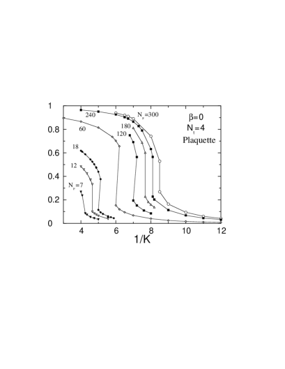
b)

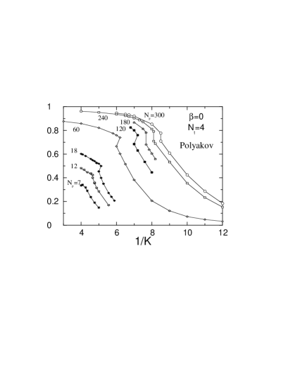
Figure 7: Plaquette (a) and Polyakov loop (b) at $\beta=0$ as a function of $1/K$ for various $N_{F}$ on $N_{t}=4$ lattices. Lines are to guide the eyes. In this figure, approximately vertical lines leaning to the right mean that we have two state signals there.

a)

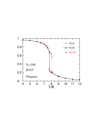
b)

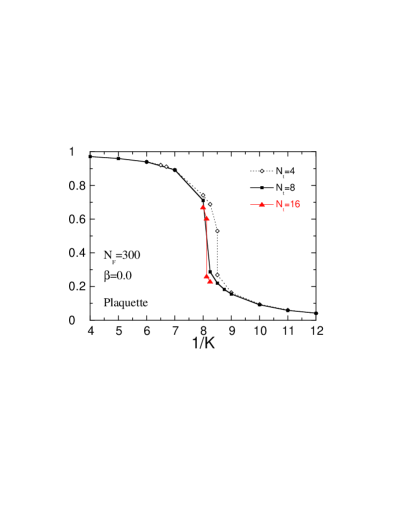
Figure 8: The plaquette at $\beta=0$ as a function of $1/K$ for (a) $N_{F}=240$ and (b) $N_{F}=300$, at $N_{t}=4$, 8 and 16. Lines are to guide the eyes.

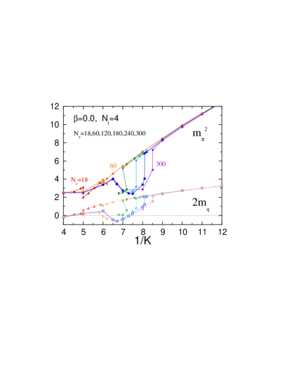
Figure 9: Results of $m_{\pi}^{2}$ and $2m_{q}$ at $\beta=0$ for $N_{F}=18$–300.

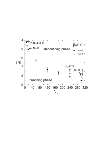
Figure 10: The transition point $1/K_{d}$ at $\beta=0$ versus $N_{F}$ for $N_{t}=4$ and $N_{t}\geq 8$. For clarity, data at $N_{t}=8$ for $N_{F}=300$ is slightly shifted to a larger $N_{F}$ in the figure.

VII Results of numerical simulations at $g=\infty$

We first study the strong coupling limit $\beta=0$ ($g=\infty$). In a previous work previo we have shown the following. When $N_{F}\leq 6$, we have only one confined phase from the heavy quark limit $K=0$ up to the chiral limit $K_{c}=0.25$. On the other hand, for $N_{F}\geq 7$, we found a strong first order transition at $K=K_{d}<K_{c}$. We confirmed that this transition $K_{d}$ is a bulk phase transition (transition at zero-temperature) by increasing the value of $N_{t}$ up to $N_{t}=18$ for $N_{F}=7$. When quarks are heavy ($K<K_{d}$), both the plaquette and the Polyakov loop are small, and $m_{\pi}$ satisfies the PCAC relation $m_{\pi}^{2}\propto m_{q}$. Therefore quarks are confined and the chiral symmetry is spontaneously broken in this phase. We found that $m_{q}$ in the confined phase is non-zero at the transition point $K_{d}$, i.e., the chiral limit does not belong to this phase. On the other hand, when quarks are light ($K>K_{d}$), the plaquette and the Polyakov loop are large. In this phase, $m_{\pi}$ remains large in the chiral limit and is almost equal to twice the lowest Matsubara frequency $\pi/N_{t}$. This implies that the pion state is an almost free two-quark state and, therefore, quarks are not confined in this phase. The pion mass is nearly equal to the scalar meson mass, and the rho meson mass to the axial vector meson mass. The chiral symmetry is also manifest within corrections due to finite lattice spacing.

In this paper, we extend the study to larger $N_{F}$. In Fig. 7, we show the results of the plaquette and Polyakov loop at $N_{t}=4$ for $N_{F}=7$ – 300. Clear first order transitions can be seen at $1/K$ larger than $1/0.25=4$. We then study the $N_{t}$ dependence of the results, as shown in Fig. 8 for the cases $N_{F}=240$ and 300. We find that, although the transition point shows a slight shift to smaller $1/K$ when we increase $N_{t}$ from 4 to 8, the transition stays at the same point for $N_{t}\geq 8$. For $N_{F}=240$, $1/K_{d}\simeq 8.1(1)$ at $N_{t}=4$ and $1/K_{d}=7.8(2)$ at $N_{t}=8$ and 16. A similar result was reported for $N_{F}=7$ in previo . We conclude that the transition is a bulk transition for $N_{F}\geq 7$.

Figure 9 shows the results of $m_{\pi}^{2}$ and $2m_{q}$, in the lattice units, at $\beta=0$ for various numbers of flavors. We clearly see that at the exactly same hopping parameter $K=K_{d}$ where the plaquette makes a gap, the pion mass and the quark mass also make gaps. When the quark is heavy ($K\leq K_{d}$), the PCAC relation ($m_{\pi}^{2}\propto m_{q}$) is well satisfied. On the other hand, when the quark mass is smaller than the critical value, the $1/K$ dependence of the pion mass squared $m_{\pi}^{2}$ and the quark mass $m_{q}$ looks strange at first sight. However, when one compares this dependence of $m_{q}$ with that of the free quark case shown in Fig. 3(a), one easily notices that the $1/K$ dependence is essentially the same as that of the free quark. The quark mass vanishes at $1/K\simeq 7$–8 for $N_{F}=60$, 240, and 300. This corresponds to the fact that the free quark mass vanishes at $1/K=8$. The $1/K$ dependence of $m_{\pi}^{2}$ is also essentially the same as that of the free quark case shown in Fig. 3(b). We stress that the chiral limit where the quark mass vanishes does not exist in the confined phase.

We show a map of the phase transition point $K=K_{d}$ at $\beta=0$ in Fig. 10.

a)

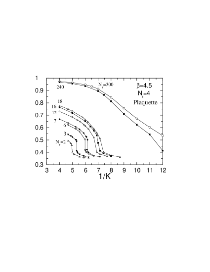
b)

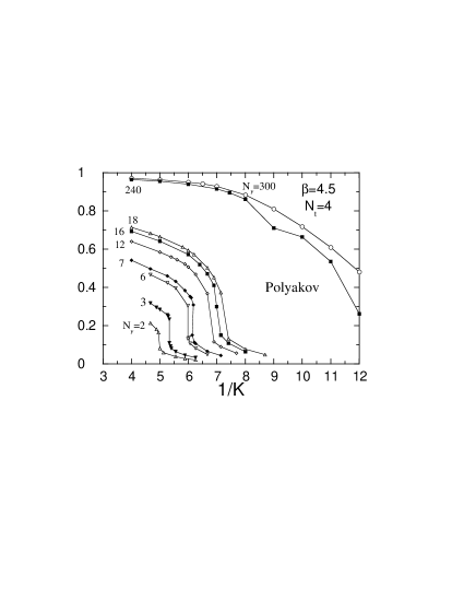
Figure 11: Results of (a) plaquette and (b) Polyakov loop for various $N_{F}$ obtained at $\beta=4.5$ on $N_{t}=4$ lattices.

a)

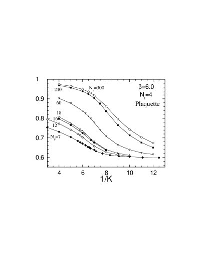
b)

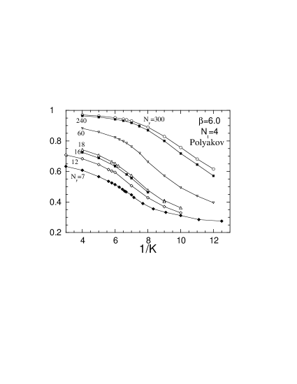
Figure 12: The same as Fig. 11, but for $\beta=6.0$.

a)

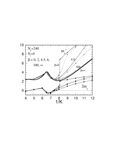
b)

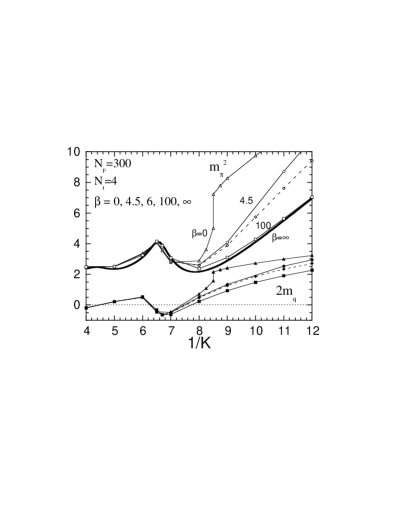
Figure 13: $m_{\pi}^{2}$ and 2$m_{q}$ for (a) $N_{F}=240$ and (b) 300, obtained on $N_{t}=4$ lattices at various $\beta$.

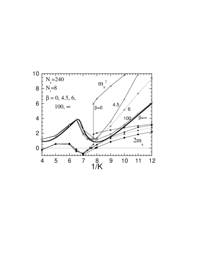
Figure 14: The same as Fig. 13, but for $N_{F}=240$ and $N_{t}=8$.

a)

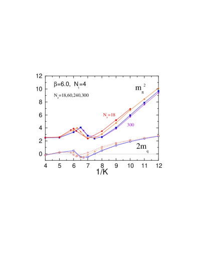
b)

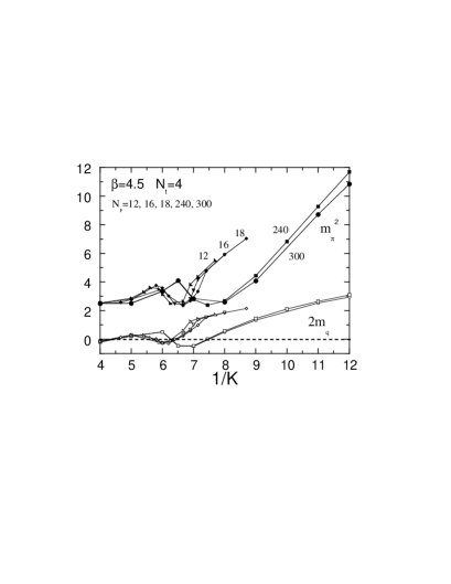
Figure 15: Results of $m_{\pi}^{2}$ and 2$m_{q}$ for large $N_{F}$ obtained on $N_{t}=4$ lattices at (a) $\beta=6.0$ and (b) $\beta=4.5$.

a)

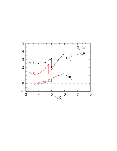
b)

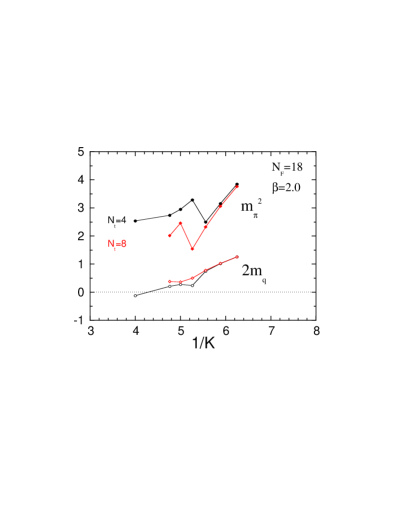
Figure 16: $N_{F}=18$: Results of $m_{\pi}^{2}$ and 2$m_{q}$ versus $1/K$. (a) $\beta=0.0$ and (b) $\beta=2.0$,

a)

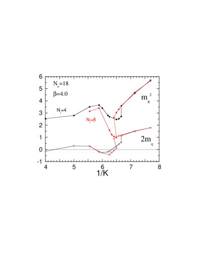
b)

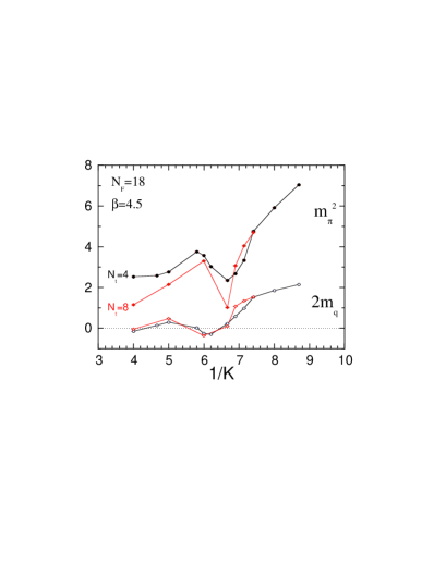
c)

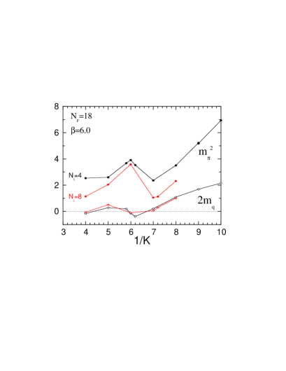
Figure 17: $N_{F}=18$: Results of $m_{\pi}^{2}$ and 2$m_{q}$ versus $1/K$. (a) $\beta=4.0$, (b) $\beta=4.5$, and (c) $\beta=6.0$.

a)

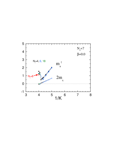
b)

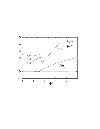
Figure 18: $N_{F}=7$: Results of $m_{\pi}^{2}$ and 2$m_{q}$ versus $1/K$. (a) $\beta=0.0$, (b) $\beta=2.0$.

a)

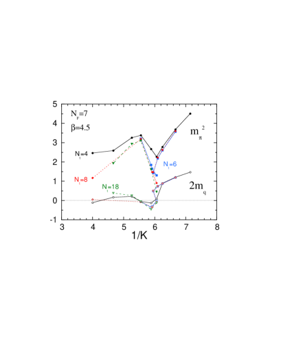
b)

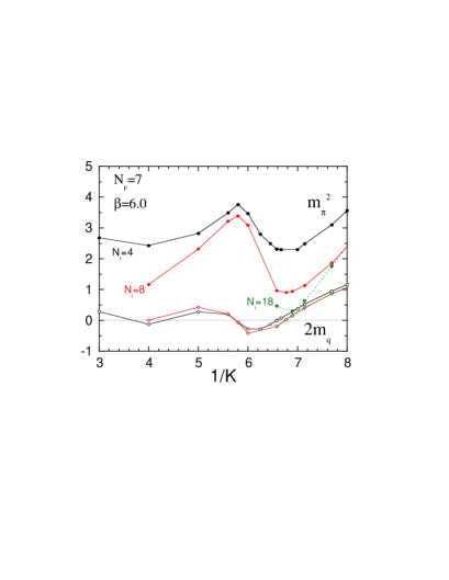
Figure 19: $N_{F}=7$: Results of $m_{\pi}^{2}$ and 2$m_{q}$ versus $1/K$. (a) $\beta=4.5$, (b) $\beta=6.0$.

a)

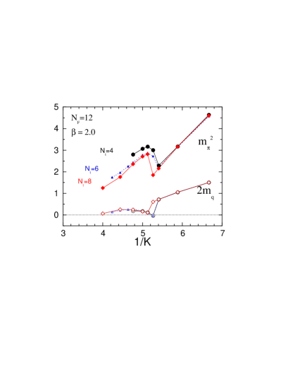
b)

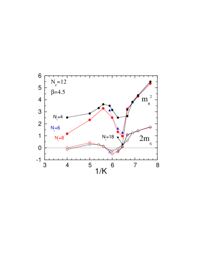
Figure 20: $N_{F}=12$: Results of $m_{\pi}^{2}$ and 2$m_{q}$ versus $1/K$. (a) $\beta=2.0$, (b) $\beta=4.5$.

a)

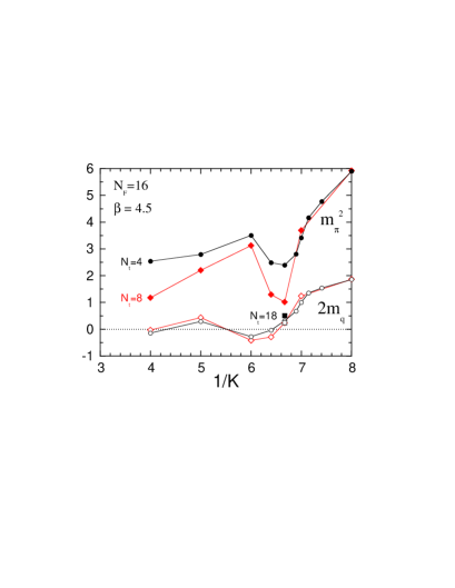
b)

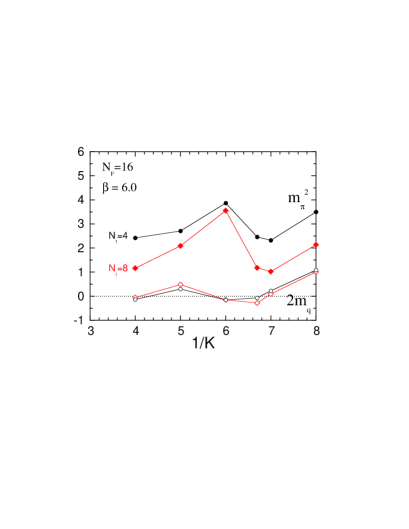
Figure 21: $N_{F}=16$: Results of $m_{\pi}^{2}$ and 2$m_{q}$ versus $1/K$. (a) $\beta=4.5$, (b) $\beta=6.0$.

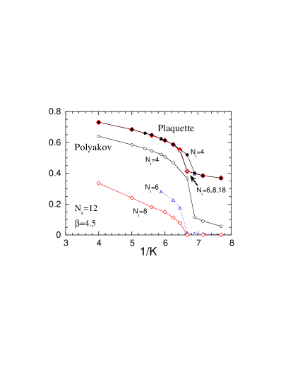
Figure 22: $N_{F}=12$: Plaquette and Polyakov loop as functions of $1/K$ and $N_{t}$ at $\beta=4.5$.

VIII Results of numerical simulations at finite $g$

We now extend the study to finite $\beta$ ($g<\infty$). Results of the plaquette and Polyakov loops at $\beta=4.5$ and 6.0 are plotted in Figs. 11 and 12, respectively, for various $N_{F}$. We note that at $\beta=4.5$, both the plaquette and Polyakov loop shows singular behavior at some quark mass for $N_{F}\leq 18$, in contrast to the cases of $N_{F}\geq 240$.

In order to understand the structure of the phase diagram for each number of flavors, from now on we discuss each $N_{F}$ separately: We first intensively investigate the cases $N_{F}=240$ and 300, and then decrease $N_{F}$, because we found that the phase structure is quite simple for $N_{F}$ $>$$\sim$ 240.

VIII.1 $N_{F}=240$ and $300$

Figure 13 shows the results of $m_{\pi}^{2}$ and $2m_{q}$ for $N_{F}=240$ and 300, obtained at various values of $\beta$ on the $N_{t}=4$ lattice. A very striking fact is that the shape of $m_{\pi}^{2}$ and $2m_{q}$ as a function of $1/K$ only slightly changes in the deconfined phase, when the value of $\beta$ decreases from $\infty$ down 0. Only the position of the local minimum of $m_{\pi}^{2}$ at $1/K\simeq 8$, which corresponds to the vanishing point of $m_{q}$, slightly shifts toward smaller $1/K$. The results for $N_{F}=240$ and 300 are essentially the same, except for very small shifts of the transition point and the minimum point of $m_{\pi}^{2}$. We obtain similar results also for $N_{t}=8$ (see Fig. 14). That is, the massless line in the deconfined phase runs through from $\beta=\infty$ to $\beta=0$. Thus we obtain the phase diagram shown in Fig. 5.

From the perturbation theory, the $m_{q}=0$ point at $\beta=\infty$ is a trivial IR fixed point for $N_{F}\geq 17$. The phase diagram shown in Fig. 5 suggests that there are no other fixed points on the $m_{q}=0$ line at finite $\beta$. In order to confirm this, we investigate the direction of the renormalization group (RG) flow along the $m_{q}=0$ line for $N_{F}=240$, using a Monte Carlo renormalization group (MCRG) method.

We make a block transformation for a change of scale factor 2, and estimate the quantity $\Delta\beta=\beta(2a)-\beta(a)$: We generate configurations on an $8^{4}$ lattice on the $m_{q}=0$ points at $\beta=0$ and 6.0 and make twice blockings. We also generate configurations on a $4^{4}$ lattice and make once a blocking. Then we calculate $\Delta\beta$ by matching the value of the plaquette at each step. From a matching of our data, we obtain $\Delta\beta\simeq 6.5$ at $\beta=0$ and $10.5$ at $\beta=6.0$. The value obtained from the two-loop perturbation theory is $\Delta\beta\simeq 8.8$ at $\beta=6.0$. The signs are the same and the magnitudes are comparable.

It is known for the pure SU(3) gauge theory that one has to make a more careful analysis using several types of Wilson loop with many blocking steps to extract a precise value of $\Delta\beta$. We reserve elaboration of this point and a fine tuning of $1/K$ at each $\beta$ for future works. For $N_{F}=240$, because the velocity of the RG flow is large, we will be able to obtain the sign and an approximate value of $\Delta\beta$ by a simple matching.

This result implies that the direction of the RG flow on the $m_{q}=0$ line at $\beta=0$ and 6.0 is the same as that at $\beta=\infty$. This further suggests that there are no fixed points at finite $\beta$. All of the above imply that the theory is trivial for $N_{F}=240$.

VIII.2 $240>N_{F}\geq 17$

Now we decrease $N_{F}$ from 240. As discussed in Sec. VII, the deconfined phase transition point $K_{d}$ decreases with decreasing $N_{F}$ in the strong coupling limit $\beta=0$. However, except for this shift of the bulk transition point, the $1/K$ dependence of $m_{\pi}^{2}$ and $m_{q}$ are quite similar in the deconfined phase when we vary $N_{F}$ from 300 down to 17, as shown in Fig. 9. The results at $\beta=6.0$ and 4.5 shown in Fig. 15 indicate that the $1/K$ dependence of $m_{\pi}^{2}$ and $m_{q}$ are almost identical to each other, except for a small shift toward smaller $1/K$ as $N_{F}$ is decreased. These facts imply that the structures of the deconfined phase are essentially identical from $N_{F}=17$ to 300.

As we show below, a closer examination of the data shows that the massless quark line in the deconfined phase hits the phase transition line at finite $\beta$ when $N_{F}$ is not so large as $N_{F}\leq 60$, while it runs through from $\beta=\infty$ to $\beta=0$ when $N_{F}$ is very large such as 240 and 300.

For $N_{F}=18$ we make simulations at $\beta=0.0$, 2.0, 4.0, 4.5, and 6.0 on $N_{t}=4$ and 8 lattices, as listed in Table 6. Results for $m_{\pi}^{2}$ and $m_{q}$ are shown in Figs. 16 and 17. We note that, at $\beta=4.5$, the $m_{\pi}^{2}$ and $m_{q}$ show characteristic behavior of massless quarks around $1/K=6.5$ in the deconfined phase, both on $N_{t}=4$ and 8 lattices. Such massless point exists also at $\beta=6.0$, but is absent at $\beta=0.0$ and 2.0.

At $\beta=4.0$ we carry out detailed simulations around the transition point. On the $N_{t}=4$ lattice, the first order deconfining phase transition locates around $K=0.150$ ($1/K=6.67$), and the massless quark point exists at $K\simeq 0.158$ ($1/K\simeq 6.33$) in the deconfined phase. When we increase $N_{t}$ to 8, the phase transition point shifts to $K=0.154$–0.156 ($1/K=6.49$–6.41) where we observe two-state signals lasting more than 450 trajectories. We confirm that the points $K=0.152$ and 0.158 belong to the confined and deconfined phase, respectively. In the deconfined phase the massless quark point exists at $K\simeq 0.155$ ($1/K\simeq 6.45$). See Fig. 17(a). From this we conclude that the massless quark line in the deconfined phase hits the first order bulk phase transition line around $\beta=4.0$. The phase structure for $N_{F}=18$ is summarized in Fig. 6(a).

VIII.3 $16\geq N_{F}\geq 7$

As stressed several times, the quark confinement is lost for $N_{F}\geq 7$ at $\beta=0$ ($g=\infty$). We now intensively simulate the cases $N_{F}=7$, 12 and 16 at several finite values of $\beta$. The simulation parameters for $N_{F}=7$, 12 and 16 are listed in Tables 2, 4 and 5.

In Figs. 18 and 19, $m_{\pi}^{2}$ and $2m_{q}$ at selected values of $\beta$ are plotted for $N_{F}=7$. Results for $N_{F}=12$ and 16 are similar, as shown in Figs. 20 and 21.

For $N_{F}=7$, 12 and 16, we find that the $1/K$ dependence of $m_{\pi}^{2}$ and $2m_{q}$ in the deconfined phase are similar to those shown in Fig. 15 for $N_{F}\geq 17$ at all the values of $\beta$. That is, they are essentially the same as those of a free quark state shown in Fig. 3. Careful looking at the values of $m_{\pi}^{2}$ and $2m_{q}$ at $\beta=4.5$ for both cases reveals that the massless line hits the phase transition line around $\beta=4.5$, at $1/K\sim 6.1$ for $N_{F}=7$ and at $1/K\sim 6.5$ for $N_{F}=12$.

Together with the data of plaquette and Polyakov loop (see Fig. 22 as a typical example), we obtain the phase diagram shown in Fig. 6(b) for $N_{F}=12$. The phase diagrams for $N_{F}=7$ and 16 are similar. We find that the gross feature of these phase diagrams is quite similar to the case $N_{F}=18$ shown in Fig. 6(a).

We note again that when $N_{F}\leq 16$, the point $g=0$ is an UV fixed point. This is in clear difference with the case of $N_{F}\geq 17$.

VIII.4 $N_{F}\leq 6$

As already reported in ref. previo , numerical results show that, at $\beta=0$, the confined phase extends to the chiral limit. Simulations at finite values of $\beta$ show that the phase structure is similar for $N_{F}=2$–6 Stand26 . (See Table 1 for run parameters for $N_{F}=6$.) Thus we have the phase diagram shown in Fig. 4.

IX Implication for physics

We now extend the discussion to the cases of non-degenerate quarks. In the case of degenerate masses, the global structure of the phase diagram is the same at large $\beta$ for $N_{F}\geq 7$. As far as the quark mass is below a critical value, the system is in the deconfined phase. Therefore, we expect that our proposal for the relation of the phase structure and the number of flavors remain unchanged for non-degenerate cases, when we redefine $N_{F}$ as the number of flavors which satisfies the condition $m_{0}<\Lambda_{d}$: If there exist more than seven quarks whose masses are lighter than $\Lambda_{d}$, quarks should not be confined. In nature quarks are confined, therefore the number of flavors whose masses are less than $\Lambda_{d}$ should be equal or less than six. The scale $\Lambda_{d}$ is numerically calculable and will be obtained in the future.

This conclusion is based on our assumption that the deconfining phase transition occurs at $m_{0}^{critical}\sim\xi^{-1}$. Now we make a comment on the alternative possibility that the deconfining phase transition occurs at $m_{0}^{critical}\sim a^{-1}$. If this would be correct, the number of flavors should be equal or less than six irrespective of their masses. Since six species of quarks have been discovered, this implies that there are no more species of quarks.

X Conclusions

We have investigated numerically the phase structure of QCD for the general number of flavors. Performing a series of simulations for degenerate quark mass cases employing the one-plaquette gauge action and the standard Wilson quark action, we have found that when $N_{F}\geq 7$ there is a line of a first order phase transition between the confined phase and a deconfined phase at a finite current quark mass in the strong coupling region and the intermediate coupling region. The massless quark line exists only in the deconfined phase.

Based on these numerical results in the strong coupling limit and in the intermediate coupling region, together with an assumption that the phase transition occurs at $m_{0}^{critical}\sim\xi^{-1}$ in the weak coupling region, where $\xi$ is a typical correlation length of gluons, we propose the following phase structure. The phase structure crucially depends on the number of flavors, $N_{F}$, whose masses are less than $\Lambda_{d}\sim\xi^{-1}$ which is the physical scale which characterizes the phase transition: When $N_{F}\geq 17$, there is only a trivial IR fixed point and therefore the theory in the continuum limit is free. On the other hand, when $16\geq N_{F}\geq 7$, there is a non-trivial IR fixed point and therefore the theory is non-trivial with anomalous dimensions, however, without quark confinement. Theories which satisfy both quark confinement and spontaneous chiral symmetry breaking in the continuum limit exist only for $N_{F}\leq 6$. If there exist more than seven quarks whose masses are lighter than $\Lambda_{d}$, quarks should not be confined. In nature quarks are confined, therefore the number of flavors whose masses are less than $\Lambda_{d}$ should be equal or less than six. The scale $\Lambda_{d}$ is numerically calculable and will be obtained in the future.

We have discussed that, only from a theoretical argument, we cannot exclude an alternative possibility that the deconfining phase transition occurs at $m_{0}^{critical}\sim a^{-1}$. This corresponds to the case $\Lambda_{d}=\infty$. If this would be correct, the total number of flavors should be equal or less than six irrespective of their masses: Since six species of quarks have been discovered, this implies that there are no more species of quarks. This conclusions is based on an additional assumption that QCD only is responsible to quark confinement. If some other interactions would also affect the quark confinement at some scale $\Lambda_{new}$, the number of quarks, whose masses are smaller than $\Lambda_{new}$, should be six, in this case.

Which of $m_{0}^{critical}\sim a^{-1}$ or $m_{0}^{critical}\sim\xi^{-1}$ is realized can be investigated by numerical simulations in future.

Appendix: SU(2) QCD

a)

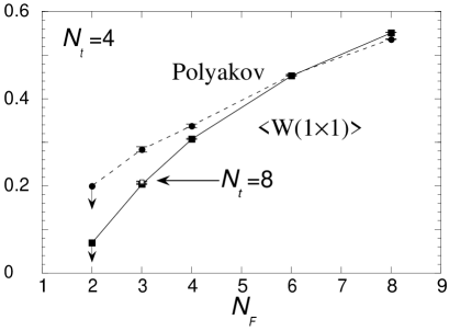
b)

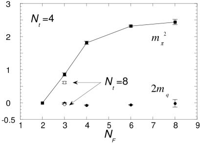
Figure 23: Results of physical quantities at $g=\infty$ and $K=K_{c}$ for SU(2) QCD. (a) the plaquette and Polyakov loop, and (b) $m_{\pi}^{2}$ and 2$m_{q}$.

Table 10: Simulation parameters for SU(2) QCD at $\beta=0.0$ performed on $8^{2}\times 10\times N_{t}$ lattices with $N_{t}=4$ and 8. The number of configurations, sampled every 5 trajectories, are 10–22, except for the $N_{F}=2$ runs at $K=0.25$ which are not thermalized.

$N_{F}$	$N_{t}$	$\kappa$	$\Delta\tau$
2	4	0.25	0.01, 0.005
3	4	0.21, 0.22, 0.23, 0.24, 0.25	0.01
	8	0.25	0.01
4	4	0.25	0.01
6	4	0.25	0.01
8	4	0.16, 0.17, 0.18, 0.19, 0.20,
		0.21, 0.23, 0.25	0.01

As an extension of the color SU(3) QCD case, we study color SU(2) QCD in the strong coupling limit. We note that the SU(2) beta function has a characteristics similar to the SU(3) one: In the case of SU(2), the asymptotic freedom is lost when $N_{F}\geq 11$ and the 2-loop result for the critical $N_{F}$ is 5, instead of 17 and 8, respectively, for SU(3) previo . The smaller numbers for critical $N_{F}$ are natural because the confining force is weaker in SU(2).

Adopting the standard plaquette gauge action and the Wilson quark action, we have performed a series of simulations in the strong coupling limit following the strategy of the SU(3) case. Our simulation parameters are compiled in Table 10.

First, performing a simulation for $N_{F}=8$ and $N_{t}=4$, we confirm that the deconfining transition occurs at $K=0.2$–0.21 and that the chiral limit $K=K_{c}=0.25$ is in the deconfined phase. Decreasing $N_{F}$ gradually at $K=K_{c}$, we find that the chiral limit remains in the deconfined phase down to $N_{F}=3$. When we further decrease $N_{F}$ to 2, the number of the inversion $N_{inv}$ in CG iterations shows a rapid increase with molecular-dynamics time and finally exceeds 10,000 in clear contrast with small numbers of $O(10^{2})$ for $N_{F}\geq 3$. We conclude that the chiral limit is in the confined phase for $N_{F}=2$. Fig. 23(a) shows our results of physical quantities versus $N_{F}$ at $K=K_{c}$. To study the $N_{t}$ dependence of the transition, we simulate on an $N_{t}=8$ lattice for the critical case $N_{F}=3$. The stability of the result, shown in Fig. 23(b), confirms that the deconfining transition we observe is a bulk phase transition.

At finite coupling constants we may expect results similar to those of SU(3). Thus, we conjecture in parallel to the SU(3) case that, when $N_{F}\geq 11$, the theory is free. On the other hand, when $10\geq N_{F}\geq 3$, the theory is non-trivial with anomalous dimensions without quark confinement. Theories which satisfies both quark confinement and spontaneous chiral symmetry breaking exists only for $N_{F}\leq 2$.

References

- (1) Y. Iwasaki, K. Kanaya, S. Sakai, and T. Yoshié, Phys. Rev. Lett. 69 (1992) 21.
- (2) Y. Iwasaki, K. Kanaya, S. Sakai, and T. Yoshié, Nucl. Phys. B(Proc. Suppl.) 30 (1993), 327; Y. Iwasaki, K. Kanaya, S. Sakai, and T. Yoshié, Nucl. Phys. B(Proc. Suppl.) 34 (1994), 314. Y. Iwasaki, K. Kanaya, S. Kaya, S. Sakai, and T. Yoshié, Nucl. Phys. B (Proc. Suppl.) 53 (1997) 449.
- (3) Y. Iwasaki, in “Perspectives of Strong Coupling Gauge Theories”, eds. J. Nishimura and K. Yamawaki, World Sci. (1997) 135–149 [Proc. International Workshop SCGT96, Nov. 13-16, 1996, Nagoya, Japan]. Y. Iwasaki, K. Kanaya, S. Kaya, S. Sakai, and T. Yoshié, Prog. Theor. Phys. Suppl. 131 (1998) 415. Y. Iwasaki, K. Kanaya, S. Kaya, T. Yoshié and S. Sakai, in “Dynamics of Gauge Fields”, eds. A. Chodos, et al., Universal Academy Press (2000) 145–158 [Proc. TMU-Yale Symposium, Dec.13–15, 1999, Hachioji, Japan]. Y. Iwasaki, in Proc. International Workshop SCGT2002, Nagoya, Dec. 10-13, 2002.
- (4) T. Banks and A. Zaks, Nucl. Phys. B196 (1982) 189.
- (5) J. Kogut, R. Pearson and J. Shigemitsu, Phys. Rev. Lett. 43 (1979) 484.
- (6) H. Kluberg-Stern , A. Morel, O. Napoly and B. Petersson, Nucl. Phys. B190 [FS3] (1981) 504. N. Kawamoto, Nucl. Phys. B190 [FS3] (1981) 617. N. Kawamoto and J. Smit, Nucl. Phys. B192 (1981) 100.
- (7) J. Smit, Nucl. Phys. B175 (1980) 307. J. Greensite and J. Primack, Nucl. Phys. B180 [FS2] (1981) 170. H. Kluberg-Stern, A. Morel and B. Petersson, Nucl. Phys. B215 [FS7] (1983) 527.
- (8) J.-M. Blairon, R. Brout, F. Englert and J. Greensite, Nucl. Phys. B180 [FS2] (1981) 439.
- (9) K. Wilson, in “New Phenomena in Subnuclear Physics” (Erice 1975), ed. A. Zichichi (Plenum, New York, 1977).
- (10) R. Oehme and W. Zimmermann, Phys. Rev. D21 (1980) 471; 1661. R. Oehme, Phys. Rev. D42 (1990) 4209.
- (11) K. Nishijima, Nucl. Phys. B238 (1984) 601; Prog. Theor. Phys. 75 (1986) 22; Prog. Theor. Phys. 77 (1987) 1053.
- (12) T. Appelquist et al., Phys. Rev. Lett. 77 (1996) 1214. V.A. Miransky and K. Yamawaki, Phys. Rev. D55 (1997) 5051, erratum D56 (1997) 3768. T. Appelquist et al., Phys. Rev. D58 (1998) 105017.
- (13) R.D. Pisarski and D.L. Stein, Phys. Rev. B23 (1981) 3549; J. Phys. A14 (1981) 3341. A.J. Paterson, Nucl. Phys. B190 [FS3] (1981) 188.
- (14) Y. Iwasaki, K. Kanaya, S. Kaya, S. Sakai, and T. Yoshié, Phys. Rev. D54 (1996) 7010.
- (15) M. Bochicchio et al., Nucl. Phys. B262 (1985) 331.
- (16) S. Itoh, Y. Iwasaki, Y. Oyanagi and T. Yoshié, Nucl. Phys. B274 (1986) 33.
- (17) Y. Iwasaki, K. Kanaya, S. Sakai, and T. Yoshié, Phys. Rev. Lett. 69 (1992) 21.
- (18) Y. Iwasaki et al., Phys. Rev. D46 (1992) 4657.
- (19) G. Boyd et al., Nucl. Phys. B469 (1996) 419.
- (20) S. Aoki, Phys. Rev. D30 (1984) 2653; S. Aoki, A. Ukawa and T. Umeda, Phys. Rev. Lett. 76 (1996) 873.
- (21) S. Gottlieb, W. Liu, D. Toussaint, R.L. Renken and R.L. Sugar, Phys. Rev. D35 (1987) 2531.
- (22) J. Kogut and L. Susskind, Phys. Rev. D11 (1975) 395. L. Susskind, Phys. Rev. D16 (1977) 3031.
- (23) J.B. Kogut, J. Polonyi, H.W. Wyld and D.K. Sinclair, Phys. Rev. Lett. 14 (1985) 1475. R.V. Gavai, Nucl. Phys. B269 (1986) 530. N. Attig, B. Petersson, M. Wolff, Phys. Lett. bf B190 (1987) 143.
- (24) J.B. Kogut and D.K. Sinclair, Nucl. Phys. B295 [FS21] (1988) 465.
- (25) M. Fukugita, S. Ohta and A. Ukawa, Phys. Rev. Lett. 60 (1988) 178.
- (26) S. Ohta and S. Kim, Phys. Rev. D44 (1991) 504. S. Kim and S. Ohta. Nucl. Phys. B (Proc. Suppl.) 106 & 107 (2002) 873.
- (27) F. Brown et al., Phys. Rev. D46 (1992) 5655.
- (28) P.H. Damgaard, U.M. Heller, A. Krasnitz and P. Olesen, Phys. Lett. B400 (1997) 169.
- (29) Y. Iwasaki, K. Kanaya, S. Sakai, and T. Yoshié, Z. Phys. C71 (1996) 337; Y. Iwasaki, K. Kanaya, S. Kaya, S. Sakai, and T. Yoshié, ibid. C71 (1996) 3343.