Maximum Entropy Method Approach to the $\theta$ Term

Abstract

In Monte Carlo simulations of lattice field theory with a $\theta$ term, one confronts the complex weight problem, or the sign problem. This is circumvented by performing the Fourier transform of the topological charge distribution $P(Q)$. This procedure, however, causes flattening phenomenon of the free energy $f(\theta)$, which makes study of the phase structure unfeasible. In order to treat this problem, we apply the maximum entropy method (MEM) to a Gaussian form of $P(Q)$, which serves as a good example to test whether the MEM can be applied effectively to the $\theta$ term. We study the case with flattening as well as that without flattening. In the latter case, the results of the MEM agree with those obtained from the direct application of the Fourier transform. For the former, the MEM gives a smoother $f(\theta)$ than that of the Fourier transform. Among various default models investigated, the images which yield the least error do not show flattening, although some others cannot be excluded given the uncertainty related to statistical error.

1 Introduction

It is believed that the $\theta$ term could affect the dynamics at low energy and the vacuum structure of QCD, but it is known from experimental evidence that the value of $\theta$ is strongly suppressed in Nature. From the theoretical point of view, the reason for this is not clear yet. Hence, it is important to study the properties of QCD with the $\theta$ term to clarify the structure of the QCD vacuum. [1]   For theories with the $\theta$ term, it has been pointed out that rich phase structures could be realized in $\theta$ space. For example, the phase structure of the $Z(N)$ gauge model was investigated using free energy arguments, and it was found that oblique confinement phases could occur. [2]  In CP^N-1 models, which have several dynamical properties in common with QCD, it has been shown that a first-order phase transition exists at $\theta=\pi$ [3, 4, 5].

Although numerical simulation is one of the most effective tools to study non-perturbative properties of field theories, the introduction of the $\theta$ term makes the Boltzmann weight complex. This makes it difficult to perform Monte Carlo (MC) simulations on a Euclidean lattice. This is the complex action problem, or the sign problem. In order to circumvent this problem, the following method is conventionally employed. [6, 7]   The partition function ${\cal Z}(\theta)$ can be obtained by Fourier-transforming the topological charge distribution $P(Q)$, which is calculated with a real positive Boltzmann weight:

$${\cal Z}(\theta)=\frac{\int[d\bar{z}dz]e^{-S+i\theta\hat{Q}(\bar{z},z)}}{\int[d\bar{z}dz]e^{-S}}\equiv\sum_{Q}e^{i\theta Q}P(Q),$$ (1)

where

$$P(Q)\equiv\frac{\int[d\bar{z}dz]_{Q}e^{-S}}{\int d\bar{z}dze^{-S}}.$$ (2)

The measure $[d\bar{z}dz]_{Q}$ in Eq. (2) is such that the integral is restricted to configurations of the field $z$ with topological charge $Q$. Also, $S$ represents the action.

In the study of CP^N-1 models, it is known that this algorithm works well for a small lattice volume $V$ and in the strong coupling region [6, 4, 8, 9].  As the volume increases or in the weak coupling region, however, this strategy too suffers from the sign problem for $\theta\simeq\pi$. The error in $P(Q)$ masks the true values of ${\cal Z}(\theta)$ in the vicinity of $\theta=\pi$, and this results in a fictitious signal of a phase transition [10].   This is called ‘flattening’, because the free energy becomes almost flat for $\theta$ larger than a certain value. This problem could be remedied by reducing the error in $P(Q)$. This, however, is hopeless, because the amount of data needed to reduce the error to a given level increases exponentially with $V$. Recently, an alternative method has been proposed to circumvent the sign problem. [11, 12]

Our aim in the present paper is to reconsider this problem from the point of view of the maximum entropy method (MEM) [13, 14, 15, 16, 17].   The MEM is well known as a powerful tool for so-called ill-posed problems, where the number of parameters to be determined is much larger than the number of data points. It has been applied to a wide range of fields, such as radio astrophysics and condensed matter physics. Recently, spectral functions in lattice field theory have been widely studied by use of the MEM [17, 18, 19, 20].  In the present paper, we are interested in whether the MEM can be applied effectively to the study of the $\theta$ term and to what extent one can improve the flattening phenomenon of the free energy.

The MEM is based upon Bayes’ theorem. It derives the most probable parameters by utilizing data sets and our knowledge about these parameters in terms of the probability. The probability distribution, which is called the posterior probability, is given by the product of the likelihood function and the prior probability. The latter is represented by the Shannon-Jaynes entropy, which plays an important role to guarantee the uniqueness of the solution, and the former is given by $\chi^{2}$. It should be noted that artificial assumptions are not needed in the calculations, because the determination of a unique solution is carried out according to probability theory. Our task is to determine the image for which the posterior probability is maximized. In practice, however, it is difficult to find a unique solution in the huge configuration space of the image. In order to do so effectively, we employ the singular value decomposition (SVD).

The flattening of the free energy is an inherent phenomenon in the Fourier transformation procedure. It is quite independent of the models used. We choose a Gaussian form of $P(Q)$, which is realized in many cases, such as the strong coupling region of the CP^N-1 model and the 2-d U(1) gauge model. Because the Gaussian $P(Q)$ can be analytically Fourier-transformed to ${\cal Z}(\theta)$, it provides a good example to investigate whether the MEM would be effective. For the analysis, we use mock data by adding noise to $P(Q)$ in the cases with and without flattening. The most probable images of the partition function are obtained. The uncertainty of the images is used as an estimate of the error.

Our conclusion is summarized as follows.

1. In the case without flattening, the results of the MEM are consistent with those of the Fourier transformation and thus reproduce the exact results.

2. In the case with flattening, the MEM yields a smoother free energy density than the Fourier transform. Among various default models investigated, some images with the least errors do not exhibit flattening. With regard to the question of which is the best among such images, further consideration of the systematic error is needed to check the robustness of the images.

This paper is organized as follows. In the following section, we give an overview of the origin of flattening. In $\S$ 3, we summarize the procedure for the analysis of the MEM. The results obtained by use of the MEM are presented in $\S$ 4. A summary is given in $\S$ 5.

2 Sign problem and flattening behavior of the free energy

In this section, we briefly review the flattening phenomenon of the free energy density. It is observed when one employs an algorithm in which ${\cal Z}(\theta)$ is calculated through the Fourier transform. In order to obtain ${\cal Z}(\theta)$, we must calculate $P(Q)$ with high precision. Although $P(Q)$ is calculated over a wide range of orders by use of the set method [21],   the error in $P(Q)$ yields error in ${\cal Z}(\theta)$ through the Fourier transform. This effect becomes serious in the large $\theta$ region. Here, we use a Gaussian $P(Q)$ for our investigation. The Gaussian $P(Q)$ is not just a toy model, but indeed it is realized in a variety of models, such as the 2-d U(1) gauge model and in the strong coupling limit of CP^N-1 models.

We parameterize the Gaussian $P(Q)$ as

$$P(Q)=A\exp[-\frac{c}{V}Q^{2}],$$ (3)

where, in the case of the 2-d U(1) gauge model, $c$ is a constant depending on the inverse coupling constant $\beta$, and $V$ is the lattice volume. Hereafter, $V$ is regarded as a parameter and varied in the analysis. The constant $A$ is fixed so that $\sum_{Q}P(Q)=1$. The distribution $P(Q)$ is analytically transformed by use of the Poisson sum formula into the partition function

$${\cal Z}_{\rm pois}(\theta)=A\sqrt{\frac{\pi V}{c}}\sum_{n=-\infty}^{\infty}\exp\biggl{[}-\frac{V}{4c}(\theta-2\pi n)^{2}\biggr{]}.$$ (4)

To prepare the mock data, we add noise with variance $\delta\times P(Q)$ to the Gaussian $P(Q)$. In the analysis, we consider sets of data with various values of $\delta$ and study the effects of $\delta$.

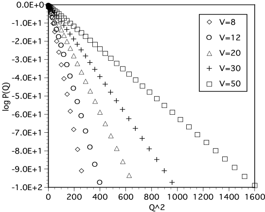
Figure 1: Gaussian topological charge distribution for various lattice volumes. The parameter $\delta$ is chosen to be 1/400.

Figure 1 displays the Gaussian $P(Q)$ for various lattice volumes $V$. The parameter $c$ is fixed at $c=7.42$. The corresponding free energy densities, $f(\theta)=-\frac{1}{V}\log{\cal Z}(\theta)$, calculated with Eq. (1), are plotted in Fig. 2. All functions $f(\theta)$ in Fig. 2 fall on a universal curve for $\theta\hskip 3.00003pt\raisebox{1.72218pt}{$<$}\raisebox{-3.01385pt}{$\sim$}\hskip 3.00003pt2.3$. For $\theta\hskip 3.00003pt\raisebox{1.72218pt}{$>$}\raisebox{-3.01385pt}{$\sim$}\hskip 3.00003pt2.3$, finite size effects are clearly observed. As the volume increases, $f(\theta)$ increases until $V\hskip 3.00003pt\raisebox{1.72218pt}{$<$}\raisebox{-3.01385pt}{$\sim$}\hskip 3.00003pt20$, but for $V=30$ and $V=50$, the Fourier transformation does not work . At $V=30$, ${\cal Z}(\theta)$ becomes negative for certain values of $\theta$, and at $V=50$, $f(\theta)$ becomes almost flat for $\theta\hskip 3.00003pt\raisebox{1.72218pt}{$>$}\raisebox{-3.01385pt}{$\sim$}\hskip 3.00003pt2.3$. The latter behavior causes a fictitious signal of a first-order phase transition at $\theta\approx 2.3$. The mechanism of this flattening [8, 5]  is briefly summarized as follows.

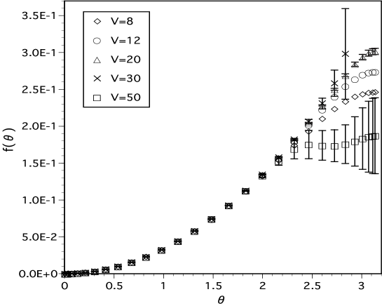
Figure 2: Free energy density $f(\theta)$ for various lattice volumes. $f(\theta)$ is calculated numerically by Fourier-transforming the Gaussian topological charge distribution.

The distribution $P(Q)$ obtained from MC simulations can be decomposed into two parts, a true value and an error:

$$P(Q)={\tilde{P}}(Q)+\Delta P(Q),$$ (5)

where $P(Q),\;{\tilde{P}}(Q)\;\mbox{and}\;\Delta P(Q)$ denote the MC data, the true value and the error, respectively. In order to calculate $P(Q)$ efficiently, which ranges over many orders, the set method and the trial function method are conventionally used. In the set method, the range of $Q$ is divided into several sets, each of which consists of several bins. In each set, the topological charge of the configurations is calculated in order to construct the histogram. The trial function method makes the distribution of the histogram almost flat. This is useful for reducing the error in $P(Q)$. Accordingly, the error is computed as [4]

$$\Delta P(Q)\sim\delta P(Q)\times P(Q),$$

where $\delta P(Q)$ is almost independent of $Q$. Because $P(Q)$ is a rapidly decreasing function, so is the statistical error $\Delta P(Q)$. Thus, the dominant contribution to $\Delta P(Q)$ comes from that at $Q=0$, and the partition function ${\cal Z}(\theta)$ has an error $\Delta P(0)\approx\delta P(0)P(0)\approx\delta P(0)$. The free energy density for the MC data is approximately given by

$$f(\theta) = -\frac{1}{V}\log{\cal Z}(\theta)\approx-\frac{1}{V}\log\Bigl{\{}\sum_{Q}{\tilde{P}}(Q)e^{i\theta Q}+\delta P(0)\Bigr{\}}$$ (6)

$$= -\frac{1}{V}\log\bigl{\{}e^{-V{\tilde{f}}(\theta)}+\delta P(0)\bigr{\}},$$

where ${\tilde{f}}(\theta)$ is the true free energy density. The value of $e^{-V{\tilde{f}}(\theta)}$ decreases rapidly as the volume $V$ and/or $\theta$ increase (see Fig. 2), and the magnitude of $e^{-V{\tilde{f}}(\theta)}$ becomes of order of $\delta P(0)$ at $\theta\simeq\theta_{\rm f}$. Therefore $f(\theta)$ cannot be calculated precisely, but $f(\theta)\simeq{\rm const.}$ for $\theta\hskip 3.00003pt\raisebox{1.72218pt}{$>$}\raisebox{-3.01385pt}{$\sim$}\hskip 3.00003pt\theta_{\rm f}$. This is the reason for the flattening behavior for $V=50$ in the region $\theta\hskip 3.00003pt\raisebox{1.72218pt}{$>$}\raisebox{-3.01385pt}{$\sim$}\hskip 3.00003pt\theta_{\rm f}\simeq 2.3$, as shown in Fig. 2. A drastic reduction of $\Delta P(Q)$ is necessary in order to properly estimate $f(\theta)$ for $\theta\hskip 3.00003pt\raisebox{1.72218pt}{$>$}\raisebox{-3.01385pt}{$\sim$}\hskip 3.00003pt\theta_{\rm f}$. In the case of a large volume, however, this is hopeless, because an exponentially increasing amount of data is needed. Therefore, we do need some other way to calculate $f(\theta)$.

3 MEM

In this section we briefly explain the concept of the MEM and the necessary procedures for the analysis in order to make this paper self-contained and to define the notation.

3.1 MEM based on Bayes’ theorem

In an experiment or a numerical simulation, data are always noisy, and the number of sets of data is finite. It is in principle impossible to reconstruct the true image from such data sets. Hence, it is reasonable to determine the most probable image. From Bayes’ theorem, the probability that an image ${\bf f}$ occurs for a given data set $\{{\bf D}\}$ is given by

$${\rm prob}({\bf f}|{\bf D})=\frac{{\rm prob}({\bf D}|{\bf f}){\rm prob}({\bf f})}{{\rm prob}({\bf D})},$$ (7)

where ${\rm prob}(A)$ is the probability that an event $A$ occurs and ${\rm prob}(A|B)$ is the conditional probability that $A$ occurs under the condition that $B$ occurs. Moreover, one can add to Eq. (7) ‘prior information’ $I$ about the image ${\bf f}$. The information $I$ includes that obtained from theoretical restrictions as well as knowledge based on previous experiments. With $I$, Eq. (7) becomes

$${\rm prob}({\bf f}|{\bf D},I)=\frac{{\rm prob}({\bf D}|{\bf f},I){\rm prob}({\bf f}|I)}{{\rm prob}({\bf D}|I)},$$ (8)

where ${\rm prob}(A,B)$ is the joint probability that events $A$ and $B$ occur simultaneously. The probability ${\rm prob}({\bf f}|{\bf D},I)$ is called the posterior probability. When the probability ${\rm prob}({\bf D}|{\bf f},I)$ is considered as a function of ${\bf f}$ for fixed data, it is equivalent to the likelihood function, which expresses how data points vary around the ‘true value’ corresponding to the true image ${\bf f}$. The probability ${\rm prob}({\bf f}|I)$ is called the prior probability and represents our state of knowledge about the image ${\bf f}$ before the experiment is carried out. The most probable image satisfies the condition

$$\frac{\delta~{}{\rm prob}({\bf f}|{\bf D},I)}{\delta\bf{f}}=0.$$ (9)

Recently, the MEM has been applied to hadronic spectral functions in lattice QCD. [17, 18]  In the analysis of the spectral function $A(\omega)$, the correlation function $D(\tau)$ is given by

$$D(\tau)=\int_{0}^{\infty}d\omega K(\tau,\omega)A(\omega),$$ (10)

where $K(\tau,\omega)$ denotes the kernel of the Laplace transform. In lattice theories, the number of data points is, at most, of order of $10-10^{2}$, due to the finite volume, while the number of the degrees of freedom to describe the continuous function $A(\omega)$ is in the range ${\cal O}(10^{2})-{\cal O}(10^{3})$.

Considering theories that include the $\theta$ term, what we have to deal with is

$$P(Q)=\int_{-\pi}^{\pi}d\theta\frac{e^{-i\theta Q}}{2\pi}{\cal Z}(\theta).$$ (11)

Comparing this with Eq. (10), we see the correspondence

$$\{P(Q)\leftrightarrow D(\tau),\;e^{-i\theta Q}/2\pi\leftrightarrow K(\tau,\omega),\;{\cal Z}(\theta)\leftrightarrow A(\omega)\};$$ (12)

that is, the continuous function ${\cal Z}(\theta)$ must be reconstructed from a finite number of data for $P(Q)$, which constitutes an ill-posed problem. Given this situation, what we would like to do in the present paper is to rely on the MEM, employing the formula

$${\rm prob}({\cal Z}(\theta)|P(Q),I)={\rm prob}({\cal Z}(\theta)|I)\frac{{\rm prob}(P(Q)|{\cal Z}(\theta),I)}{{\rm prob}(P(Q)|I)}.$$ (13)

The likelihood function ${\rm prob}(P(Q)|{\cal Z}(\theta),I)$ is given by

$${\rm prob}(P(Q)|{\cal Z}(\theta),I)=\frac{e^{-\frac{1}{2}\chi^{2}}}{X_{L}},$$ (14)

where $X_{L}$ is a normalization constant, and $\chi^{2}$ is defined by

$$\chi^{2}\equiv\sum_{Q,Q^{\prime}}(P^{({\cal Z})}(Q)-{\bar{P}}(Q))C^{-1}_{Q,Q^{\prime}}(P^{({\cal Z})}(Q^{\prime})-{\bar{P}}(Q^{\prime}))$$ (15)

in our case, where $P^{({\cal Z})}(Q)$ is constructed from ${\cal Z}(\theta)$ through Eq. (11). Here, ${\bar{P}}(Q)$ denotes the average of a data set $\{P(Q)\}$, i.e.,

$${\bar{P}}(Q)=\frac{1}{N_{d}}\sum_{l=1}^{N_{d}}P^{(l)}(Q),$$ (16)

where $N_{d}$ represents the number of sets of data. The matrix $C^{-1}$ represents the inverse covariance obtained from the data set $\{P(Q)\}$.

The prior probability ${\rm prob}({\cal Z}(\theta)|I)$ is given in terms of the entropy $S$ as

$${\rm prob}({\cal Z}(\theta)|I,\alpha)=\frac{e^{\alpha S}}{X_{S}(\alpha)},$$ (17)

where $\alpha$ is a real positive parameter and $X_{S}(\alpha)$ denotes an $\alpha$-dependent normalization constant. The choice of the entropy $S$ is somewhat flexible. Conventionally, the Shannon-Jaynes entropy,

$$S=\int^{\pi}_{-\pi}d\theta\biggl{[}{\cal Z}(\theta)-m(\theta)-{\cal Z}(\theta)\log\frac{{\cal Z}(\theta)}{m(\theta)}\biggr{]},$$ (18)

is employed, where $m(\theta)$ is called the ‘default model’. The default model $m(\theta)$ must be taken so as to be consistent with prior knowledge. Therefore the posterior probability ${\rm prob}({\cal Z}(\theta)|P(Q),I,\alpha,m)$ can be rewritten as

$${\rm prob}({\cal Z}(\theta)|P(Q),I,\alpha,m)=\frac{e^{-\frac{1}{2}\chi^{2}+\alpha S}}{X_{L}X_{S}(\alpha)},$$ (19)

where it is explicitly expressed that $\alpha$ and $m$ are regarded as new prior knowledge in ${\rm prob}({\cal Z}(\theta)|P(Q),I,\alpha,m)$.

The information $I$ restricts the regions to be searched in image space and helps us to effectively determine a solution. We impose the criterion

$${\cal Z}(\theta)>0,$$ (20)

so that ${\rm prob}({\cal Z}(\theta)\leq 0|I,m)=0$.

In order to obtain the best image of ${\cal Z}(\theta)$, we must find the solution such that the function

$$W\equiv-\frac{1}{2}\chi^{2}+\alpha S$$ (21)

is maximized for a given $\alpha$:

$$\frac{\delta}{\delta{\cal Z}(\theta)}(-\frac{1}{2}\chi^{2}+\alpha S)\Bigm{|}_{{\cal Z}={{\cal Z}^{(\alpha)}}}=0.$$ (22)

The parameter $\alpha$ plays the role of determining the relative weights of $S$ and $\frac{1}{2}\chi^{2}$. For $\alpha=0$, the solution of Eq. (22) corresponds to the maximal likelihood, while for $\alpha\gg 1$, ${\cal Z}(\theta)=m(\theta)$ is realized as a solution. Therefore, care must be taken in the choice of $m(\theta)$.

3.2 Procedure for the analysis

In the numerical analysis, the continuous function ${\cal Z}(\theta)$ is discretized:
${\cal Z}(\theta)\to{\cal Z}(\theta_{n})\equiv{\cal Z}_{n}$. Therefore, the integral over $\theta$ in Eq. (11) is converted into a finite summation over $\theta$:

$$P_{j}=\left\{\begin{array}[]{ll}\displaystyle{\sum_{n=1}^{N_{\theta}}\frac{1}{2\pi}{\cal Z}_{n}}\;\;\;\;\;\;\;(j=1)\\ \displaystyle{\sum_{n=1}^{N_{\theta}}\frac{\cos\theta_{n}j}{\pi}{\cal Z}_{n}}\;(\mbox{otherwise})\end{array}\right\}\equiv\sum_{n=1}^{N_{\theta}}K_{jn}{\cal Z}_{n},$$ (25)

where $j=1,2,\cdots,N_{q}$. Note that $N_{q}<N_{\theta}$. Here, $P_{j}$ denotes $P(Q)$ at $Q=j-1$. Also, we have used the fact that $P(Q)$ and ${\cal Z}(\theta)$ are even functions of $Q$ and $\theta$, respectively. Equation (18) is also discretized as

$$S=\sum_{n=1}^{N_{\theta}}\biggl{[}{\cal Z}_{n}-m_{n}-{\cal Z}_{n}\log\frac{{\cal Z}_{n}}{m_{n}}\biggr{]},$$ (26)

where $m(\theta_{n})\equiv m_{n}$.

We employ the following procedure for our analysis. [13, 17]

1. Maximizing $W$ for fixed $\alpha$:

   In order to find the image that maximizes $W$ in the functional space of ${\cal Z}_{n}$ for a given $\alpha$, we calculate Eq. (22). This yields

   $$-\alpha\log\frac{{\cal Z}_{n}}{m_{n}}=\sum_{i,j=1}^{N_{q}}K_{in}C^{-1}_{ij}\delta P_{j},\;\;(n=1,2,\cdots,N_{\theta})$$ (27)

   where $C_{ij}$ is the covariance matrix in Eq. (15), and

   $$\delta P_{j}\equiv P_{j}^{({\cal Z})}-\bar{P}_{j}.$$ (28)

   Solving for ${\cal Z}_{n}$ is non-trivial, because $N_{\theta}\sim{\cal O}(10^{1})-{\cal O}(10^{2})$ and $N_{q}\sim{\cal O}(10^{0})$ in our case. It is convenient to use the SVD and Newton’s method. Details are given in Appendix A. The solution to Eq. (27) is called ${\cal Z}^{(\alpha)}_{n}$.

2. Averaging ${\cal Z}^{(\alpha)}_{n}$:

   Since $\alpha$ is an artificial parameter, the final image that we obtain must have no $\alpha$ dependence. The $\alpha$-independent final image can be calculated by averaging the image ${\cal Z}^{(\alpha)}_{n}$ with respect to the probability. The expectation value of ${\cal Z}_{n}$ is given by

   $${\hat{\cal Z}}_{n}=\int[d{\cal Z}]{\cal Z}_{n}\;{\rm prob}({\cal Z}_{n}|P(Q),I,m),$$ (29)

   where the measure $[d{\cal Z}]\equiv\prod_{n}d{\cal Z}_{n}/\sqrt{{\cal Z}_{n}}$ is used. [13]  Using the laws of the total probability and the conditional probability, we obtain

   $${\hat{\cal Z}}_{n} = \int[d{\cal Z}]{\cal Z}_{n}\int d\alpha~{}{\rm prob}({\cal Z}_{n}|\alpha,P(Q),I,m){\rm prob}(\alpha|P(Q),I,m)$$ (30)

   $$\simeq \int d\alpha~{}{\rm prob}(\alpha|P(Q),I,m){\cal Z}^{(\alpha)}_{n}.$$

   Further application of the total probability, the conditional probability and Bayes’ theorem to ${\rm prob}(\alpha|P(Q),I,m)$ yields

   $${\hat{\cal Z}}_{n}=\frac{1}{X_{W}}\int d\alpha~{}{\cal Z}^{(\alpha)}_{n}\exp\biggl{\{}\Lambda(\alpha)+W({\cal Z}^{(\alpha)})\biggr{\}},$$ (31)

   where $X_{{\rm W}}$ is a normalization constant and $\Lambda(\alpha)\equiv\frac{1}{2}\sum_{k}\log\frac{\alpha}{\alpha+\lambda_{k}}$. Here, the values $\lambda_{k}$ are eigenvalues of the real symmetric matrix in $\theta$ space,

   $$\frac{1}{2}\sqrt{{\cal Z}_{m}}\frac{\partial^{2}\chi^{2}}{\partial{\cal Z}_{m}\partial{\cal Z}_{n}}\sqrt{{\cal Z}_{n}}\Bigm{|}_{{\cal Z}={\cal Z}^{(\alpha)}}.$$ (32)

   In deriving Eq. (31), we have assumed that the probability ${\rm prob}({\cal Z}_{n}|\alpha,P(Q),I,m)$ has a sharp peak around ${\cal Z}^{(\alpha)}_{n}$, and $W({\cal Z}^{(\alpha)})$ denotes the value of $W$ for which ${\cal Z}_{n}={\cal Z}^{(\alpha)}_{n}$. The derivation of Eq. (31) is given in Appendix B.

   In averaging over $\alpha$, we determine a range of $\alpha$ so that ${\rm prob}(\alpha|P(Q),I,m)\geq\frac{1}{10}\times{\rm prob}({\hat{\alpha}}|P(Q),I,m)$ holds, where ${\rm prob}(\alpha|P(Q),I,m)$ is maximized at $\alpha={\hat{\alpha}}$. The normalization constant is chosen such that

   $$\int^{\alpha_{\rm max}}_{\alpha_{\rm min}}d\alpha~{}{\rm prob}(\alpha|P(Q),I,m)=1.$$ (33)

3. Error estimation:

   One of the advantages of the MEM is that it allows us to estimate the error of constructed images. Because the errors in ${\cal Z}_{n}$ at different points could be correlated, the error estimation should be performed over some range $\Theta$ in $\theta$ space. This range $\Theta$ is determined systematically by analyzing the Hessian matrix in $\theta$ space,

   $$H_{m,n}\equiv\frac{\partial^{2}W}{\partial{\cal Z}_{m}\partial{\cal Z}_{n}}\Bigm{|}_{{\cal Z}={\cal Z}^{(\alpha)}}.$$ (34)

   The uncertainty of the final output image ${\hat{\cal Z}}_{n}$ is calculated as [16, 17]

   $$\langle(\delta{\hat{\cal Z}}_{n})^{2}\rangle\equiv\int d\alpha\langle(\delta{\cal Z}^{(\alpha)}_{n})^{2}\rangle{\rm prob}(\alpha|P(Q),I,m),$$ (35)

   where

   $$\langle(\delta{\cal Z}_{m}^{(\alpha)})^{2}\rangle \equiv \frac{\int[d{\cal Z}]\int_{\Theta}d\theta_{n}d\theta_{n^{\prime}}\delta{\cal Z}_{n}\delta{\cal Z}_{n^{\prime}}{\rm prob}({\cal Z}_{m}|P(Q),I,m,\alpha)}{\int[d{\cal Z}]\int_{\Theta}d\theta_{n}d\theta_{n^{\prime}}{\rm prob}({\cal Z}_{m}|P(Q),I,m,\alpha)}$$ (36)

   $$\simeq -\frac{1}{\int_{\Theta}d\theta_{n}d\theta_{n^{\prime}}}\int_{\Theta}d\theta_{n}d\theta_{n^{\prime}}\Bigl{(}\frac{\partial^{2}W}{\partial{\cal Z}_{n}\partial{\cal Z}_{n^{\prime}}}\Bigm{|}_{{\cal Z}={\cal Z}^{(\alpha)}}\Bigr{)}^{-1}.$$

   See Appendix B for details.

In the procedure described in this section, the uniqueness of the final image is guaranteed for $\alpha\neq 0$. This requires the conditions that the image ${\cal Z}^{(\alpha)}(\theta)$ be positive definite and the kernel $(K^{t})_{nj}$ be real. These are indeed satisfied, as shown in Appendix C .

4 Results

In this section, we present the results of the MEM analysis of the data for $P(Q)$. To prepare data for the analysis, we added to $P(Q)$ Gaussian noise generated with the variance $\delta\times P(Q)$ for each value of $Q$. This way of adding noise is based on the procedure which was employed to calculate $P(Q)$ in the simulations of the CP^N-1 model. [4] This yields error which amounts to almost constant portion of $P(Q)$ for each $Q$, as mentioned above Eq. (2). The parameter $\delta$ was varied from 1/10 to 1/600, and we present the results for $\delta=1/400$. A set of data consists of $P(Q)$ along with the errors from $Q=0$ to $Q=N_{q}-1$. Employing $N_{d}$ such sets of data, we calculated the covariance matrices in Eq. (15) with the jackknife method. We have checked whether the outcome is stable by varying the value of $N_{d}$ in the range $10\leq N_{d}\leq 60$ and found that this is the case for $30\hskip 3.00003pt\raisebox{1.72218pt}{$<$}\raisebox{-3.01385pt}{$\sim$}\hskip 3.00003ptN_{d}$. We present here the results for $N_{d}=30$.

For the default model $m(\theta)$ in Eq. (18), we studied various cases: (i) $m(\theta)=$ const., (ii) $m(\theta)=(\sin(\theta/2)/(\theta/2))^{V}$ $\equiv m_{\rm strg}(\theta)$ , (iii) $m(\theta)=\exp(-\frac{\ln 10}{\pi^{2}}\gamma\theta^{2})$. In case (i), we studied several values, $m(\theta)=0.1,0.3$ and 1.0. We present the results for $m(\theta)=1.0$ as a typical case. Case (ii) corresponds to the strong coupling limit of the ${\rm CP}^{N-1}$ model. Case (iii) is the Gaussian case. The parameter $\gamma$ was varied in the analysis.

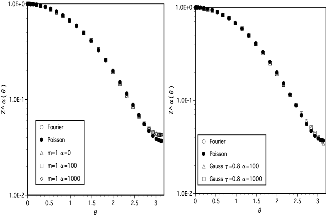
Figure 3: ${\cal Z}^{(\alpha)}(\theta)$ for the data without flattening. Here, $V=12$. The default model $m(\theta)$ is chosen to be the constant 1.0 and the Gaussian function with $\gamma=0.8$.

The number of degrees of freedom in $\theta$ space, $N_{\theta}$, is larger than that of the topological charge, $N_{q}$. The number $N_{q}$ was chosen so as to satisfy $P(Q)\geq 10^{-30}$ in the non-flattening case and $P(Q)\geq 10^{-11}$ in the flattening case, and it varies from 3 to 8, depending on $V$. The covariance matrix appears in Eq. (15):

$$C_{Q,Q^{\prime}}=\frac{1}{N_{d}(N_{d}-1)}\sum_{l=1}^{N_{d}}(P^{(l)}(Q)-{\bar{P}}(Q))(P^{(l)}(Q^{\prime})-{\bar{P}}(Q^{\prime})),$$ (37)

where $P^{(l)}(Q)$ denotes the $l$-th data of the topological charge distribution and ${\bar{P}}(Q)$ is the average Eq. (16). The inverse covariance matrix is calculated with such precision that the product of the covariance matrix and its inverse has off-diagonal elements that are at most ${\cal O}(10^{-27})$.

The number of the other degrees of freedom, $N_{\theta}$, was varied from 10 to 100, and it was found that the results are stable for $25\hskip 3.00003pt\raisebox{1.72218pt}{$<$}\raisebox{-3.01385pt}{$\sim$}\hskip 3.00003ptN_{\theta}$. In the following results, $N_{\theta}$ is set to be 28. Note that in order to reproduce ${\cal Z}(\theta)$, which ranges over many orders, the analysis must be performed with quadruple precision.

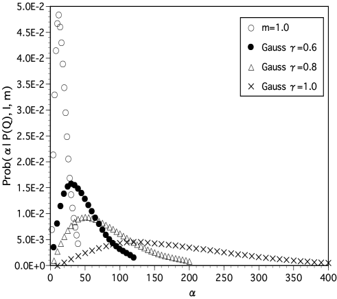
Figure 4: ${\rm prob}(\alpha|P(Q),I,m)$ for the data without flattening. Here, $V=12$. The default model is chosen to be the constant $m(\theta)=1.0$ and the Gaussian function with $\gamma=0.6$, 0.8 and 1.0.

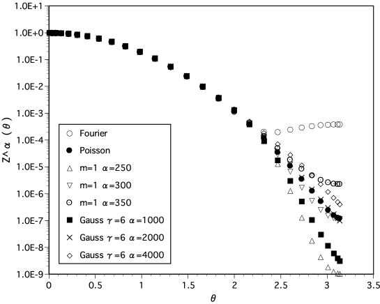
Figure 5: ${\cal Z}^{(\alpha)}(\theta)$ for the data with flattening. The default model $m(\theta)$ is chosen to be the constant 1.0 and the Gaussian function with $\gamma=6$. Comparing with the result of the Fourier transform (circles), the result of the MEM for certain values of $\alpha$ ($\alpha\approx 300$ for $m(\theta)=1.0$ and $\alpha\approx 2000$ for the Gaussian) approximately reproduces that of the exact partition function Eq. (4) (filled circles).

4.1 MEM analysis of the data without flattening

Before discussing to what extent the flattening behavior of the free energy is remedied, we discuss the case without flattening. It is a non-trivial question whether the MEM is effective in the application considered here.

The data for $V\leq 20$ were used in the analysis. For such data, no flattening behavior is observed (see Fig. 2). For the present, we concentrate on the data for $V=12$. For this value of $V$, two types of default models were employed, the constant default model, $m(\theta)=1.0$, and the Gaussian one with $\gamma=0.4-1.0$.

The maximal image ${\cal Z}^{(\alpha)}(\theta)$ of ${\cal Z}(\theta)$ for a given $\alpha$ was calculated using Eq. (22). Figure 3 displays ${\cal Z}^{(\alpha)}(\theta)$ calculated in this way for various $\alpha$ ($0\leq\alpha\leq 1000$) in the cases that $m(\theta)$ is the constant 1.0 and the Gaussian function with $\gamma=0.8$. It is found that there is almost no discernible $\alpha$ dependence of ${\cal Z}^{(\alpha)}(\theta)$ and that the images approximately agree with the result of the Fourier transform, and thus with the exact partition function ${\cal Z}_{{\rm pois}}(\theta)$.

In order to determine which ${\cal Z}^{(\alpha)}(\theta)$ is the most probable, we calculated the posterior probability ${\rm prob}(\alpha|P(Q),I,m)$ in Eq. (31). The data for ${\rm prob}(\alpha|P(Q),I,m)$ were fitted by smooth functions and normalized such that Eq. (33) holds. The results are plotted in Fig. 4. For both cases, ${\rm prob}(\alpha|P(Q),I,m)$ has a peak at a small value of $\alpha$; for $m(\theta)=1.0$, the peak is located at $\alpha\simeq 12.0$, while in the Gaussian case it is located at $\alpha\simeq 30.0$ $(\gamma=0.6)$, $\alpha\simeq 50.0$ $(\gamma=0.8)$ and $\alpha\simeq 120.0$ $(\gamma=1.0)$. Because the functions ${\cal Z}^{(\alpha)}(\theta)$ do not depend on $\alpha$ in the region around the peak, the integrals we must evaluate to obtain the averaged image ${\hat{\cal Z}}(\theta)$ in Eq. (31) are trivially simple, and the functions ${\hat{\cal Z}}(\theta)$ are approximately in agreement with the exact one.

For $V=8$ and 20, similar analyses were carried out. We find that the characteristics of ${\cal Z}^{(\alpha)}(\theta)$ and ${\rm prob}(\alpha|P(Q),I,m)$ stated above, namely, that ${\cal Z}^{(\alpha)}(\theta)$ is almost independent of $\alpha$ for not so large values ($\alpha\hskip 3.00003pt\raisebox{1.72218pt}{$<$}\raisebox{-3.01385pt}{$\sim$}\hskip 3.00003pt1000$) and ${\rm prob}(\alpha|P(Q),I,m)$ has a peak at a small value of $\alpha$, are also observed for $V=8$ and 20. Therefore, we obtain the same results for ${\hat{\cal Z}}(\theta)$. More generally, in the non-flattening case, where the Fourier transform works well, the fact that the image obtained using the MEM is consistent with the result of the Fourier transform can be understood by carefully considering the equations used in the SVD. This is investigated analytically in Appendix D.

The detailed procedure for estimating the error $\delta{\hat{\cal Z}}(\theta)$ is discussed in the next subsection, and its results are given at the end.

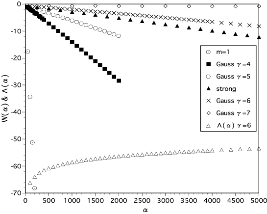
Figure 6: $W({\cal Z}^{(\alpha)})$ for various $m(\theta)$ and for $V=50$. $W({\cal Z}^{(\alpha)})$ is plotted for $m_{\rm strg}(\theta)$ and for the Gaussian default models with $\gamma=4,5,6$ and 7. $\Lambda(\alpha)$ appearing in Eq. (31) is also plotted on the same scale. Because $\Lambda(\alpha)$ does not depend strongly on $m(\theta)$, $\Lambda(\alpha)$ for the Gaussian default model with $\gamma=6$ is displayed as a reference.

4.2 MEM analysis of the data with flattening

Let us now turn to the case with flattening. Unlike the case without flattening, in this case the images of ${\cal Z}(\theta)$ display behavior that differs greatly from those of the Fourier transform. We fix the volume to $V=50$ for the time being. Figure 5 displays ${\cal Z}^{(\alpha)}(\theta)$ calculated with $m(\theta)$ given by the constant 1.0 and the Gaussian form with $\gamma=6$, which are images determined by maximizing Eq. (21) for each $\alpha$. For each of the defaults, the maximal images are free from flattening, and at least for a certain value of $\alpha$, there exists a ${\cal Z}^{(\alpha)}(\theta)$ which is in reasonable agreement with the exact one, ${\cal Z}_{\rm pois}(\theta)$. This also holds in the case that $m(\theta)$ is Gaussian with $\gamma=4,5$ and 7, although the value of $\alpha$ for which we find the best agreement with ${\cal Z}_{\rm pois}(\theta)$ depends on $\gamma$. In the case of $m_{\rm strg}(\theta)$, however, we find no agreement, even when $\alpha$ is varied from ${\cal O}$(1) to ${\cal O}(10^{6})$.

The posterior probability ${\rm prob}(\alpha|P(Q),I,m)$ was calculated with Eq. (51) appearing in Eq. (31). Figure 6 displays the behavior of $W({\cal Z}^{(\alpha)})$ and $\Lambda(\alpha)$ for various $m(\theta)$. We find that as $\alpha$ increases, $W({\cal Z}^{(\alpha)})$ decreases almost linearly, depending strongly on $m(\theta)$, while $\Lambda(\alpha)$ increases with rather weak $\alpha$ dependence. The sum of $W({\cal Z}^{(\alpha)})$ and $\Lambda(\alpha)$ gives ${\rm prob}(\alpha|P(Q),I,m)$, and the balance between the two determines the location of the peak of ${\rm prob}(\alpha|P(Q),I,m)$, if it exists. This is shown in Fig. 7.

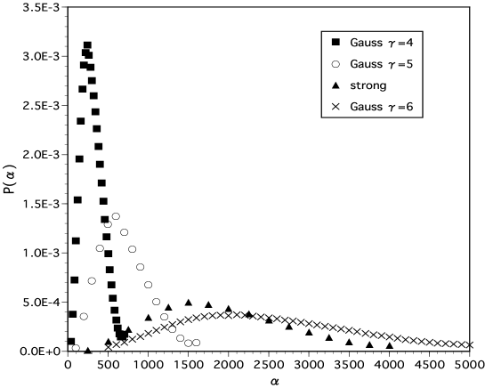
Figure 7: ${\rm prob}(\alpha|P(Q),I,m)$ for various $m(\theta)$. $V$ is fixed to 50.

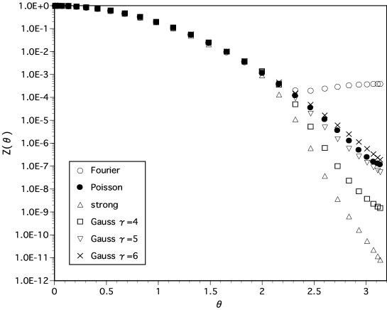
Figure 8: Averaged partition function $\hat{{\cal Z}}(\theta)$ for various $m(\theta)$. The volume is fixed to 50. The result of the Fourier transform is also included. Those for the Gaussian default models with $\gamma=5$ and 6 agree reasonably with the exact result, ${\cal Z}_{\rm pois}(\theta)$. The result for $m_{\rm strg}(\theta)$ shows a large deviation from ${\cal Z}_{\rm pois}(\theta)$.

The averaged image $\hat{{\cal Z}}(\theta)$ was calculated using Eq. (31). Integrating over $\alpha$, the data for ${\rm prob}(\alpha|P(Q),I,m)$ were fitted by a smooth function. Then, the fitting function was normalized. Figure 8 displays $\hat{{\cal Z}}(\theta)$ for various $m(\theta)$. In the case of a Gaussian $m(\theta)$, the parameter $\gamma$ is varied from 4 to 8. We find reasonably good agreement between the function ${\hat{\cal Z}}(\theta)$ for $\gamma=5$ and 6. This is due to the fact that for these cases, the best value of $\alpha$ for ${\cal Z}^{(\alpha)}(\theta)$ is approximately equal to the location of the peak of ${\rm prob}(\alpha|P(Q),I,m)$; for $\gamma=6$ the two values are nearly equal($\approx$ 2000), while for $\gamma=5$ they differ slightly ($\approx$ 1000 for the former and $\approx$ 650 for the latter). In other words, these images could occur with high probability.

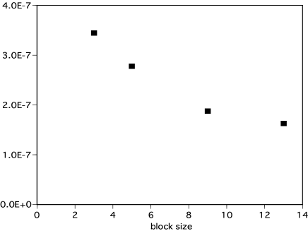
Figure 9: Errors estimated at $\theta=3.07$ by varying the block size for $\gamma=5.5$ and $V=50$. (See the text for details.)

Table 1: $\hat{{\cal Z}}(\theta)$ and error at $\theta=3.07$ for the various default models depicted in Fig. 8. The exact value, ${\cal Z}_{\rm pois}(3.07)$, is $1.554\times 10^{-7}$.

$m(\theta)$	$\hat{{\cal Z}}(3.07)$		$\delta\hat{{\cal Z}}(3.07)$
strong	2.	33$\times 10^{-11}$	3.	5$\times 10^{-8}$
Gauss $\gamma=4$	2.	29$\times 10^{-9}$	7.	4$\times 10^{-8}$
Gauss $\gamma=5$	8.	99$\times 10^{-8}$	1.	9$\times 10^{-7}$
Gauss $\gamma=6$	3.	38$\times 10^{-7}$	1.	7$\times 10^{-7}$

In the $m(\theta)=1.0$ case, although the best image is in good agreement with ${\cal Z}_{\rm pois}(\theta)$ for $\alpha=300$, as shown in Fig. 5, the peak of ${\rm prob}(\alpha|P(Q),I)$ is located in the region where $\alpha<40.0$. This large difference in $\alpha$ leads to a large deviation of $\hat{{\cal Z}}(\theta)$ from the correct one, ${\cal Z}_{\rm pois}(\theta)$. Similarly, for $m_{\rm strg}(\theta)$, the image ${\cal Z}^{(\alpha)}(\theta)$ in agreement with ${\cal Z}_{\rm pois}(\theta)$ occurs with a very low probability, and consequently $\hat{{\cal Z}}(\theta)$ deviates greatly from ${\cal Z}_{\rm pois}(\theta)$. This is obvious, because ${\cal Z}^{(\alpha)}(\theta)$ never agrees with ${\cal Z}_{\rm pois}(\theta)$ for $\alpha={\cal O}(1)$ to ${\cal O}(10^{6})$. (Note that the errors are not included in the figure.)

One of the advantages of the MEM analysis is that it allows estimation of the error according to the probability that the images are realized. In fact, the obtained images are meaningless unless their errors are evaluated. We use the formula Eq. (36) for the error estimates. The error $\delta\hat{{\cal Z}}(\theta_{n})$ of $\hat{{\cal Z}}(\theta_{n})$ is estimated by integrating $\theta$ in Eq. (36) over the range $\Theta=\theta_{n-b/2}$ and $\theta_{n+b/2}$, where $\theta_{m}$ is the abscissa in the Gauss-Legendre $N$-point ($N$=100) quadrature formula for the range $0\leq\theta\leq\pi$. Figure 9 displays typical behavior of the error as a function of the block size at $\theta=3.07$ for Gaussian $m(\theta)$ with $\gamma=5.5$, where the block size is defined by $b+1$.

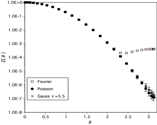
Figure 10: $\hat{{\cal Z}}(\theta)$ (crosses) with the error bars for the Gaussian default model with $\gamma=5.5$. Here, $V=50$. Compared to the result of the Fourier transform (circles), a remarkable improvement is clearly seen.

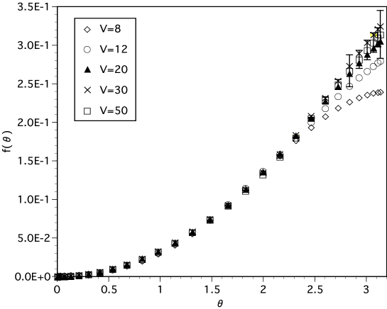
Figure 11: Free energy density $f(\theta)$ calculated from $\hat{{\cal Z}}(\theta)$ for various volumes. (See Fig. 2 for a comparison.)

Table 2: $\hat{{\cal Z}}(\theta)$ at $\theta=2.30$ and $\theta=3.07$ for various volumes $V$. The default model is chosen to be the Gaussian form with $\gamma$. The exact values ${\cal Z}_{\rm pois}(\theta)$ are also listed.

$V$	$\gamma$ (Gaussian default)	${\cal Z}_{\rm pois}(2.30)$		$\hat{{\cal Z}}(2.30)$		${\cal Z}_{\rm pois}(3.07)$		$\hat{{\cal Z}}(3.07)$
8	0.1	2.	493$\times 10^{-1}$	2.	424(3)$\times 10^{-1}$	1.	407$\times 10^{-1}$	1.	48491(6)$\times 10^{-1}$
12	0.8	1.	155$\times 10^{-2}$	1.	145(3)$\times 10^{-2}$	3.	752$\times 10^{-2}$	3.	762(1)   $\times 10^{-2}$
20	1.6	2.	676$\times 10^{-2}$	2.	583(2)$\times 10^{-2}$	2.	697$\times 10^{-3}$	2.	946(6)   $\times 10^{-3}$
30	3.4	4.	372$\times 10^{-3}$	4.	12(2)$\;\;\times 10^{-3}$	1.	023$\times 10^{-4}$	8.	3(3)      $\times 10^{-4}$
50	5.5	1.	169$\times 10^{-4}$	1.	20(4)$\;\;\times 10^{-4}$	1.	554$\times 10^{-7}$	2.	5(1.6)  $\;\;\times 10^{-7}$

In order to show how large the errors of $\hat{{\cal Z}}(\theta)$ in Fig. 8 are in the region near $\theta=\pi$, Table 1 lists the values of $\hat{{\cal Z}}(\theta)$ and their errors at $\theta=3.07$. Together with the results displayed in Fig. 8, we find that the more $\hat{{\cal Z}}(\theta)$ deviates from the exact one, the larger the magnitude of the relative error becomes.

Among the default models we have investigated, it turns out that the errors for the Gaussian form with $\gamma=5.5$ are the smallest. Figure 10 plots the partition function with the estimated errors for the Gaussian default model with $\gamma=5.5$. The result is consistent with ${\cal Z}_{\rm pois}(\theta)$ and does not exhibit flattening. For the other default models, $m(\theta)=1.0$ and $m_{\rm strg}(\theta)$, it is found that the errors are too large to obtain reasonable images ${\hat{\cal Z}}(\theta)$.

We applied the same procedure to the data for other volumes. Table 2 gives $\hat{{\cal Z}}(\theta)$ and $\delta\hat{{\cal Z}}(\theta)$ at $\theta=2.30$ and 3.07 for various volumes and default models. Each of the two values of $\theta$ was chosen as a reference, where the latter is close to $\pi$ and the former is near $\theta_{\rm f}$. The default models listed in Table 2 give almost minimal errors among the defaults we have investigated for each volume. These were used to calculate the free energy density plotted in Fig. 11. We find by comparing Fig. 2 that the flattening behavior is no longer observed.

5 Summary

We have considered lattice field theory with a $\theta$ term. When studied numerically, this theory suffers from the complex Boltzmann weight problem, or the sign problem. As an attempt at an approach that differs from the conventional procedure, which employs the numerical Fourier transform of $P(Q)$, we have applied the MEM in order to reconstruct the partition function ${\cal Z}(\theta)$. In the MEM analysis, the image of ${\cal Z}(\theta)$ is calculated probabilistically, and the error is estimated as the uncertainty of the image. We have employed the Gaussian $P(Q)$ as a test, because its Fourier transform can be computed analytically. We found that for the data without flattening, the results of the MEM analysis are consistent with those of the Fourier transform, while for those with flattening, the MEM reproduces reasonable images that exhibit no flattening by reducing the error contained in the data of $P(Q)$ ($\delta\approx 1/400$).

Comments are in order.

1. During the analysis, the condition ${\cal Z}(\theta)>0$ in Eq. (20) was imposed as prior information $I$. This plays an important role in searching for the maximal image in the case with flattening. This condition could yield results that differ from those found in the Fourier method, where ${\cal Z}(\theta)$ could become negative due to large error.

2. It is important what default model is chosen for the analysis. A criterion for this choice is the magnitude of the errors of the averaged image, which are determined according to the probability. We have investigated various default models and found that $\gamma=3.4$ for $V=30$ and $\gamma=5.5$ for $V=50$ are the best among those which we have investigated in the flattening case. The purpose of the present paper is to check the feasibility of the application of the MEM to the case with the $\theta$ term, and therefore we did not consider a large number of Gaussian defaults with different values of $\gamma$. There might be some better default models than those we have investigated here.

3. The final image ${\cal Z}(\theta)$ depends on $\delta$, which controls the magnitude of the error of the mock data $P(Q)$. The parameter $\delta$ directly affects the covariance matrix and indirectly influences the error $\delta\hat{{\cal Z}}(\theta)$ of the image, which is the uncertainty of the image. Although we employed the least uncertainty as a criterion, it is still unclear to what extent the obtained best image is close to the true one; i.e., there is a systematic error in $\hat{{\cal Z}}(\theta)$, not reflected in $\delta\hat{{\cal Z}}(\theta)$. This is related to the freedom that we have in choosing the default model. Various default models may be allowed within the uncertainty related to $\delta$. To check this point we may as well use the mock data that causes true flattening behavior of the free energy and study the interference of such an effect with the data used in the present study. This will be studied in a forthcoming paper. Furthermore, some objective analysis of the parameter inference is needed with regard to the regularization of the unfolding problem [22].

4. As the volume increases, the flattening problem becomes more severe, and higher precision of the computations becomes necessary. This is because a more precise calculation is required to obtain the inverse of the covariance matrix of $P(Q)$ as the volume increases. In the case $V=8$, for example, the Newton method with double precision is sufficient. For $V=50$, however, we need quadruple precision.

5. Because the flattening behavior is inherent in the Fourier procedure, no matter what model one treats, we have used the Gaussian $P(Q)$ as a first attempt. The next step is to apply the MEM to more realistic models, such as the CP^N-1 model and QCD, and to investigate its feasibility for them. The MEM analysis might also be applicable to some other models with the sign problem. It may be worthwhile to study whether it is effective for treating theories such as lattice field theory with a finite density.

Appendix A SVD and the Newton Method

In order to obtain the maximal image of ${\cal Z}(\theta)$ for fixed $\alpha$, we must solve the following equation [see Eq. (22)]:

$$-\alpha\log\frac{{\cal Z}_{n}}{m_{n}}=\sum_{ij}K_{jn}C_{ij}^{-1}\delta P_{j}.$$ (38)

For later convenience, we introduce a new parameter $a_{n}$ defined by

$$a_{n}\equiv\log\frac{{\cal Z}_{n}}{m_{n}}.$$ (39)

We regard ${\cal Z}_{n}$ and $\bar{P}_{j}$ as $N_{\theta}$- and $N_{q}$-dimensional vectors, respectively ($n=1,2,\cdots,N_{\theta}\;\mbox{and}\;j=1,2,\cdots,N_{q}$). In our case, $N_{\theta}\sim{\cal O}(10^{1})-{\cal O}(10^{2})$ and $N_{q}\sim{\cal O}(10^{0})$. Therefore, it is non-trivial to find ${\cal Z}^{(\alpha)}_{n}$ satisfying Eq. (22). This task is made considerably simpler by employing the SVD. The transpose of $K$, $K^{t}$, is decomposed as

$$(K^{t})_{nj}=(U\Xi V^{t})_{nj},$$ (40)

where $U$ is an $N_{\theta}\times N_{q}$ matrix satisfying $U^{t}U=1$, $V$ is an $N_{q}\times N_{q}$ orthogonal matrix, and $\Xi$ is an $N_{q}\times N_{q}$ diagonal matrix, $(\Xi)_{ij}=\xi_{i}\delta_{ij}$. The eigenvalues $\xi_{i}$, which are positive semi-definite, are called the ‘singular values’ of $K^{t}$. They could be arranged by appropriate permutations such that $\xi_{1}\geq\xi_{2}\geq\cdots\geq\xi_{N_{s}}>\xi_{N_{s+1}}=\cdots=\xi_{N_{q}}=0$, where

$$N_{s}={\rm rank}(K^{t})\leq N_{q}.$$ (41)

Following Bryan[13], the first $N_{s}$ column vectors of $U=({\bm{u}}_{1},{\bm{u}}_{2},\cdots,{\bm{u}}_{N_{q}})$ construct a basis in ‘singular space’, which is a subspace of the $N_{\theta}$-dimensional space whose basis is $\{{\bm{u}}_{1},{\bm{u}}_{2},\cdots,{\bm{u}}_{N_{s}}\}$, with ${\bm{u}}_{i}=(u_{1i}.u_{2i},\cdots,u_{N_{\theta}i})^{t}$. One can then place the vector ${\bm{a}}$ in singular space

$${\bm{a}}=\sum_{i=1}^{N_{s}}\lambda_{i}{\bm{u}}_{i}.$$ (42)

Substituting Eqs. (40) and (42) into Eq. (38), we find

$$-\alpha\sum_{i}\lambda_{i}U_{ni}=\sum_{i,j}(U\Xi V^{t})_{ni}C_{ij}^{-1}\delta P_{j}.$$ (43)

Use of $U^{t}U=1$ then yields

$$-\alpha\lambda_{i}=\sum_{j,l}(\Xi V^{t})_{ij}C_{jl}^{-1}\delta P_{l}.$$ (44)

To solve $\lambda_{i}$, the Newton method is employed. For each iteration, an increment $\delta{\bf\lambda}$ is given by

$$\sum_{k}\Biggl{[}-\alpha\delta_{ik}-\sum_{j,l,n}(\Xi V^{t})_{ij}C_{jl}^{-1}K_{ln}{\cal Z}_{n}U_{nk}\Biggr{]}\delta\lambda_{k}=\alpha\lambda_{i}+\sum_{j,l}(\Xi V^{t})_{ij}C_{jl}^{-1}\delta P_{l},$$ (45)

or in the matrix notation,

$$-X\delta{\bf\lambda}=\alpha\lambda+Y\delta P,$$ (46)

where $\lambda$ and $\delta P$ are $N_{q}$-dimensional vectors, and $X$ and $Y$ are $N_{s}\times N_{s}$ and $N_{s}\times N_{q}$ matrices, respectively:

$$X\equiv\alpha{\bf 1}+\Xi V^{t}C^{-1}K{\cal Z}U,\qquad Y\equiv\Xi V^{t}C^{-1}.$$ (47)

We then need to calculate the inverse matrix of $X$ to obtain $\delta{\bf\lambda}$. Note that $N_{s}=N_{q}$ holds for all the cases we have considered in the present paper.

Appendix B Derivation of Eqs. (31) and (36)

1. Equation (31) is derived as follows.

   The probability ${\rm prob}({\cal Z}_{n}|P(Q),I,m)$ can be rewritten by use of the law of the total probability ${\rm prob}(A)=\int dB\;{\rm prob}(A,B)$ as follows:

   $${\rm prob}({\cal Z}_{n}|P(Q),I,m) = \int d\alpha~{}{\rm prob}({\cal Z}_{n},\alpha|P(Q),I,m)$$

   $$= \int d\alpha~{}{\rm prob}({\cal Z}_{n}|\alpha,P(Q),I,m){\rm prob}(\alpha|P(Q),I,m).$$

   In the second line, the definition of the conditional probability was used.

   Substituting Eq. (LABEL:eqn:totalprobability) into Eq. (29), we obtain

   $${\hat{\cal Z}}_{n} = \int[d{\cal Z}]{\cal Z}_{n}\int d\alpha~{}{\rm prob}({\cal Z}_{n}|\alpha,P(Q),I,m){\rm prob}(\alpha|P(Q),I,m)$$ (49)

   $$= \int d\alpha~{}{\rm prob}(\alpha|P(Q),I,m)\int[d{\cal Z}]{\cal Z}_{n}~{}{\rm prob}({\cal Z}_{n}|\alpha,P(Q),I,m)$$

   $$\simeq \int d\alpha~{}{\rm prob}(\alpha|P(Q),I,m){\cal Z}^{(\alpha)}_{n},$$

   where we have assumed that the probability ${\rm prob}({\cal Z}_{n}|\alpha,P(Q),I,m)$ has a sharp peak around ${\cal Z}^{(\alpha)}_{n}$. Utilizing Bayes’ theorem, the law of the total probability, and the definition of the conditional probability, the probability ${\rm prob}(\alpha|P(Q),I,m)$ can be rewritten as

   $${\rm prob}(\alpha|P(Q),I,m) = \frac{{\rm prob}(P(Q)|\alpha,I,m){\rm prob}(\alpha|I,m)}{{\rm prob}(P(Q)|I,m)}$$ (50)

   $$= \frac{{\rm prob}(\alpha|I,m)}{{\rm prob}(P(Q)|I,m)}\int[d{\cal Z}]~{}{\rm prob}(P(Q),{\cal Z}_{n}|\alpha,I,m)$$

   $$= \frac{{\rm prob}(\alpha|I,m)}{{\rm prob}(P(Q)|I,m)}\int[d{\cal Z}]~{}{\rm prob}(P(Q)|{\cal Z}_{n},\alpha,I,m)$$

   $$\;\;\;\;\;\;\;\;\;\;\;\;\;\;\;\;\;\;\;\;\;\;\;\;\;\;\;\;\;\;\;\;\times{\rm prob}({\cal Z}_{n}|\alpha,I,m)$$

   $$\propto {\rm prob}(\alpha|I,m)\int[d{\cal Z}]\frac{e^{W({\cal Z})}}{X_{L}X_{S}(\alpha)},$$

   where Eq. (19) has been used and irrelevant factors, such as ${\rm prob}(P(Q)|I,m)$, have been ignored.

   Expanding $W({\cal Z})$ around $\{{\cal Z}^{(\alpha)}\}$ up to second order, we can perform the Gaussian integration over configurations of $\{{\cal Z}\}$:

   $${\rm prob}(\alpha|P(Q),I,m)$$ (51)

   $$\propto {\rm prob}(\alpha|I,m)\int[d{\cal Z}]\frac{1}{X_{L}X_{S}(\alpha)}\exp\biggl{\{}W({\cal Z}^{(\alpha)})+\frac{1}{2}\sum_{n,n^{\prime}}\delta{\cal Z}_{n}\frac{\partial^{2}W}{\partial{\cal Z}_{n}\partial{\cal Z}_{n^{\prime}}}\delta{\cal Z}_{n^{\prime}}\biggr{\}}$$

   $$\propto {\rm prob}(\alpha|I,m)\exp\biggl{\{}\frac{1}{2}\sum_{k}\log\frac{\alpha}{\alpha+\lambda_{k}}+W({\cal Z}^{(\alpha)})\biggr{\}}$$

   $$\equiv {\rm prob}(\alpha|I,m)\exp\biggl{\{}\Lambda(\alpha)+W({\cal Z}^{(\alpha)})\biggr{\}},$$

   where $\delta{\cal Z}_{n}\equiv{\cal Z}_{n}-{\cal Z}_{n}^{(\alpha)}$. Irrelevant constants have been ignored here, as before. The values $\lambda_{k}$ are eigenvalues of the real symmetric matrix in $\theta$ space defined in Eq. (32). The prior probability ${\rm prob}(\alpha|I,m)$ is conventionally chosen to be either the Laplace rule [${\rm prob}(\alpha|I,m)=$const.] or the Jeffrey rule [${\rm prob}(\alpha|I,m)=1/\alpha$]. Because the integral in Eq. (49) is insensitive to the choice of ${\rm prob}(\alpha|I,m)$ as long as ${\rm prob}(\alpha|P(Q),I,m)$ has a sharp peak, we employ the Laplace rule for simplicity. [17, 13]

   Substituting Eq. (51) into Eq. (49), we can obtain the equation for ${\hat{\cal Z}}_{n}$,

   $${\hat{\cal Z}}_{n}=\frac{1}{X_{W}}\int d\alpha{\cal Z}^{(\alpha)}_{n}\exp\biggl{\{}\frac{1}{2}\sum_{k}\log\frac{\alpha}{\alpha+\lambda_{k}}+W({\cal Z}^{(\alpha)})\biggr{\}}.$$ (52)

2. Equation (36) is derived as follows.

   The uncertainty of the final output image ${\hat{\cal Z}}_{n}$ is calculated as follows: [16, 17]

   $$\langle(\delta{\hat{\cal Z}}_{n})^{2}\rangle\equiv\int d\alpha\langle(\delta{\cal Z}^{(\alpha)}_{n})^{2}\rangle{\rm prob}(\alpha|P(Q),I,m),$$ (53)

   where

   $$\langle(\delta{\cal Z}_{m}^{(\alpha)})^{2}\rangle\equiv\frac{\int[d{\cal Z}]\int_{\Theta}d\theta_{n}d\theta_{n^{\prime}}\delta{\cal Z}_{n}\delta{\cal Z}_{n^{\prime}}{\rm prob}({\cal Z}_{m}|P(Q),I,m,\alpha)}{\int[d{\cal Z}]\int_{\Theta}d\theta_{n}d\theta_{n^{\prime}}{\rm prob}({\cal Z}_{m}|P(Q),I,m,\alpha)}.$$ (54)

   Using $\int[d{\cal Z}]~{}{\rm prob}({\cal Z}_{m}|P(Q),I,m,\alpha)\equiv 1$ and inserting Eq. (19), we obtain

   $$\langle(\delta{\cal Z}_{m}^{(\alpha)})^{2}\rangle=\frac{1}{\int_{\Theta}d\theta_{n}d\theta_{n^{\prime}}}\int_{\Theta}d\theta_{n}d\theta_{n^{\prime}}\int[d{\cal Z}]\delta{\cal Z}_{n}\delta{\cal Z}_{n^{\prime}}\frac{e^{W({\cal Z})}}{X_{L}X_{S}(\alpha)}.$$ (55)

   When $e^{W({\cal Z})}$ is expanded around $\{{\cal Z}^{(\alpha)}\}$ up to second order, and the integral over ${\cal Z}_{n}$ is performed, Eq. (36) is derived as

   $$\langle(\delta{\cal Z}_{m}^{(\alpha)})^{2}\rangle = \frac{1}{\int_{\Theta}d\theta_{n}d\theta_{n^{\prime}}}\int_{\Theta}d\theta_{n}d\theta_{n^{\prime}}\int[d{\cal Z}]\delta{\cal Z}_{n}\delta{\cal Z}_{n^{\prime}}\frac{1}{X_{L}X_{S}(\alpha)}$$ (56)

   $$\;\;\;\;\;\;\;\;\;\;\;\;\;\;\;\;\;\times\exp\biggl{\{}W({\cal Z}^{(\alpha)})+\frac{1}{2}\sum_{n,n^{\prime}}\delta{\cal Z}_{n}\frac{\partial^{2}W}{\partial{\cal Z}_{n}\partial{\cal Z}_{n^{\prime}}}\delta{\cal Z}_{n^{\prime}}\biggr{\}}$$

   $$\simeq -\frac{1}{\int_{\Theta}d\theta_{n}d\theta_{n^{\prime}}}\int_{\Theta}d\theta_{n}d\theta_{n^{\prime}}\Bigl{(}\frac{\partial^{2}W}{\partial{\cal Z}_{n}\partial{\cal Z}_{n^{\prime}}}\Bigm{|}_{{\cal Z}={\cal Z}^{(\alpha)}}\Bigr{)}^{-1}.$$

Appendix C Uniqueness of the Maximum of $W$

Following Asakawa et. al. [17], let us check that a unique maximum of $W$ exists for $\alpha\neq 0~{}(>0)$. In our case, the kernel is given by that of the Fourier transform. The curvature of $W$ is given by

$$\frac{\partial^{2}W}{\partial{\cal Z}_{m}\partial{\cal Z}_{n}}=-\alpha\delta_{mn}\frac{1}{{\cal Z}_{n}}-\sum_{ij}K_{im}C^{-1}_{ij}K_{jn}.$$ (57)

Introducing any $N_{\theta}$-dimensional real vector ${\bm{y}}(\neq 0)$, let us calculate

$$\sum_{mn}y_{m}\frac{\partial^{2}W}{\partial{\cal Z}_{m}\partial{\cal Z}_{n}}y_{n}=\sum_{mn}y_{m}\Biggl{[}-\alpha\delta_{mn}\frac{1}{{\cal Z}_{n}}-\sum_{ij}K_{im}C^{-1}_{ij}K_{jn}\Biggr{]}y_{n}.$$ (58)

1. $\alpha=0$ case

   When $\alpha=0$, Eq. (58) becomes

   $$\sum_{mn}y_{m}\frac{\partial^{2}W}{\partial{\cal Z}_{m}\partial{\cal Z}_{n}}y_{n}=-\sum_{mn}y_{m}\sum_{ij}K_{im}C^{-1}_{ij}K_{jn}y_{n}.$$ (59)

   Because the covariance matrix $C$ is symmetric, $C$ is diagonalized by an $N_{q}\times N_{q}$ orthogonal matrix $R$ as

   $$R^{t}CR=\bar{\sigma}^{2}.$$

   Also, defining the $N_{q}\times N_{\theta}$ matrix

   $$\tilde{K}\equiv R^{t}K$$

   and the $N_{q}$-dimensional real vector

   $$\tilde{\bm{y}}\equiv\tilde{K}{\bm{y}},$$ (60)

   Eq. (59) becomes

   $$\sum_{mn}y_{m}\frac{\partial^{2}W}{\partial{\cal Z}_{m}\partial{\cal Z}_{n}}y_{n}=-\sum_{i}\frac{\tilde{y}^{2}_{i}}{\bar{\sigma}^{2}_{i}}\leq 0.$$ (61)

   This could vanish only for $\tilde{\bm{y}}=0$, and this is realized for non-trivial vectors ${\bm{y}}$, because Eq. (60) asserts that the dimension of the solution vector space is

   $$N_{\theta}-{\rm rank}\tilde{K}\geq N_{\theta}-N_{q}>0.$$

   In the $\alpha=0$ case, therefore, there are multiple maxima of $W$.

2. $\alpha\neq 0$ case

   For $\alpha\neq 0$, Eq. (58) becomes

   $$\sum_{mn}y_{m}\frac{\partial^{2}W}{\partial{\cal Z}_{m}\partial{\cal Z}_{n}}y_{n}=-\alpha\sum_{n}\frac{y_{n}^{2}}{{\cal Z}_{n}}-\sum_{i}\frac{\tilde{y}^{2}_{i}}{\bar{\sigma}^{2}_{i}}.$$ (62)

   Because ${\cal Z}_{n}>0$, the curvature of $W$ becomes negative definite:

   $$\sum_{nm}y_{m}\frac{\partial^{2}W}{\partial{\cal Z}_{m}\partial{\cal Z}_{n}}y_{n}<0.$$

   Therefore, the entropy term is essential to the uniqueness of the maximum.

Appendix D Comparison with the Fourier Method

In the case of no flattening, we show that the analysis in the Newton method leads to the same result as that obtained using the Fourier method. This holds for $\alpha=0$ and $\alpha\neq 0$ (but only small $\alpha>0$). Note that in the Fourier method,

$${\bar{P}}=K{\cal Z}$$ (63)

is successfully inverted in the case without flattening. This is because $P(Q)$ is a rapidly decreasing function, and ${\cal Z}(\theta)$, which is given by the Fourier transform, is smooth enough that the contribution from higher $Q$ can be ignored.

1. $\alpha=0$ case

   Let us first consider the $\alpha=0$ case. For $\alpha=0$, Eq. (46) reduces to

   $$-X_{0}\delta{\bf\lambda}=Y\delta P,$$ (64)

   where

   $$X_{0}\equiv\Xi V^{t}C^{-1}KZU.$$ (65)

   When $X_{0}$ is regular, the increment $\delta\lambda$ becomes

   $$\delta\lambda=-X_{0}^{-1}Y\delta P.$$ (66)

   When the integrations converge, i.e., when $\delta\lambda=0$, in the Newton method, we find

   $$X_{0}^{-1}Y\delta P=0.$$ (67)

   Because the $N_{q}\times N_{q}$ matrix $X_{0}^{-1}Y$ is regular (this can be checked numerically),

   $$\delta P=K{\cal Z}-\bar{P}=0$$ (68)

   is a unique solution.

   Equation (68) gives $N_{q}$ equations:

   $$\sum_{n=1}^{N_{\theta}}K_{in}m_{n}\exp(\sum_{j=1}^{N_{q}}U_{nj}\lambda_{j})=\bar{P}_{i}\qquad(i=1,\dots,N_{q}).$$ (69)

   Thus, one obtains a unique solution for $\lambda_{i}(i=1,\dots,N_{q})$ for a given default $m_{n}$. This turns out to give a ${\cal Z}_{n}$ that is equivalent to that found in the Fourier method.

2. $\alpha\neq 0$ case (small $\alpha$)

   When $\alpha\neq 0$, we use Eq. (46) in the Newton method. For small $\alpha$, this is approximated by

   $$X\delta\lambda=-Y\delta P.$$ (70)

   By using the regularity of $X$, $\delta\lambda$ is given by

   $$\delta\lambda=-X^{-1}Y\delta P.$$ (71)

   When the integration converges, $\delta\lambda=0$, the regularity of $X^{-1}Y$ implies

   $$\delta P=0,$$ (72)

   which is the same as Eq. (68). Therefore we obtain a unique solution in this case too.

We thus find that for $\alpha=0$ and/or for small values of $\alpha$, the Newton method leads to the same result ${\cal Z}^{(\alpha)}_{n}$ as that obtained using the Fourier method. Moreover, if the probability ${\rm prob}(\alpha|P(Q),I,m)$ dominates for $\alpha\approx 0$, then the averaged image ${\hat{\cal Z}}_{n}$ is also in good agreement with that obtained from the Fourier method. Actually, this is true for the cases without flattening, as discussed in § 4.1.