Topological susceptibility from the overlap

Abstract:

The chiral symmetry at finite lattice spacing of Ginsparg-Wilson fermionic actions constrains the renormalization of the lattice operators; in particular, the topological susceptibility does not require any renormalization, when using a fermionic estimator to define the topological charge. Therefore, the overlap formalism appears as an appealing candidate to study the continuum limit of the topological susceptibility while keeping the systematic errors under theoretical control. We present results for the SU(3) pure gauge theory using the index of the overlap Dirac operator to study the topology of the gauge configurations. The topological charge is obtained from the zero modes of the overlap and using a new algorithm for the spectral flow analysis. A detailed comparison with cooling techniques is presented. Particular care is taken in assessing the systematic errors. Relatively high statistics (500 to 1000 independent configurations) yield an extrapolated continuum limit with errors that are comparable with other methods. Our current value from the overlap is $\chi^{1/4}=188\pm 12\pm 5\,{\rm MeV}$.

1 Introduction

The QCD lagrangian with $N_{f}$ massless quarks has a $\mathrm{U}(N_{f})_{V}\otimes\mathrm{U}(N_{f})_{A}$ symmetry at the classical level. The $\mathrm{SU}(N_{f})_{A}$ subgroup is spontaneously broken, yielding $N_{f}^{2}-1$ massless Nambu-Goldstone bosons with $J^{P}=0^{-}$. For $N_{f}=3$ and small quark masses, the pseudo NG bosons form the light pseudoscalar mesonic octet observed in the hadronic spectrum. If the remaining $\mathrm{U}(1)_{A}$ subgroup were a symmetry of the theory, one should observe parity doublets, while the spontaneous breaking of this symmetry would require the existence of a light singlet state, the $\eta^{\prime}$, such that [1]:

$$m_{\eta^{\prime}}\leq\sqrt{3}\,m_{\pi}.$$ (1)

The fact that both scenarios are ruled out by the spectrum of light mesons is known as the $\mathrm{U}(1)$ problem, whose solution is due to the anomalous non-conservation of the flavor-singlet axial current [2]:

$$\partial_{\mu}j_{\mu}^{5}(x)=2N_{f}\,q(x)$$ (2)

where $j_{\mu}^{5}=\bar{\psi}(x)\gamma_{5}\gamma_{\mu}\psi(x)$, $q(x)$ is the topological charge density:

$$q(x)=\frac{g^{2}}{16\pi^{2}}\,\mathrm{Tr}\ F(x)\tilde{F}(x)\equiv\partial_{\mu}K_{\mu}$$ (3)

and $K_{\mu}$ is the current:

$$K_{\mu}(x)=\frac{g^{2}}{16\pi^{2}}\varepsilon_{\mu\nu\rho\sigma}A_{\nu}^{a}(x)\,\left(\partial_{\rho}A_{\sigma}^{a}(x)-\frac{1}{3}gf^{abc}A_{\rho}^{b}(x)A_{\sigma}^{c}(x)\right).$$ (4)

Using the large $N_{c}$ expansion of the theory [3], where $N_{c}$ is the number of colors, the $\eta^{\prime}$ mass is related to the topological susceptibility $\chi$, through the Witten-Veneziano (WV) formula [4, 5]:

$$m^{2}_{\eta^{\prime}}=\frac{2N_{f}}{f^{2}_{\pi}}\chi$$ (5)

where $f_{\pi}$ is the pion decay constant, and

$$\chi=\int d^{4}x\>\left.\langle{\mathrm{T}}\ q(x)q(0)\rangle\right|_{\mathrm{YM}}$$ (6)

is meant to be computed in the pure Yang-Mills theory. At this stage, the definition in Eq. (6) is still rather abstract, since a prescription to define the correlator as $x\to 0$ is necessary. However, Eq. (5) shows already some characteristic properties: If $\chi$ goes to a constant in the large $N_{c}$ limit, and using the fact that $f_{\pi}\sim\sqrt{N_{c}}$ [3], one obtains $m^{2}_{\eta^{\prime}}\sim 1/N_{c}$, consistently with the anomalous breaking being suppressed in that limit. Moreover, the WV relation connects meson spectroscopy to the nontrivial topological properties of Yang-Mills fields; therefore it provides a stringent test of the nonperturbative dynamics of QCD, which can be performed by computing the topological susceptibility using numerical simulations of the theory defined on a lattice. For the WV formula to hold, the contact term in the definition of the topological susceptibility should be such that [6]:

$$\chi=\int d^{4}x\>\partial_{\mu}\langle K_{\mu}(x)q(0)\rangle$$ (7)

A lattice topological charge density $q_{L}(x)$ can be defined by requiring that the continuum definition is recovered in the naïve continuum limit, where the lattice spacing $a\to 0$. In the quenched theory, the lattice operator is related to the continuum one through a multiplicative renormalization [7, 8]:

$$q_{L}(x)=Z(\beta)a^{4}(\beta)q(x)+\mathcal{O}(a^{6}).$$ (8)

where both the lattice spacing $a$ and the renormalization constant $Z$ are functions of the coupling $\beta=2N_{c}/g^{2}$. The lattice topological susceptibility becomes:

$$\chi_{L}=\sum_{x}\langle q_{L}(x)q_{L}(0)\rangle$$ (9)

however, in order to compare with Eq. (5), the divergence for $x\to 0$ has to be properly renormalized, which in principle involves an additive renormalization to take into account the mixing with lower dimensional operators [9]:

$$\chi_{L}=Z^{2}(\beta)a^{4}(\beta)\chi+M(\beta)$$ (10)

Different methods have been devised to deal with the renormalization of the topological susceptibility. Precise numerical results have been obtained by computing numerically $Z$ and $M$ non-perturbatively [10, 11, 12] or by using a cooling technique [13, 14, 15, 16]. In the first case, assuming that the UV modes thermalize more quickly than the long-range topological ones, the renormalizations are determined by performing a few Monte Carlo updates on given semiclassical configurations. Indeed, the topological charge autocorrelation time $\tau_{Q}$ is known to increase faster than the autocorrelation time for the Gaussian high-momentum modes as the continuum limit is approached, which should guarantee that the short-distance contributions are thermalized without altering the topological content of the lattice gauge field configuration. Such a behaviour has been confirmed by recent simulations, showing that $\tau_{Q}$ actually grows exponentially with the correlation length [16]. Similarly, the cooling technique also relies on the hypothesis that the topological and UV degrees of freedom decouple: in this case one wants to “switch off” the high-momentum modes, thereby obtaining $Z\to 1$ and $M\to 0$, without modifying the topological content of the theory. The method relies on the hypothesis that, close to the continuum limit, the topology of a gauge configuration is determined by the structure of the fields on length scales $\rho$ larger than the cut-off $a$. If this were indeed the case, one could “smooth” the gauge configurations on distances $d$ such that $a\ll d\ll\rho$, e.g. by local minimizations of the action. Along the cooling process two different phenomena can occur. Instanton-antiinstanton annihilations can take place, leading to a modification of the topological charge density, but harmless for the total topological charge. Besides, a shrinking of the instanton is also observed, which leads to a loss of topological charge. Metastable results are obtained if indeed $a\ll\rho$. Despite the success of the cooling method in its various versions, it still introduces a source of systematic error in the measurements, which is expected to be larger on coarser lattice, or at finite temperature.

Lattice formulations of fermions with Dirac operators that satisfy the Ginsparg-Wilson (GW) relation [17] have been introduced in recent years [18, 19, 20]. They all have a global chiral symmetry [21] and satisfy an index theorem [22] at finite cutoff, which allows the topological charge of a field configuration to be computed from the number of their zero-modes. In particular, the WV formula has been derived on the lattice: using GW fermions, one obtains a definition of the lattice topological susceptibility to use in Eq. (5) which does not need any subtraction [23]. More details about the computation of the topological susceptibility from the index of the overlap Dirac operator are presented in Sect. 2.

Studies of the topological structure of the QCD vacuum using a fermionic definition of the topological charge have already been performed both at zero and at finite temperature [24, 25, 26, 27, 28, 29, 30, 31]. In this paper, we investigate the continuum limit of the topological susceptibility in the overlap formulation of lattice QCD; using high statistics and a detailed comparison with the cooling method, we assess some of the systematic errors that appear in the computation and in the extrapolation. The results of our simulations are presented and discussed in Sect. 3.

Finally, we summarize our results and discuss some outlooks in Sect. 4.

2 Lattice formulation

2.1 Witten-Veneziano formula

The massless overlap Dirac operator can be written as:

$$D=\frac{1}{\bar{a}}\left[1+\gamma_{5}\epsilon(H_{\mathrm{W}}(m))\right]$$ (11)

where $H_{\mathrm{W}}(m)$ is the Hermitian Wilson-Dirac operator $\gamma_{5}\,D_{\mathrm{W}}(-m)$ with mass parameter $-m$, $\epsilon$ is the sign function, and $\bar{a}=a/m$. It is easy to check from Eq. (11) that $D$ verifies the GW relation:

$$\gamma_{5}D+D\gamma_{5}=\bar{a}\,D\gamma_{5}D,$$ (12)

In principle, $m$ can be chosen at will in the range $0<m<2$, with the different overlap operators defined in this way yielding the same physics in the continuum limit. In practice, both the spectrum of $H^{2}_{\mathrm{W}}(m)$ and the locality of the overlap depend on $m$ [32]. The dependence on $m$ of the topological susceptibility is studied in detail and presented below.

In deriving the WV relation on the lattice using GW fermions, one obtains [23]:

$$\frac{f^{2}_{\pi}}{2N_{f}}m^{2}_{\eta^{\prime}}=a^{-4}\sum_{x}\left.\langle\frac{\bar{a}}{2a}\mathrm{Tr}\left[\gamma_{5}D(x,x)\right]\,\frac{\bar{a}}{2a}\mathrm{Tr}\left[\gamma_{5}D(0,0)\right]\rangle\right|_{\mathrm{YM}}$$ (13)

A comparison with Eqs (5) and (6) yields for the lattice topological density:

$$q_{L}(x)=\frac{\bar{a}}{2a}\,\mathrm{Tr}\left[\gamma_{5}D(x,x)\right]$$ (14)

Hence, for the topological charge:

$$Q=\sum_{x}\frac{\bar{a}}{2a}\,\mathrm{Tr}\left[\gamma_{5}D(x,x)\right]=n_{-}-n_{+}$$ (15)

where $n_{\pm}$ are the numbers of zero modes of the overlap Dirac operator with positive and negative chirality respectively. Using Eq. (15), we get for the susceptibility on a finite lattice of volume $V$:

$$\chi_{L}=\frac{\langle\left(n_{-}-n_{+}\right)^{2}\rangle}{V}.$$ (16)

and $\chi_{L}=a^{4}\chi$, without additive nor multiplicative renormalizations needed.

2.2 Index of the overlap

Let us now briefly summarize the main features of our implementation of the overlap operator. In order to study topology, we only need to concentrate on two aspects: the application of the overlap operator to a generic spinor field $\psi$, and the computation of the index of $D$, which requires the study of its zero-modes. Equation (11) can be rewritten as:

$$D=\frac{1}{\bar{a}}\left[1+D_{\mathrm{W}}/\sqrt{H^{2}_{\mathrm{W}}(m)}\right],$$ (17)

so that the implementation of the sign function $\epsilon(H_{\mathrm{W}}(m))$ is made explicit. The Neuberger operator $D$ is invariant under a rescaling of the Hermitian Wilson-Dirac operator $H_{\mathrm{W}}(m)$; the normalization used in this paper is such that the spectrum of $H_{\mathrm{W}}(m)$ is bounded by 1. The implementation of the inverse square root of a sparse matrix with a potentially large condition number is a demanding task and the interest in the overlap formulation of lattice QCD has triggered several studies devoted to its implementation, and a “standard” technique has been established. Some of the lowest-lying eigenvalues of $H_{\mathrm{W}}(m)$ are computed exactly, and the inverse square root is trivially defined in the basis provided by the corresponding eigenvectors. In the orthogonal subspace, $1/\sqrt{H^{2}_{\mathrm{W}}(m)}$ is computed either using a polynomial expansion or a rational approximation. Detailed discussions and an exhaustive list of references can be found in Refs. [33, 34].

In this work, the 15 lowest eigenvalues of $H^{2}_{\mathrm{W}}(m)$ are computed using an accelerated conjugate gradient algorithm [35] and the corresponding low-lying modes are treated exactly. The eigenvalues of $H_{W}^{2}(m)$ are required to have an absolute precision of at least $10^{-15}$. The conjugate gradient search stops when all the eigenvalues have the desired precision. The error on the eigenvalues is estimated exploiting the quadratic convergence of the conjugate gradient algorithm in a way similar to that of Ref. [35]. Since the quadratic convergence regime is only reached asimptotically, we used the rigorous bound $|g|$ as an estimate of the error as long as it stays bigger than $10^{-4}$. Then the error is assumed to be

$$K\frac{\left|\mu-\mu^{\prime}\right|}{1-\left[\frac{\left|g\right|}{\left|g^{\prime}\right|}\right]^{2}}$$ (18)

where primed variables refers to previous step values, $\mu$ is the Ritz functional value and $g$ its gradient. The numerical constant factor $K$ was fixed from preliminary study comparing the true error and the error estimate. The numerical value of $K$ is $10$. The a priori bound $|g|$ results to be about a factor $1000$ greater than the above estimate.

The approximation on the orthogonal subspace is done using Chebyshev polynomials, so that the inverse square root reads:

$$1/\sqrt{H^{2}_{\mathrm{W}}(m)}=\sum_{i}\frac{1}{\sqrt{\lambda_{i}}}|v_{i}\rangle\langle v_{i}|+\sum_{n}c_{n}T_{n}(H^{2}_{\mathrm{W}}(m))$$ (19)

where $\lambda_{i},v_{i}$ are the eigenvalues and eigenvectors that have been computed exactly, and $T_{n}$ are Chebyshev polynomials. Equation (19) summarizes the algorithm that evaluates $\epsilon(H_{\mathrm{W}}(m))\psi$, and hence $D\psi$. The gauge covariance, $\gamma_{5}$-hermiticity, and locality of our overlap operator have been succesfully tested [32].

In order to compute the index of the overlap operator, one has to compute the eigenvalues of $D^{\dagger}D$. Since $\left[\gamma_{5},D^{\dagger}D\right]=0$, one can work in subspaces of given chirality. Let us denote by $P_{\pm}$ the projectors on the chirality subspaces, using the GW relation one can show:

$$D^{\dagger}D\,P_{\pm}\equiv P_{\pm}\,D^{\dagger}D\,P_{\pm}=\frac{2}{\bar{a}}\,D_{\pm}$$ (20)

where $D_{\pm}=P_{\pm}DP_{\pm}$. Hence, by working in fixed chirality subspaces, the computation of $(D^{\dagger}D)\psi$ only requires one application of the sign function. Moreover, one can show that the spectra of $D_{\pm}$ exactly coincide, except for the number of zero modes in the two sectors. Actually, configurations with zero modes in both sectors are statistically irrelevant; excluding such a possibility simplifies the numerical task. Following the strategy outlined in [34], we run the minimization program in both sectors simultaneously, until one of them is identified as a sector in which there are no zero modes. We require the eigenvalue $\mu$ to satisfy the bound $\mu-|g|>0$, and the relative precision of the eigenvalue to be at least $5\%$. A refined search is then performed in the other chirality sector only, in order to count the zero modes. A standard conjugate gradient algorithm is used to find the smallest eigenvalue. This procedure is repeated until an eigenvalue compatible with that in the other sector is found. We use this value as an upper bound for finding the zero modes. A zero mode is identified with an eigenvalue incompatible within its error with this upper bound and whose magnitude is less than $20\%$ of the upper bound. The search for zero mode ends when the current eigenvalue differs from the upper bound by less than $10\%$ and its relative precision is at least $10\%$.

2.3 Spectral flow

If $D$ is defined using $H_{\mathrm{W}}(m)$ for some given value of $m$, then one can show that its index corresponds to the number of eigenvalues of $H_{\mathrm{W}}(\mu)$ that cross zero (level crossings), for $0\leq\mu\leq m$ [19]. The spectrum of $H_{\mathrm{W}}(\mu)$ is characterized by three regions: for small $\mu$, $0\leq\mu\leq m_{1}$, the Wilson-Dirac operator describes fermions with positive physical mass and hence the spectrum does not show any level crossing; as $\mu$ is increased a second region $m_{1}\leq\mu\leq m_{2}$ exists, where the spectrum is gapless and crossings occur; finally the gap should open again for $\mu\geq m_{2}$ [26]. One would expect that $m_{1},m_{2}\to 0$, as the continuum limit is approached. For the values of $\beta$ typically used for numerical simulations, the gap closes at some value of $\mu\simeq 0.8$ and remains closed until the end of the allowed region $\mu=2$. It was pointed out in [26], that the zero modes that appear far from $m_{1}$ have a size of the order of the lattice spacing and should not affect the physics in the continuum limit.

To determine the number of level crossing in the spectrum of the hermitian Wilson-Dirac operator as a function of the mass parameter $m$ we performed a spectral flow analysis. Using the information about the spectrum of $H_{\mathrm{W}}(m)$ [37], we introduce a new procedure to locate the crossings in a given mass region $[m_{\alpha},m_{\omega}]$. Starting with $m=m_{\alpha}$, we find the two smallest (in modulus) eigenvalues of $H_{\mathrm{W}}(m)$ together with their derivatives with respect to $m$; the value of the mass $m$ is then increased by $\delta m$, and two new eigenvalues and derivatives are computed. The algorithm to identify a level crossing in the interval $\left[m^{\prime},m\right]$ (primed variables indicate previous step values), is the following:

1. find the two smallest eigenvalues ($\lambda_{0}<\lambda_{1}$) and eigenvectors of $H_{\mathrm{W}}(m)$;

2. calculate and store eigenvalues derivatives, together with respective eigenvalues;

3. find which of the two eigenvalues computed in step (1), $\lambda_{0}$ or $\lambda_{1}$, can most probably be considered the continuation of $\lambda^{\prime}_{0}$. This is done by comparing the average of the derivatives with the incremental ratio of the eigenvalues;

4. a level crossing between $[m^{\prime},m]$ is identified if the eigenvalue defined in step (3) has a different sign from $\lambda^{\prime}_{0}$ and the eigenvalue derivatives match within $10\deg$; the exact crossing value and derivative are estimated by linear interpolation;

5. increment the mass by $\delta m=|\lambda_{1}|$ and if $m<m_{\omega}$ repeat from step (1)

The eigenvalues at step (1) are found using the same accelerated conjugate gradient algorithm cited before with a numerical precision of $10^{-12}$. If at point (4) there is the possibility of a level crossing but the derivatives do not satisfy the desidered constraint we tag the interval and repeat the procedure on that interval with a smaller mass step size. The value of $\delta m$ in step (5) is chosen so that only the lowest eigenvalue should possibly have crossed before $m^{\prime}$, as granted by the bound on derivatives $|d\lambda/dm|<1$ [37].

3 Numerical results

3.1 MC data

In order to study the continuum limit of the topological susceptibility, we performed simulations of the SU(3) lattice gauge theory in the standard Wilson formulation, at three values of the coupling $\beta=5.9,6.0,6.1$. The lattice volume are $12^{4},12^{4},16^{4}$ respectively, so that each lattice has a linear size $L\mathrel{\hbox to0.0pt{\lower 3.0pt\hbox{$\mathchar 536\relax$}\hss}\raise 2.0pt\hbox{$\mathchar 318\relax$}}1\,{\rm fm}$. The lattice spacing can be set either from the string tension or from the low-energy reference scale $r_{0}$ [36]. The relevant numbers for our simulations are summarized in Tab. 1, where the dimensionless ratio $r_{0}\sqrt{\sigma}$ is also reported. The latter only varies by a few percent over the range of $\beta$ that we explore, indicating that the two scales yield compatible results in the continuum limit. Both quantities will be used to build scaling ratios and study the continuum limit of $\chi_{L}$.

For each value of $\beta$, we compute the topological susceptibility using the index of the overlap, and we study its dependence on the parameter $m$ by a spectral flow analysis. Furthermore, we also use a cooling algorithm to evaluate the topological charge on the same configurations and compare the outcomes. Since the lattice artifacts in the two definitions can be completely different, there is no reason a priori for these two quantities to agree at finite lattice spacing. However, one would like to check that the two methods do agree as the continuum limit is approached. Moreover, the “systematic errors” of the cooling technique being relatively well understood, such a comparison, even at finite values of $\beta$, can shed some light on the effectiveness of the fermionic method in detecting topology.

Table 1: Lattice spacing in units of the string tension and of the reference scale $r_{0}$ for the values of $\beta$ used in this work. The physical values $a_{\sigma}$ and $a_{r_{0}}$ are computed assuming $\sqrt{\sigma}=440\,\mathrm{MeV}$ and $r_{0}=0.5\,\mathrm{fm}$ respectively.

$\beta$	$a\sqrt{\sigma}$	$r_{0}/a$	$r_{0}\sqrt{\sigma}$	$a_{\sigma}{\mathrm{(}{\rm fm})}$	$a_{r_{0}}{\mathrm{(}{\rm fm})}$
5.9	0.2605(14)	4.48	1.16704	0.12	0.11
6.0	0.2197(12)	5.37	1.17979	0.10	0.09
6.1	0.1876(12)	6.32	1.18563	0.09	0.08

The gauge configurations are generated by a Cabibbo-Marinari algorithm, alternating heatbath and microcanonical updates in a ratio of 1:4. In order to guarantee the statistical independence of our configurations, measurements are separated by 1000 updates, which is much larger than the estimated autocorrelation time, $\tau_{Q}\mathrel{\hbox to0.0pt{\lower 3.0pt\hbox{$\mathchar 536\relax$}\hss}\raise 2.0pt\hbox{$\mathchar 316\relax$}}200$, at these values of the coupling [16]. On each configuration the topological charge is computed using cooling, a spectral flow analysis, and the index of the overlap. The number of configurations analyzed for each lattice is reported in Tab. 2, together with the values of the topological charge and susceptibility. It is clear from the raw lattice data, that the average topological charge is always zero within errors, as it should be. Moreover, as we shall see in more detail in what follows, the differences between the different methods do decrease as the continuum limit is approached. The simulations have been performed on a cluster of Pentium-4 Xeon processors at 2.2 GHz, using SSE2 instructions to implement the most time-consuming operations [38]. The total time used for the actual simulations is about 25 CPU-months; with a breakdown of 15 CPU-months for the overlap and 10 for the spectral flow.

Table 2: Topological charge $Q$ and susceptibility $\chi_{L}$.

$\beta$	lattice	$N_{\mathrm{conf}}$	method	$m$	$Q$	$|Q|$	$\chi~{}~{}(\times 10^{4})$
5.9	$12^{4}$	431	overlap	1.0	0.05(7)	1.21(5)	1.27(9)
		510	overlap	1.5	0.17(9)	1.51(5)	1.83(11)
		432	cooling		0.01(8)	1.34(5)	1.43(9)
			Ref. [16]				1.544(7)
6.0	$12^{4}$	956	overlap	1.0	0.03(4)	0.90(3)	0.70(3)
		956	overlap	1.5	0.01(4)	0.98(3)	0.80(5)
		956	cooling		0.03(4)	0.97(4)	0.72(3)
			Ref. [16]				0.728(5)
6.1	$16^{4}$	440	overlap	1.0	0.09(8)	1.12(4)	0.33(2)
		440	overlap	1.5	0.09(8)	1.15(5)	0.35(3)
		355	cooling		0.09(8)	1.13(5)	0.34(5)
			Ref. [16]				0.382(6)

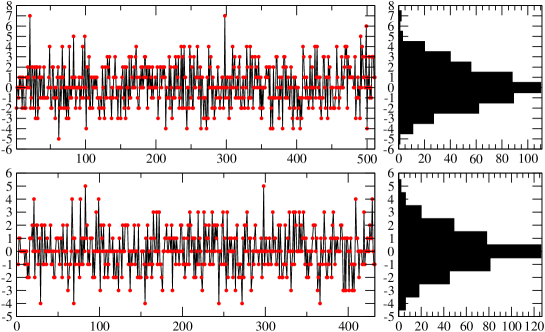
Figure 1: The time history of $Q$ for $\beta=5.9$, m=1 (bottom), and m=1.5 (top).

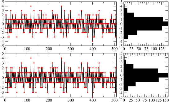
Figure 2: The time history of $Q$ for $\beta=6.0$, m=1 (bottom), and m=1.5 (top).

The time-history of the topological charge for several values of $\beta$ and $m$ are shown in Fig. 1, 2, where one can see that the algorithm does tunnel from one topological sector to the other and that the distribution of values is symmetric and peaked around zero. It is also clear from the figures that the separation between the measurements is large enough to provide statistically independent data. At larger $\beta$, the topological charge distributions are narrower, as one would expect from semi-classical arguments. Comparing the histograms at different values of $m$, we see that, as $m$ is increased, the charge distribution broadens.

The mass dependence of the topological susceptibility, obtained from a spectral flow analysis, is shown in Fig. 3.

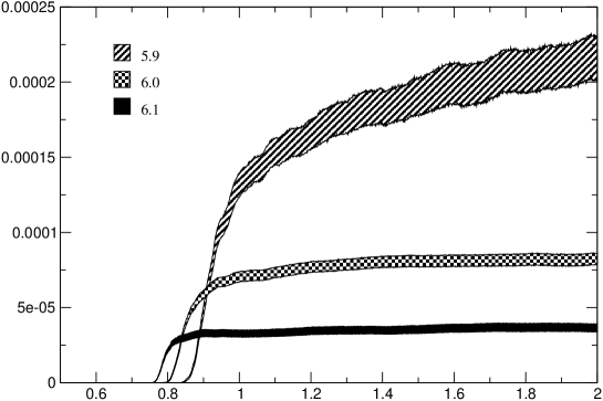
Figure 3: Topological susceptibility $\chi_{L}$ as a function of $m$ for $\beta=5.9$ (top), $6.0$ (middle), and $6.1$ (bottom).

We observe a large effect at lower values of $\beta$, where the value of topological susceptibility as a function of $m$ shows a plateau within the statistical errors only for $m\mathrel{\hbox to0.0pt{\lower 3.0pt\hbox{$\mathchar 536\relax$}\hss}\raise 2.0pt\hbox{$\mathchar 318\relax$}}1.5$. For $m\simeq 1.0$, the value of the susceptibility is about 75% of the asymptotic result. For $\beta\geq 6.0$, the same plateau starts for $m\mathrel{\hbox to0.0pt{\lower 3.0pt\hbox{$\mathchar 536\relax$}\hss}\raise 2.0pt\hbox{$\mathchar 316\relax$}}1.0$. Such dependence should be taken into account in studies performed at fixed value of $m$. The density of crossings vs. $m$ is reported in Fig. 4; the expected behaviour is clearly observed. The value of $m_{1}$, where the gap closes, decreases as the continuum limit is approached; in the same limit, the level crossings cluster in the vicinity of $m_{1}$, so that the topological susceptibility becomes effectively $m$-independent. For lattice sizes $L\mathrel{\hbox to0.0pt{\lower 3.0pt\hbox{$\mathchar 536\relax$}\hss}\raise 2.0pt\hbox{$\mathchar 318\relax$}}0.9{\rm fm}$, our results compare well with those presented in Ref. [26], where finite size effects were observed on smaller lattices, e.g. on a $8^{3}\times 16$ at $\beta=6.0$.

Figure 4: Distribution of level crossings as a function of $m$ for $\beta=5.9$ (bottom), $6.0$ (middle), and $6.1$ (top).

The data obtained from the overlap can be compared with those obtained by a cooling algorithm on the same configurations. Data in Tab. 2 show that the discrepancy between the fermionic and bosonic estimator of the topological charge ($Q_{f}$ and $Q_{g}$, respectively) decreases as the continuum limit is approached. The distribution of $\Delta Q=Q_{g}-Q_{f}$ is reported in Fig. 5 for $m=1$ and $\beta=5.9$ and $6.0$. For $\beta=6.0$, the agreement of the two methods at $m=1$ is around 90%; a comparison of the two values of $\beta$ shows that the discrepancy between the two methods decreases as the continuum limit is approached, consistently with the scenario outlined in Ref. [31]. The agreement between the two results is also reassuring as far as finite size effects are concerned. Indeed, the high statistics results obtained in Ref. [16] with a cooling technique show that the finite size effects on the topological susceptibility at the values of $\beta$ considered in this work are of the order of a few percent. If the agreement between the two methods is not a coincidence, the cooling and the fermionic estimators are expected to display similar finite size effects, which are known to be well below the statistical accuracy achieved in this work.

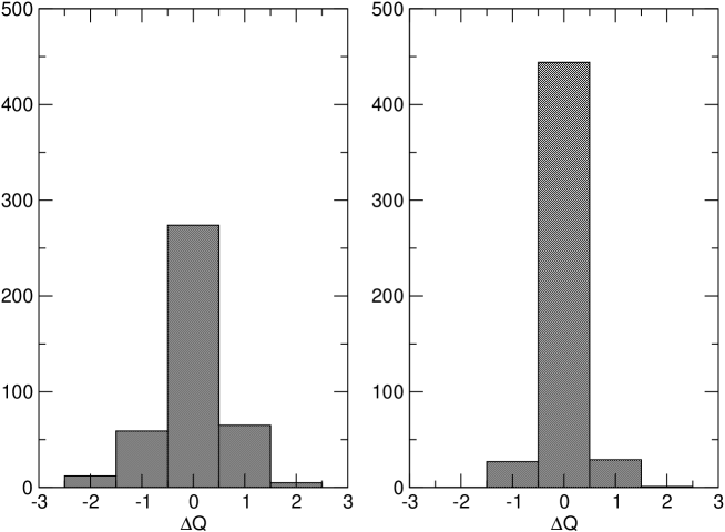
Figure 5: Distribution of the difference $\Delta Q=Q_{g}-Q_{f}$ for $m=1$, $\beta=5.9$ (left), and $6.0$ (right).

In Fig. 6, we report the rate of discrepancies between the fermionic and gluonic definitions as a function of $m$, for the three values of the coupling. It is interesting to note that the best agreement is obtained at intermediate values of $m$. The level crossings in the vicinity of the threshold $m_{1}$ are the ones that build the topological charge detected by the cooling method. Level crossings further away from $m_{1}$ correspond to topological excitations that are eliminated by the cooling process, suggesting that they are associated to modes at the scale of the cut-off.

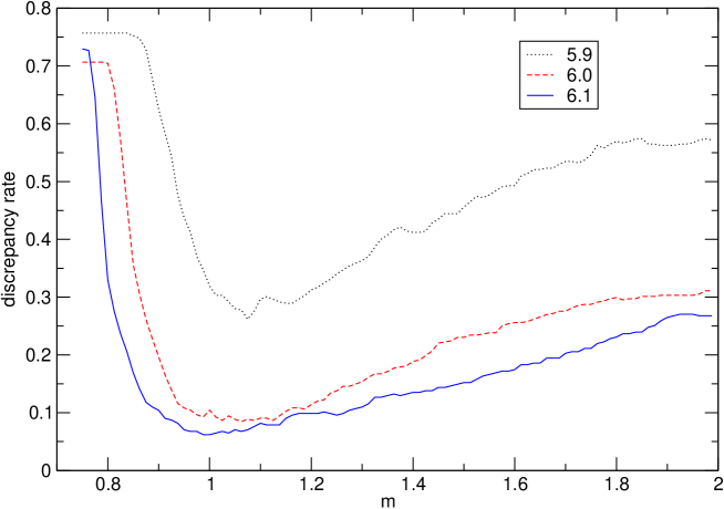
Figure 6: Discrepancy rate between the gluonic and fermionic determinations of the topological charge as a function of $m$ for $\beta=5.9$ (top), $6.0$ (middle), and $6.1$ (bottom).

3.2 Extrapolation to the continuum limit

In order to study the extrapolation to the continuum limit, we build the adimensional ratios $C_{\sigma}=\chi_{L}/\sigma^{2}$ and $C_{r_{0}}=\chi_{L}r_{0}^{4}$, and report their values in Tab. 3. To compare directly with other works, we also compute the fourth root of the scaling ratios. The scaling ratio $C_{\sigma}$ is displayed in Fig. 7 as a function of $a^{2}\sigma$, since the leading scaling corrections are expected to be $\mathcal{O}(a^{2})$.

Table 3: The scaling ratios $C_{\sigma}$, $C^{1/4}_{\sigma}$, $C_{r_{0}}$, and $C^{1/4}_{r_{0}}$.

$\beta$	method	$m$	$C_{\sigma}$	$C^{1/4}_{\sigma}$	$C_{r_{0}}$	$C^{1/4}_{r_{0}}$
5.9	overlap	1	0.0273(23)	0.407(9)	0.0509(32)	0.475(8)
	overlap	1.5	0.0390(37)	0.445(10)	0.0727(52)	0.519(8)
	cooling		0.0308(26)	0.419(9)	0.0574(36)	0.489(8)
	Ref. [16]		0.0334(9)	0.428(3)	0.0622(4)	0.499(1)
6.0	overlap	1	0.0300(19)	0.416(7)	0.0581(25)	0.491(5)
	overlap	1.5	0.0343(25)	0.430(8)	0.0664(33)	0.508(6)
	cooling		0.0311(19)	0.420(7)	0.0602(25)	0.495(5)
	Ref. [16]		0.0312(7)	0.420(3)	0.0604(4)	0.496(1)
6.1	overlap	1	0.0260(26)	0.402(10)	0.0515(38)	0.476(9)
	overlap	1.5	0.0280(28)	0.409(10)	0.0555(42)	0.485(9)
	cooling		0.0282(27)	0.410(10)	0.0558(41)	0.486(8)
	Ref. [16]		0.0308(7)	0.419(4)	0.0611(10)	0.497(2)

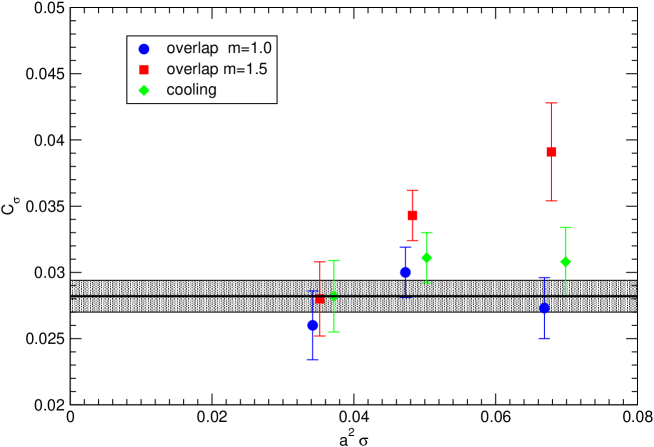
Figure 7: The scaling ratio $C_{\sigma}$ as a function of $a^{2}\sigma$. The grey band is the result of the continuum extrapolation in Ref. [16].

The data at $m=1$ do not display any sizeable dependence on $a^{2}$, and a naive extrapolation can be obtained simply by quoting an interval such that all data points are included:

$$C_{\sigma}(\beta\to\infty)=0.029\pm 0.05$$ (21)

Consistently with the fact that the $m$-dependence becomes negligible as $\beta$ is increased, as shown in Fig. 3, the data point at $m=1.5$ and $\beta=6.1$ is included in the above interval.

Alternatively, one can take a continuum limit by fitting the data either to a constant, or a linear function. We obtain:

$$C_{\sigma}(\beta\to\infty) = 0.028\pm 0.02~{}~{}~{}~{}\mathrm{(constant)}$$ (22)

$$C_{\sigma}(\beta\to\infty) = 0.026\pm 0.04~{}~{}~{}~{}\mathrm{(linear)}$$ (23)

where the errors on the fitted parameters are estimated using a bootstrap method. The results obtained are in excellent agreement with previous determinations.

It is clear from Fig. 7 that there are sizeable scaling violations for $m=1.5$, such that the extrapolated results in the continuum limit are dominated by the large value at $\beta=5.9$. In order to get a more reliable result one should increase the statistics for the current data and add another point closer to the continuum limit, e.g. at $\beta=6.2$. This would require a larger lattice in order to avoid finite size effects, an effort that is beyond the scope of this work.

Data obtained from overlap operators with different values of $m$ can be put together in a single constrained fit, assuming that they all yield the same continuum limit, and allowing for quartic terms in the extrapolation:

$$C_{\sigma,m}(\beta)=C_{\sigma}(\beta\to\infty)+c_{1,m}a^{2}(\beta)+c_{2,m}a^{4}(\beta)$$ (25)

with $c_{0}$ independent on $m$. Such a procedure allows a non-linear dependence on $a^{2}$ to be taken into account; however, one should remember that the data used for the simultaneous fit are not independent, so that the bootstrap errors on the fitted values should only be taken as an indication. The result of the constrained fit is:

$$C_{\sigma}(\beta\to\infty)=0.025{}^{+2}_{-10}$$ (26)

As a consistency check, one can fix $C_{\sigma}(\beta\to\infty)$ to the value obtained above, e.g. by fitting the data at $m=1$ to a constant, and fit the data for both values of $m$ to Eq. (25) with only four parameters. The data fit this ansatz with a $\chi^{2}/\mathrm{dof}\approx 1$.

The same analysis can be performed for the scaling ratio $C_{r_{0}}$. The reference scale $r_{0}$ has been computed to great accuracy and a formula for the interpolation to arbitrary values of $\beta\in\left[5.7,6.57\right]$ does exist [36]. The use of $r_{0}$ for the scaling analysis guarantees a greater uniformity when trying to unify data from different studies [28]. The results of the fits are:

$$C_{r_{0}}(\beta\to\infty) = 0.054(3)~{}~{}~{}~{}~{}~{}~{}\mathrm{for}\ m=1.0,\ \mathrm{constant\ fit}$$ (27)

$$C_{r_{0}}(\beta\to\infty) = 0.055(8)~{}~{}~{}~{}~{}~{}~{}\mathrm{for}\ m=1.0,\ \mathrm{linear\ fit}$$ (28)

A naive extrapolation, which includes all the results for $m=1$, yields $C_{r_{0}}=0.055(10)$.

Combining the two determinations, we obtain:

$$\chi^{1/4}=188\pm 12\pm 5\,{\rm MeV}$$ (29)

where the first error is statistical and the second corresponds to the two different methods of setting the scale.

4 Conclusions

Using a fermionic estimator to compute the topological susceptibility in the continuum limit has some appealing features: the chiral symmetry at finite lattice spacing fixes the renormalization of the lattice operators, so that no renormalization constants are needed. This is also the case for determinations based on the cooling technique; nonetheless the latter are based on assumptions on the separation of gaussian and topological modes.

However, the fermionic method also introduces systematic errors, which one would like to control: the dependence on the mass parameter $m$, that appears in the definition of the overlap, finite size effects, and the size of the lattice artifacts at current values of the coupling.

In agreement with theoretical arguments and previous numerical investigations, we find that the topological suceptibility does vary with $m$ at small values of $\beta$, and that this dependence disappears as the continuum limit is approached. Studies using the overlap at fixed value of $m$ should take this source of systematic error into account, even though we expect the magnitude of the systematics to depend on the observables. Finally, comparison with results obtained using a cooling procedure on the same configurations shows that the two determinations agree in the continuum limit. For values of $m\mathrel{\hbox to0.0pt{\lower 3.0pt\hbox{$\mathchar 536\relax$}\hss}\raise 2.0pt\hbox{$\mathchar 318\relax$}}1.2$, the fermionic method detects topological charges that are smoothed away by the cooling procedure, which could be related to degrees of freedom at the cut-off scale.

On our lattices of linear size $L\simeq 1{\rm fm}$, the comparison with cooling suggests that finite size effects are small compared with our current statistical error.

Our results for the continuum extrapolation are compatible with other determinations. In order to further constrain our extrapolation, one more point at $\beta=6.2$, larger lattices, and higher statistics are needed. Moreover, improved actions could be used to reduce lattice artifacts and possibly achieve a faster convergence towards the continuum limit. Based on our experience, a precise determination of the continuum limit extrapolation is well within reach.

If one is only interested in the topological charge and susceptibility, a spectral flow analysis is sufficient and can be implemented quite efficiently using the procedure outlined above. Instead studies of the overlap operator are needed if one wants to investigate the correlator of the topological density $\langle q_{L}(x)q_{L}(0)\rangle$.

- [1] S. Weinberg, Phys. Rev. D 11 (1975) 3583.
- [2] G. ’t Hooft, Phys. Rev. Lett. 37 (1976) 8.
- [3] G. ’t Hooft, Nucl. Phys. B 72 (1974) 461.
- [4] E. Witten, Nucl. Phys. B 156 (1979) 269.
- [5] G. Veneziano, Nucl. Phys. B 159 (1979) 213.
- [6] R. J. Crewther, Riv. Nuovo Cim. 2N8 (1979) 63.
- [7] A. S. Kronfeld, DESY-87-152
- [8] M. Campostrini, A. Di Giacomo and H. Panagopoulos, Phys. Lett. B 212 (1988) 206.
- [9] M. Campostrini, A. Di Giacomo, H. Panagopoulos and E. Vicari, Nucl. Phys. B 329 (1990) 683.
- [10] A. Di Giacomo and E. Vicari, Phys. Lett. B 275 (1992) 429.
- [11] B. Alles, M. Campostrini, A. Di Giacomo, Y. Gunduc and E. Vicari, Phys. Rev. D 48 (1993) 2284 [arXiv:hep-lat/9302004].
- [12] B. Alles, M. D’Elia and A. Di Giacomo, Nucl. Phys. B 494 (1997) 281 [arXiv:hep-lat/9605013].
- [13] M. Teper, Phys. Lett. B 171 (1986) 81.
- [14] M. Teper, Phys. Lett. B 171 (1986) 86.
- [15] P. de Forcrand, M. Garcia Perez and I. O. Stamatescu, Nucl. Phys. B 499 (1997) 409 [arXiv:hep-lat/9701012].
- [16] L. Del Debbio, H. Panagopoulos and E. Vicari, JHEP 0208 (2002) 044 [arXiv:hep-th/0204125].
- [17] P. H. Ginsparg and K. G. Wilson, Phys. Rev. D 25 (1982) 2649.
- [18] R. Narayanan and H. Neuberger, Phys. Rev. Lett. 71 (1993) 3251 [arXiv:hep-lat/9308011].
- [19] R. Narayanan and H. Neuberger, Nucl. Phys. B 443 (1995) 305 [arXiv:hep-th/9411108].
- [20] P. Hasenfratz, Nucl. Phys. B 525 (1998) 401 [arXiv:hep-lat/9802007].
- [21] M. Luscher, Phys. Lett. B 428 (1998) 342 [arXiv:hep-lat/9802011].
- [22] P. Hasenfratz, V. Laliena and F. Niedermayer, Phys. Lett. B 427 (1998) 125 [arXiv:hep-lat/9801021].
- [23] L. Giusti, G. C. Rossi, M. Testa and G. Veneziano, “The U(1)A problem on the lattice with Ginsparg-Wilson fermions,” Nucl. Phys. B 628 (2002) 234 [arXiv:hep-lat/0108009].
- [24] L. Giusti, “Exact chiral symmetry on the lattice: QCD applications,” arXiv:hep-lat/0211009, and references therein.
- [25] A. Ali Khan et al. [CP-PACS Collaboration], Phys. Rev. D 64 (2001) 114501 [arXiv:hep-lat/0106010].
- [26] R. G. Edwards, U. M. Heller and R. Narayanan, Nucl. Phys. B 535 (1998) 403 [arXiv:hep-lat/9802016].
- [27] C. Gattringer, R. Hoffmann and S. Schaefer, Phys. Lett. B 535 (2002) 358 [arXiv:hep-lat/0203013].
- [28] P. Hasenfratz, S. Hauswirth, T. Jorg, F. Niedermayer and K. Holland, Nucl. Phys. B 643 (2002) 280 [arXiv:hep-lat/0205010].
- [29] T. DeGrand and U. M. Heller [MILC collaboration], Phys. Rev. D 65 (2002) 114501 [arXiv:hep-lat/0202001].
- [30] R. G. Edwards, U. M. Heller, J. E. Kiskis and R. Narayanan, Phys. Rev. D 61 (2000) 074504 [arXiv:hep-lat/9910041].
- [31] N. Cundy, M. Teper and U. Wenger, Phys. Rev. D 66 (2002) 094505 [arXiv:hep-lat/0203030].
- [32] P. Hernandez, K. Jansen and M. Luscher, Nucl. Phys. B 552 (1999) 363 [arXiv:hep-lat/9808010].
- [33] J. van den Eshof, A. Frommer, T. Lippert, K. Schilling and H. A. van der Vorst, Comput. Phys. Commun. 146 (2002) 203 [arXiv:hep-lat/0202025].
- [34] L. Giusti, C. Hoelbling, M. Luscher and H. Wittig, Comput. Phys. Commun. 153 (2003) 31 [arXiv:hep-lat/0212012].
- [35] T. Kalkreuter and H. Simma, Comput. Phys. Commun. 93 (1996) 33 [arXiv:hep-lat/9507023].
- [36] M. Guagnelli, R. Sommer and H. Wittig [ALPHA collaboration], Nucl. Phys. B 535 (1998) 389 [arXiv:hep-lat/9806005].
- [37] H. Neuberger, Phys. Rev. D 61 (2000) 085015 [arXiv:hep-lat/9911004].
- [38] M. Luscher, Nucl. Phys. Proc. Suppl. 106 (2002) 21 [arXiv:hep-lat/0110007].