Application of Maximum Entropy Method to Lattice Field Theory with a Topological Term

Abstract

In Monte Carlo simulation, lattice field theory with a $\theta$ term suffers from the sign problem. This problem can be circumvented by Fourier-transforming the topological charge distribution $P(Q)$. Although this strategy works well for small lattice volume, effect of errors of $P(Q)$ becomes serious with increasing volume and prevents one from studying the phase structure. This is called flattening. As an alternative approach, we apply the maximum entropy method (MEM) to the Gaussian $P(Q)$. It is found that the flattening could be much improved by use of the MEM.

1 INTRODUCTION

It is well known that non-perturbative properties of the strong interaction are relevant to the dynamics at low energy such as the U(1) problem. Although a $\theta$ term is deeply associated with the non-perturbative properties, it is indicated experimentally that the effect of the $\theta$ term is suppressed. This is the strong CP problem. The existence of the $\theta$ term also opens the possibility of rich phase structures in $\theta$ space. So it is important to study the dynamics of QCD with the $\theta$ term.

The $\theta$ term makes Boltzmann weight complex in the euclidean path integral formalism. This makes it difficult to perform Monte Carlo simulation. This problem can be circumvented by Fourier-transforming the topological charge distribution $P(Q)$. The partition function ${\cal Z}(\theta)$ is given as

$${\cal Z}(\theta)\equiv\sum_{Q}P(Q)e^{i\theta Q},$$ (1)

where $P(Q)$ is given as

$$P(Q)\equiv\frac{\int[{\cal D}\phi]_{Q}e^{-S(\phi)}}{\int{\cal D}\phi e^{-S(\phi)}}.$$ (2)

The measure $[{\cal D}\phi]_{Q}$ represents that the integral is restricted to configurations of the field $\phi$ with the topological charge $Q$, and $S$ denotes an action.

Although this algorithm works well for small lattice volume[1, 2, 3, 4], the effect of errors of $P(Q)$ becomes serious and disturbs the behavior of ${\cal Z}(\theta)$ as volume increases. In fact, a fictitious signal of a phase transition was observed due to the errors of $P(Q)$[5, 6]. This is called flattening. The flattening could be remedied by increasing statistics, but it is hopeless because exponentially increasing statistics are needed with increasing volume. So we do need an alternative way${}^{\cite[cite]{[\@@bibref{}{rf:ADGL}{}{}]}}$ to calculate ${\cal Z}(\theta)$ properly.

In this talk, we use the inverse Fourier transform and apply the maximum entropy method (MEM). As a model, we employ the Gaussian $P(Q)$.

2 MODEL AND FLATTENING

The Gaussian $P(Q)$ is parametrized as follows;

$$P(Q)\propto e^{-\frac{c}{V}Q^{2}}.\;\;\;(c,V:\mbox{parameters})$$ (3)

This model realizes in the 2-d U(1) gauge model, the strong coupling limit of the CP^N-1 model and so on. The parameters $c$ and $V$ are regarded as a constant depending on the coupling constant and a volume in the U(1) gauge model, respectively. For our analysis, we use mock data by adding the Gaussian noise with the variance of $\delta\times P(Q)$ to the Gaussian $P(Q)$.

Fig. 1 shows the free energy density, $f(\theta)\equiv-\frac{1}{V}\log{\cal Z}(\theta)$, obtained by Fourier-transforming numerically the mock data for various volumes.

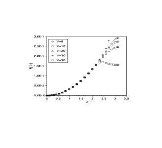
Figure 1: Free energy density $f(\theta)$ for various volumes, $c=7.42$ and $\delta=1/400$.

As $V$ increases, already at $V=30$, $f(\theta)$ cannot be calculated correctly because of errors of $P(Q)$ in Fig. 1. Especially at $V=50$, $f(\theta)$ becomes flat for $\theta\hskip 3.00003pt\raisebox{1.72218pt}{$>$}\raisebox{-3.01385pt}{$\sim$}\hskip 3.00003pt2.3$ and gives a fictitious signal of a first-order phase transition at $\theta\simeq 2.3$. This is nothing but the flattening. Since the flattening is characteristic of the Fourier transform procedure, an alternative way should be employed to calculate $f(\theta)$ properly.

3 MAXIMUM ENTROPY METHOD

In this talk, the inverse Fourier transform is used in the analysis. In this case, the number of degrees of freedom of $Q$, $N_{q}$, is smaller than that in $\theta$ space, $N_{\theta}$, and the analysis by use of the $\chi^{2}$-fit suffers from the ill-posed problem. In order to circumvent this problem, we use the MEM, which is effective for such the issue.

The MEM is based on the Bayes’ theorem in the probability theory. For our case, probability ${\rm prob}({\cal Z}(\theta)|P(Q),I)$ is considered, which is the probability that ${\cal Z}(\theta)$ is realized when data of $\{P(Q)\}$ and information $I$ are given. The information $I$ represents our state of knowledge about ${\cal Z}(\theta)$. In this case, we impose a criterion that ${\cal Z}(\theta)>0$.

The probability ${\rm prob}({\cal Z}(\theta)|P(Q),I)$ is written in terms of $\chi^{2}$ and the entropy $S$;

$${\rm prob}({\cal Z}(\theta)|P(Q),I)\propto\exp\bigl{\{}-\frac{1}{2}\chi^{2}+\alpha S\bigr{\}}\equiv e^{W({\cal Z})},$$ (4)

where $\alpha$ is a real-positive parameter. Conventionally the Shannon-Jaynes entropy $S$ is employed[8, 9].

$$S=\int^{\pi}_{-\pi}d\theta\biggl{[}{\cal Z}(\theta)-m(\theta)-{\cal Z}(\theta)\log\frac{{\cal Z}(\theta)}{m(\theta)}\biggr{]},$$ (5)

where $m(\theta)$ is called default model which reflects our state of knowledge about ${\cal Z}(\theta)$. Namely, our task is to explore the image ${\hat{\cal Z}}(\theta)$ such that ${\rm prob}({\cal Z}(\theta)|P(Q),I)$ is maximized by following the three steps[8, 9];

1. Maximizing $W({\cal Z})$ for a given $\alpha$:

   $$\frac{\delta W({\cal Z})}{\delta{\cal Z}(\theta)}\Biggm{|}_{{\cal Z}={\cal Z}^{(\alpha)}}=0.$$ (6)

2. Averaging ${\cal Z}^{(\alpha)}(\theta)$ to calculate the best image ${\hat{\cal Z}}(\theta)$ which maximizes ${\rm prob}({\cal Z}(\theta)|P(Q),I)$:

   $${\hat{\cal Z}}(\theta)\simeq\int d\alpha~{}{\rm prob}(\alpha|P(Q),I){\cal Z}^{(\alpha)}(\theta),$$ (7)

3. Error estimation.

4 RESULTS

In our analysis, the Gaussian $P(Q)$ is used as a test. It is a good laboratory to investigate how the flattening is improved, because the corresponding partition function ${\cal Z}_{{\rm pois}}(\theta)$ is calculated by use of the Poisson’s sum formula analytically. We perform the analysis for various parameters $c$, $V$, $\delta$. Here we fix $c=7.42$, $V=50$ and $\delta=1/400$. The number of data set is 30. Three default models are employed: (i) constant type; $m(\theta)=1.0$, (ii) strong coupling region type; $m(\theta)=(\frac{2}{\theta}\sin\frac{\theta}{2})^{V}$, (iii) Gaussian type; $m(\theta)=\exp\bigl{\{}-\frac{\log 10}{\pi^{2}}\gamma\theta^{2}\bigr{\}}$, where the parameter $\gamma$ is varied from 4 to 8. In the analysis, it is non-trivial to find a solution due to $N_{q}<N_{\theta}$ and the singular value decomposition is employed. In order to calculate image ${\hat{\cal Z}}(\theta)$ with high precision, the Newton method is used with quadruple precision.

Firstly, in order to find a solution which approximately agrees with the exact ${\cal Z}_{{\rm pois}}(\theta)$, analyses are performed by using the three default models for various $\alpha$ by step 1.

Figure 2: ${\cal Z}^{(\alpha)}(\theta)$ for data at $V=50$ with flattening. As a comparison, the result of Fourier transform($\circ$) and ${\cal Z}_{{\rm pois}}(\theta)$($\bullet$) are also displayed.

Fig. 2 shows the results. Note that all the results of the MEM are free from the flattening. Results of the constant type at $\alpha=300$ and the Gaussian one with $\gamma=6$ at $\alpha=2000$ approximately agree with the exact ${\cal Z}_{{\rm pois}}(\theta)$.

In order to investigate whether these solutions are favored probabilistically, we calculate ${\hat{\cal Z}}(\theta)$ following step 2 and also estimate these errors by step 3. We find that ${\hat{\cal Z}}(\theta)$ given by the Gaussian default model with $\gamma=6$ is the most favorite image in the current analysis.

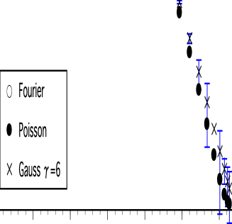
Figure 3: ${\hat{\cal Z}}(\theta)$ given by the Gaussian type with $\gamma=6$.

The result is shown in Fig. 3. The result is free from the flattening and consistent with ${\cal Z}_{{\rm pois}}(\theta)$. Hence we conclude that the MEM works for the $\theta$ term and reproduces the reasonable image[10].

5 SUMMARY

In this talk, we applied the MEM to mock data of the Gaussian $P(Q)$ and showed that the flattening is much improved by use of the MEM.

The next task is to apply the MEM to more realistic models.

References

- [1] G. Bhanot, E. Rabinovici, N. Seiberg and P. Woit, Nucl. Phys. B230[FS10] (1984), 291.
-
[2]
U. -J. Wiese, Nucl. Phys. B318 (1989), 153.
W. Bietenholtz, A. Pochinsky and U. -J. Wiese, Phys. Rev. Lett. 75 (1995), 4524. - [3] A. S. Hassan, M. Imachi, N. Tsuzuki and H. Yoneyama, Prog. Theor. Phys. 95 (1995), 175.
- [4] R. Burkhalter, M. Imachi, Y. Shinno and H. Yoneyama, Prog. Theor. Phys. 106 (2001), 613.
- [5] J. C. Plefka and S. Samuel, Phys. Rev. D56 (1997), 44.
- [6] M. Imachi, S. Kanou and H. Yoneyama, Prog. Theor. Phys. 102 (1999), 653.
- [7] V. Azcoiti, G. Di Carlo, A. Galante and V. Laliena, Phys. Rev. Lett 89 (2002), 141601.
- [8] R. K. Bryan, Eur. Biophys. J 18 (1990), 165.
- [9] M. Asakawa, T. Hatsuda and Y. Nakahara, Prog. Part. Nucl. Phys. 46 (2001), 459.
- [10] M. Imachi, Y. Shinno and H. Yoneyama, in preparation.