1.5

Improvement and Analytic Techniques in Hamiltonian Lattice Gauge Theory

Abstract

This thesis is concerned with two topics in Hamiltonian lattice gauge theory (LGT): improvement and the application of analytic techniques. On the topic of improvement, we develop a direct method for improving lattice Hamiltonians for gluons, in which linear combinations of gauge invariant lattice operators are chosen to cancel the lowest order discretisation errors. A number of improved Hamiltonians are derived and the level of improvement tested for the simple cases of U(1) in 3+1 dimensions and SU(2) in 2+1 dimensions. In each case the improved calculations are closer to the continuum limit, when working at a given lattice spacing, than their unimproved counterparts.

On the topic of analytic methods, we extend the techniques that have been used in 2+1 dimensional SU(2) variational calculations for many years, to the general case of SU($N$). For this purpose a number of group integrals are calculated in terms of Toeplitz determinants. As generating functions these group integrals allow the calculation of all matrix elements appearing in variational glueball mass calculations in 2+1 dimensions. Making use of these analytic techniques, the lowest five glueball masses, or massgaps, in various symmetry sectors are calculated, with improved and unimproved Hamiltonians, for $2\leq N\leq 5$. For simplicity, a minimisation basis containing only rectangular states is used. Large scaling regions are obtained for each of the five lowest mass states in the $J^{PC}=0^{++}$ and $0^{--}$ sectors. The results are comparable to competing calculations. However, the enumeration of the states obtained requires further work.

The large $N$ limit of the glueball mass spectrum is also explored. Making use of analytic variational techniques, glueball mass calculations with $N$ as large as 25 are carried out on a desktop computer and the results extrapolated accurately to the $N\rightarrow\infty$ limit. Evidence of leading order $1/N^{2}$ finite $N$ corrections is obtained for a number of excited states. An interesting empirical observation is made which demonstrates a close similarity between the glueball mass spectrum and the simple harmonic oscillator spectrum in 2+1 dimensions.

We finish with a feasibility study of applying analytic Hamiltonian techniques in 3+1 dimensional calculations. After developing analytic techniques specific to 3+1 dimensions, we study the variational glueball mass spectrum for SU($N$) on a single cube, with a minimisation basis containing only two states. Memory limitations do not allow calculations with $N\geq 8$. We observe promising signs of an approach to asymptotic scaling in the $1^{+-}$ sector as $N$ is increased, warranting larger volume studies with additional states in the minimisation basis.

Declaration

  This is to certify that

• this thesis comprises only my original work,

• due acknowledgement has been made in the text to all other material used,

• this thesis is less than 100,000 words in length, exclusive of table, maps, bibliographies, appendices and footnotes.

…………………………………

…………………………………
 

Chapter 1 Introduction

1.1 Historical Background

Quantum chromodynamics (QCD) is the accepted theory of high energy strong interactions. It is the gauge theory describing the interactions of coloured particles, quarks and gluons, which are commonly accepted to be the fundamental degrees of freedom of hadronic matter.

The non-abelian nature of QCD results in a collection of non-trivial complications when compared to the archetypal gauge theory quantum electrodynamics (QED). Most serious is the phenomenon of asymptotic freedom which dictates that the QCD coupling constant, $g^{2}$, is not in fact constant. Rather it depends on the energy scale of the process in question. The calculation of the one-loop $\beta$ function Gross and Wilczek (1973); Politzer (1973) demonstrated that the QCD coupling constant is small only for high energy processes; a fact observed in experiment. This discovery was instrumental in the establishment of QCD as a theory of strong interactions.

Asymptotic scaling poses a serious problem to quantitative tests of QCD. The traditional perturbative techniques used in high precision tests of QED rely on expansions about a small coupling constant. Consequently such techniques are only applicable to high energy QCD processes. Perturbative QCD has had a great deal of success explaining such processes.

The first quantitative demonstration of the validity of perturbative QCD was in the violation of Bjorken scaling in deep-inelastic lepton-hadron scattering (for example see Ref. Gribov and Lipatov (1972)). More recently high order QCD calculations of jet rates in hadron colliders have shown impressive agreement with experimental data. Less striking tests of perturbative QCD have been made in the analysis of $\tau$ lepton decays, heavy-quarkonium decay and also in $e^{+}e^{-}$ collisions. For a recent review see Ref. Hagiwara et al. (2002).

For low energy processes the QCD coupling constant is large. Consequently traditional perturbative techniques can not be used to test the validity of QCD in this regime. A great deal of interesting physics appears in this nonperturbative regime. One would like to test whether the same theory that successfully explains a broad range of high energy processes also gives rise to quark confinement, provides a mechanism for chiral symmetry breaking, gives rise to the correct values for the hadronic mass spectrum and explains other low-energy phenomena. Without the use of non-perturbative techniques the situation is dire. One cannot calculate such mental quantities as the masses of mesons and baryons even if given the coupling constant and the constituent quark masses. The need to probe the low-energy regime of QCD has given rise to many QCD motivated models Chodos et al. (1974); Cornwall and Soni (1983); Isgur and Paton (1985); Johnson and Teper (2002). However, only one first principles approach to nonperturbative QCD is currently known and that is lattice gauge theory (LGT).

LGT was originally developed in the Lagrangian formulation by Wilson in 1975 Wilson (1974). A year later the corresponding Hamiltonian formulation was published by Kogut and Susskind Kogut and Susskind (1975). The basic approximation of LGT is the replacement of continuous and infinite space-time by a discrete lattice of sites and links. The essential difference between the Hamiltonian and Lagrangian formulations is that in the former time is left continuous. Using LGT one can presumably calculate the full range of hadronic properties from mass spectra and wave functions to decay constants and matrix elements. The hadronic matrix elements appearing in the weak decays of hadrons are of particular interest. Phenomenologists are waiting for lattice estimates to such matrix elements in order to improve the theoretical understanding of the CKM matrix Beneke (2002); Ryan (2002). Another area of recent interest has been in the study of QCD in extreme conditions. A knowledge of the phase diagram of QCD is relevant to the understanding of high density quark systems such as the early universe, neutron stars and heavy ion collisions. The scope of LGT is summarised in Ref. Gupta (1997).

In practice LGT cannot, at this stage, predict the complete range of hadronic phenomena. The major stumbling block is the requirement of time on the largest supercomputers in existence to calculate basic quantities with accuracy. In the early days of LGT strong coupling expansions in the Hamiltonian approach provided compelling evidence for the confinement of quarks by showing that the potential energy between two infinitely heavy quarks grows linearly with their separation Kogut and Susskind (1975); Kogut (1980). This was without the complication of dynamical quarks and in the strong coupling limit which is far from the real world physics of the continuum. The inclusion of two flavours of quarks and the extension to physical couplings came much later and required the numerical techniques of Lagrangian LGT. The qualitative result of the strong coupling expansions did not however change (for example see Ref. Bali et al. (2000) and references within).

Most LGT calculations to date have been performed using Monte Carlo techniques in the Lagrangian approach. Until recently most simulations used the so called quenched approximation in which the vacuum polarization effects of the QCD vacuum are explicitly removed. The calculation of certain hadron masses are within 10% of the experimentally observed results using the quenched approximation Aoki et al. (2000). Calculations utilising full QCD with two flavours of quarks have been performed and show significant improvements over the quenched approximation Yoshie (2002). At this stage the advancement of LGT in the Lagrangian approach is restricted by the available computational resources.

There are some areas of research where progress in the Lagrangian formulation has been significantly slow. Some examples are in calculations involving excited states and the determination of the QCD phase diagram. Such slow progress and the need for significant computational resources in Lagrangian LGT suggests that alternative methods should be pursued in parallel. A viable alternative is Hamiltonian LGT, which may have a number of advantages. It has been suggested that Hamiltonian LGT could more readily handle finite density QCD Gregory et al. (2000). Indeed, the problems encountered in finite density QCD in the Lagrangian formulation has prompted a return to the strong coupling expansions of early Hamiltonian LGT Bringoltz and Svetitsky (2002). Additional areas in which Hamiltonian LGT may have an advantage over the Lagrangian approach are in calculations involving excited sites, time dependent quantities and wave functions. An appealing aspect of the Hamiltonian approach is that it reduces LGT to a many body problem. As such a host of analytic techniques from many body theory are applicable. Techniques such as the coupled cluster method Coester (1958); Coester and Kümmel (1960); Ligterink et al. (2000); McKellar et al. (2000), plaquette expansion Hollenberg (1993, 1994); McIntosh and Hollenberg (2002a, b) and variational methods Arisue et al. (1983); Arisue (1990) have had success in recent years in calculations of glueball masses. These calculations however have been performed without the inclusion of quarks, often in less dimensions that the physical 3+1 and often using lower dimensional gauge groups than the physical case of SU(3).

The self interactions of gluons in QCD allow the existence of massive states containing only gluon degrees of freedom Fritzsch and Gell-Mann (1972); Fritzsch et al. (1973). Although QCD provides a theory of strong interactions we have little understanding of the physical states of the theory. The constituent quark model provides an excellent phenomenological description of meson and baryon spectroscopy. QCD inspired models however predict the existence of other hadrons. These hadrons include not only the glueballs, which are often described as bound states of two and three gluons, but other more exotic states as well. So called hybrid particles, which have both quark and excited gluon degrees of freedom, have been predicted to exist. Until the properties of the physical states of QCD can be reliably calculated, and these calculations stand up to experimental tests, we cannot claim to understand the nonperturbative aspects of QCD. From both theoretical and experimental sides there have been significant developments in the search for glueballs in recent years.

On the theoretical side calculations of the glueball mass spectrum have been dominated by LGT calculations in the Lagrangian approach. The calculations of the last decade are nearing agreement at least for the lowest mass glueballs. The emerging picture is that the scalar glueball with quantum numbers $J^{PC}=0^{++}$ is the lightest with a mass in the range 1.4–1.8 GeV. Interestingly the next lowest mass states in the $PC=++$ sector have spin ordering 2, 3, 1, whereas the ordering in the $PC=-+$ sector is 1, 3, 2, 0. The status of LGT glueball calculations in the Lagrangian approach is reviewed in Refs. Bali (2001) and Morningstar (2002).

On the experimental side progress has been hampered by numerous technical difficulties. Perhaps most significant is the fact that glueballs can mix strongly with nearby $q\bar{q}$ resonances. To search for glueballs one needs to probe glue rich processes. Recent searches have taken place in radiative $J/\psi$ decay, $p\bar{p}$ annihilations and central production in $pp$ collisions. A review of search techniques is presented in Ref. Godfrey and Napolitano (1999). Perhaps the most promising glueball candidates are the $f_{0}(1500)$ and $f_{0}(1710)$ resonances (the subscript denotes the total angular momentum and the argument the mass in MeV). The interpretation of these resonances has been the subject of much debate, particularly with regard to mixing with $q\bar{q}$ states. Some authors argue that the $f_{0}(1500)$ has a dominant glueball contribution while the glueball content of $f_{0}(1710)$ is minimal Amsler (2002); Amsler and Close (1996). Other authors argue the opposite case Lee and Weingarten (2000); Sexton et al. (1995). Improved data from non-appearance searches in $\gamma\gamma$ collisions could possibly resolve this issue Acciarri et al. (2001). The basis for these studies lies in the fact that the glueball to two photon widths are small compared to those of mesons since gluons do not couple directly with photons. Such studies will also be important in the identification of other glueball candidates such as $f_{J}(2220)$ Benslama et al. (2002).

The focus of most of the lattice community, as far as glueballs are concerned, has been the physically interesting case of SU(3) glueballs in 3+1 dimensions. In recent years the study of glueballs belonging to higher dimensional gauge groups in both 2+1 and 3+1 dimensions has received intense interest from the string theory community. The reason for this is that the SU($N$) glueball mass spectrum in the large $N$ limit provides an ideal laboratory for quantitative tests of Maldacena’s conjecture and its later extensions. We defer the discussion of this topic to Section 7.2.

While accurate studies of the SU(3) glueball spectrum in 3+1 dimensions may be some way off in Hamiltonian LGT, studies of the SU($N$) glueball spectrum in 2+1 dimensions are definitely feasible. In fact it appears that the Hamiltonian approach has a distinct advantage over the Lagrangian approach in that excited states are easily accessed. Current Lagrangian calculations have extracted the three lowest mass states in some sectors in the large $N$ limit. With Hamiltonian techniques it is feasible to even triple this number. The accurate simulation of large mass excited states is of immediate interest to QCD inspired models of glueballs such as the bag model Chodos et al. (1974), potential models Cornwall and Soni (1983) and the flux-tube model Isgur and Paton (1985) and its extensions Johnson and Teper (2002). The last of these in fact shows remarkable agreement with the lowest excited state masses calculated on the lattice in 2+1 dimensions for all but the $0^{-+}$ state Johnson and Teper (2002).

The results so far obtained in Lagrangian LGT have been made possible by an extensive improvement programme initiated by Symanzik nearly twenty years ago Symanzik (1983a, b). The formulation of QCD on a lattice introduces errors which can be expressed in powers of the lattice spacing $a$ and the QCD coupling and start at ${\cal O}(a^{2})$. When performing a lattice calculation in the Lagrangian approach the most important factor in determining the computational cost is the lattice spacing. In fact it has been predicted that the cost of a full QCD simulation varies as $a^{-7.5}$ Jegerlehner et al. (2000). Thus it is very important to be able to work on coarse lattices. This of course is a move away from the $a\rightarrow 0$ limit in which the real world physics of the continuum is retrieved. This realisation has motivated the development of improved actions (for a review see Ref. Lepage (1996)). These actions aim to systematically remove the errors caused by placing QCD on a lattice. In practice these actions allow one be closer to the continuum limit when working with a given lattice spacing. The additional computational cost of working with the more complicated improved actions is by far outweighed by the benefits of working on coarse lattices. The development of improved actions has been a crucial factor in the progress of LGT in the last 15 years. It has allowed routine calculations to be performed on work stations and has brought the numerical solution of full QCD tantalisingly close.

In contrast the improvement of Hamiltonian LGT has hardly begun. Perhaps the most comprehensive study into the derivation of improved Hamiltonians to date is due to Luo, Guo, Kröger and Schütte Luo et al. (1999). Their study started with an improved Lagrangian and derived improved Hamiltonians with the standard transfer matrix and Legendre transformation techniques. Using these techniques it became clear that the construction of an improved kinetic Hamiltonian with a finite number of terms is a non-trivial problem. Using a more direct method improved Hamiltonians can be constructed with relative ease. In this thesis we propose a method for the direct improvement of Hamiltonian LGT which is in the spirit of the original Kogut-Susskind derivation. This topic is the focus of Chapter 3.

We now move on to a description of the outline of the thesis.

1.2 Outline of the Thesis

As a form of introduction, in Chapter 2, the fundamental approximations of LGT are detailed. The basic steps involved in a Hamiltonian lattice calculation are also discussed as well as the important topic of how the real world physics of the continuum is retrieved.

Chapters 3 and 4 are concerned primarily with the topic of improvement. In Chapter 3 we develop a technique which allows the straightforward construction of lattice Hamiltonians for gluons in $d+1$ dimensions. A variety of improved Hamiltonians are derived using this method. These improved Hamiltonians are devoid of the lowest order discretisation errors present in the unimproved Kogut-Susskind Hamiltonian. In Chapter 4 we present some simple checks on improvement for the cases of U(1) in 3+1 dimensions and SU(2) in 2+1 dimensions. In this way we test the level of improvement achieved by a selection of the Hamiltonians derived in Chapter 3.

In Chapter 5 we move on to the topic of analytic methods. Here we introduce techniques which allow analytic lattice calculations of SU($N$) glueball masses in 2+1 dimensions for general $N$. Such techniques extend the SU(2) methods of Arisue Arisue et al. (1983) to the general case of SU($N$). These techniques are applied in Chapter 6 in the calculation of glueball masses in 2+1 dimensions with $2\leq N\leq 5$. Kogut-Susskind, improved and tadpole improved Hamiltonians, all of which are derived in Chapter 3, are used and their results compared.

In Chapter 7 we move on to an analytic study of large $N$ physics on the lattice. Here we study the large $N$ glueball mass spectrum in 2+1 dimensions using the Kogut-Susskind Hamiltonian. Using the analytic techniques of Chapter 5, calculations with $N$ as large as 25 are possible on a desktop computer, allowing an accurate extrapolation to the $N\rightarrow\infty$ limit. Chapters 6 and 7 contain the key results of this thesis.

In Chapter 8 we move on to explore the viability of adapting the analytic techniques, used with success in Chapters 6 and 7, to the physically interesting case of 3+1 dimensions. Here, the difficulties of a move to 3+1 dimensions are discussed. Calculations of glueball masses within a simplistic, one cube, model are presented as a first step in testing the worth of analytic variational techniques in 3+1 dimensions.

Chapter 9 contains a summary of our findings and our conclusions.

Chapter 2 Gauge Theory on a Lattice

2.1 Introduction

In this chapter we describe the basic steps involved in Hamiltonian LGT calculations. Our intention is to introduce the fundamental approximations of LGT and the topics of importance to recovering the real world physics of the continuum. We start with an explanation of how quarks and gluons are put on a lattice in Section 2.2. In this section the important difference in the building blocks of LGT and continuum gauge theory are discussed. We then move on to explain the steps involved in performing a calculation in Hamiltonian LGT. We finish in Section 2.6 with a discussion of the important topic of how the real world physics of the continuum is extracted from a calculation on the lattice.

2.2 The Lattice

The fundamental simplification of LGT is the replacement of continuous and infinite space-time with a finite and discrete lattice of sites and links. A label, $l=(\mbox{\boldmath$x$},i)$, is attached to each link. Here $x$ is the starting point of link $l$ and $i$ its direction. Quark fields are essentially treated in the same way on the lattice as they are in continuum QCD. In both theories they are represented by Grassmann variables. However, in LGT the quark fields are restricted to lattice sites. As in the continuum, the fermion fields can be integrated out of the partition function exactly giving a highly non-local fermion determinant, $\det M$. The calculation of this determinant is the key factor in the computational expense of full QCD simulations in Lagrangian LGT. The quenched approximation, in which the vacuum polarisation effects of the QCD vacuum are explicitly removed, gives $\det M$ a constant value, reducing both the computational expense and the connection to real world physics of LGT. It is in this approximation that the bulk of Lagrangian LGT calculations have been carried out.

In LGT gluons are incorporated differently to continuum gauge theory in order to maintain manifest gauge invariance on the lattice. In continuum SU($N$) gauge theory gluons are represented by the SU($N$) valued fields $A_{\mu}(x)$. In LGT gluons are represented by Wilson lines (or link operators) along the links joining lattice sites. We denote the link operator on link $l$ by $U_{l}$. The link operator on the same link but taken in the opposite direction is given by $U^{\dagger}_{l}$. At times it will be convenient to use the more detailed notation, $U_{i}(\mbox{\boldmath$x$})$, for the link operator on link $l=(\mbox{\boldmath$x$},i)$. It is conventional to represent the link operator by a directed line segment joining the sites $x$ and $\mbox{\boldmath$x$}+a\hat{\mbox{\boldmath$i$}}$, as shown in Fig. 2.1. Here $\hat{\mbox{\boldmath$i$}}$ is a unit vector in the $i$ direction. The details of this construction and precisely how it relates to the continuum theory will be introduced in Section 3.3.2. The fundamental differences between continuum gauge theory and LGT are caricatured in Fig. 2.2. As in Fig. 2.2 it is conventional to denote the lattice spacing by $a$.

Having discussed the fundamental approximation of LGT and briefly introduced its building blocks we now move on to a description of the steps involved in a complete Hamiltonian LGT calculation. The first step is choosing an appropriate lattice.

\psfrag{x+ai}{$\mbox{\boldmath$x$}+a\hat{\mbox{\boldmath$i$}}$}\psfrag{U}{$U_{i}(\mbox{\boldmath$x$})$}\psfrag{x}{$\mbox{\boldmath$x$}$}\psfrag{i}{$i$}\psfrag{j}{$j$}\includegraphics[width=199.16928pt]{link.eps}

Figure 2.1: The link operator.

\psfrag{quark}{quark}\psfrag{gluon}{gluon}\includegraphics[width=256.0748pt]{notlattice1.eps}

(a) Continuum QCD

\psfrag{quark}{quark}\psfrag{gluon}{gluon}\psfrag{a}{$a$}\psfrag{L}{$L$}\includegraphics[width=199.16928pt]{lattice1.eps}

(b) Lattice QCD

Figure 2.2: A cartoon comparing continuum QCD with lattice QCD.

2.3 Defining a Lattice

In Hamiltonian LGT one works on a spatial lattice. The time coordinate remains continuous. Contrastingly, the Lagrangian formulation discretises all dimensions and works in Euclidean space. An obvious advantage of the Hamiltonian approach is that one works with a lattice with one less dimension. The cartoon in Fig. 2.2 illustrates a cubic lattice in three dimensions. LGT is not, however, restricted to 3 dimensions and the lattice itself is not restricted to a cubic arrangement.

For reasons of simplicity, it has been conventional to study LGTs built on cubic lattices. Not a great deal of effort has been devoted to exploring the effect of using lattices with different structures Wichmann (2001). One could however imagine that working on a non-cubic lattice could be advantageous in some situations. For example, if the degrees of freedom were arranged into products of link operators (which is often convenient) around the elementary faces of the lattice (for example squares of side length $a$ in the cubic case), working on non-cubic lattices could be advantageous when the number of faces and number of links need to be related in a precise way to incorporate constraints such as Gauss’ law Ligterink et al. (2000). In this thesis we work on a $d$ dimensional spatial lattice with $d=2$ and 3.

When performing numerical LGT calculations the primary restriction is computer memory. The value of every link operator on the lattice needs to be stored in memory at a given time. Since the number of links on the lattice increases quickly as the volume increases, one is in practice limited to lattices with small volumes. The majority of work in LGT to date has involved small volume numerical simulations in the Lagrangian approach. Typical calculations on supercomputers with speeds of the order of hundreds of gigaflops with two flavours of dynamical quarks are performed on $24^{3}\times 48$ lattices. It has been estimated that with access to a 10 teraflop machine $36^{3}\times 96$ lattices will be able to be used for equivalent calculations with similar effort Jegerlehner et al. (2000).

Variational studies in Hamiltonian LGT in 3+1 dimensions (which go beyond the strong coupling limit), to our knowledge, have only dealt with small lattices; typically with sizes smaller than $6^{3}$ Chin et al. (1988); Long et al. (1988). We discuss the viability of using analytic Hamiltonian techniques in 3+1 dimensions in Chapter 8.

Having defined a lattice we now move on to the important step of constructing a Hamiltonian.

2.4 Constructing a Hamiltonian

When constructing a Hamiltonian on the lattice there are three important points to consider. Firstly, the lattice Hamiltonian must reduce to its continuum counterpart in the limit of vanishing lattice spacing. From here on we refer to this limit as the continuum limit. Secondly, we must incorporate as many symmetries of the continuum theory as possible. Finally, the lattice Hamiltonian must not be prohibitively expensive to use. These points are closely related and often an attempt to address one point is detrimental to another. For example, if one attempts to build a Hamiltonian that is closer to its continuum counterpart for a given lattice spacing, one with a weak dependence on $a$, one is left unavoidably with a more computationally intensive Hamiltonian. Another example relates to restoring rotational symmetry. On the lattice, continuous rotational symmetry is broken down to a discrete analogue which depends on the particular lattice in use. One can attempt to construct Hamiltonians with improved rotational symmetry but again the resulting Hamiltonian is more computationally expensive than the simplest versions.

One symmetry that is essential to incorporate in the lattice Hamiltonian is local gauge invariance. One may ask why it is important to uphold local gauge invariance when other symmetries such as rotational invariance and Lorentz invariance are explicitly broken. The reason lies in the fact that with local gauge invariance upheld the bare gluon mass is zero and the couplings appearing at multiple gluon and gluon-quark vertices are all equal. Without local gauge invariance these couplings would need to be tuned independently in order to retrieve real world physics. This is a complication that would become prohibitively expensive when processes with loop diagrams were taking into consideration.

In building lattice Hamiltonians we have a great deal of freedom. Our only restrictions are gauge invariance and the need to obtain the correct continuum limit. Our approach is to start with gauge invariant lattice operators and form linear combinations such that the correct continuum limit is obtained. In this way Hamiltonians, which couple links with various separations, can be easily constructed. This process is discussed in detail in Sections 3.3 and 3.4.

Having constructed a Hamiltonian the next step in a Hamiltonian LGT calculation is to choose an appropriate wave function.

2.5 Choosing a Wave Function

In this section we discuss the issues involved in choosing a wave function. We start with a discussion of lattice symmetries and finish by mentioning some practical concerns.

When performing a LGT calculation one is usually interested in studying a particle with certain symmetry properties. For instance in this thesis we study the masses of glueballs in 2+1 and 3+1 dimensions. These glueballs can be classified according to their total angular momentum, $J$, charge conjugation, $C$, and parity, $P$ eigenvalues. In order to study these particles we need to construct suitable wave functions. The restrictions on the wave function are firstly, that it be gauge invariant, and secondly, possess the symmetry properties of the continuum state we wish to study. As we will see in Section 3.3.3, the former forces us to construct our state from Wilson loops, the latter requires us to choose particular combinations of Wilson loops with certain symmetry properties.

Suppose for example we work with a Hamiltonian symmetric under parity transformations, $\hat{P}$, charge conjugation, $\hat{C}$, and rotations by $\pi/2$. Then the Hamiltonian commutes with $\hat{C}$, $\hat{P}$ and the lattice spin operator $\hat{J}$. Consequently the eigenstates of the Hamiltonian can be labelled by their respective $\hat{C}$, $\hat{P}$, and $\hat{J}$ eigenvalues. $\hat{C}$ has the effect of replacing the lattice coupling, which we denote by $e$, by $-e$. This is equivalent to the replacement $U_{l}\rightarrow U_{l}^{\dagger}$. To define the parity operator and explore rotations on the lattice we need to be more careful. We start with a description of parity.

With three spatial dimensions, the effect of $\hat{P}$ is to replace lattice sites $x$ by $-\mbox{\boldmath$x$}$. However in two spatial dimensions, with one less axis to rotate about, the same prescription (of course with the $z$ component taken to be zero) is equivalent to a pure rotation. In 2+1 dimensions we can define $\hat{P}$ as a reflection in one axis. For example, in this thesis we will take

$$\hat{P}|\psi(x,y)\rangle=|\psi(x,-y)\rangle.$$ (2.1)

Next we discuss the more difficult topic of rotational symmetry.

The rotational symmetry properties of lattice operators are restricted to the particular rotational symmetries of the lattice. In the 3+1 dimensional continuum rotational symmetry is continuous and the spin of a state is characterised by the irreducible representations of the rotation group SO(3). The situation on the lattice is quite different. On a cubic lattice the SO(3) rotational symmetry of the continuum is broken down to the cubic or octahedral group O. Since the lattice Hamiltonian is symmetric under cubic rotations its eigenstates must be classified in terms of the irreducible representations of O, not of SO(3). The classification of lattice states in terms of the irreducible representations of O was developed by Berg and Billoire Berg and Billoire (1983). An analogous situation occurs in 2+1 dimensions. As we will see in Section 6.5.2 the result is an ambiguity in spin identification on the lattice. For instance on a 2 dimensional square lattice one can only determine the continuum spin of a state modulo 4 with standard techniques Teper (1999). One can determine the spins of the lowest mass states when using smeared links within the Lagrangian approach Teper (1999). This approach, however, does not allow the spins of excited states to be determined. Techniques are available to counter this problem Johnson and Teper (1999); Johnson (2002) but currently their use is at an exploratory stage.

In 3+1 dimensions the situation is less problematic. Since there is an additional axis to rotate about, one can count the multiplicity of states to help determine continuum spins. Additional methods, specific to 3+1 dimensions, have been developed to distinguish spin 0 and spin 4 states with a careful choice of lattice operators Liu and Wu (2002).

A further consideration in the construction of appropriate wave functions is translational invariance. On the lattice, states with particular momenta are constructed in the usual way via Fourier transforms. In this thesis we will be concerned with the calculation of masses, for which translationally invariant zero momenta states suffice.

The last issue to discuss is one of a practical nature. A benefit of the Hamiltonian approach is that analytic techniques are available for use. This is only the case if one makes use of wave functions which result in expectation values for which analytic results are available. If the expectation values are not able to be handled analytically one must resort to Monte Carlo techniques for their calculation Long et al. (1988). Unsurprisingly wave functions which allow analytic calculations have less appealing continuum limits than those which must be handled numerically Long et al. (1988).

Having discussed the issues involved in choosing a trial state we now move on to discuss the important topic of how continuum physics is extracted from a lattice calculation.

2.6 Extracting Continuum Physics

In this section we explain how continuum results are extracted from a lattice calculation in 2+1 and 3+1 dimensions. This will serve as an introduction to the form in which the results of later chapters are presented. In the context of this thesis the primary difference between 2+1 and 3+1 dimensions is the dimension of the coupling constant. As we shall see in Section 3.3.5 the coupling constant, $e^{2}$, is dimensionless in 3+1 dimensions but has the units of mass in 2+1 dimensions. We start with a general discussion of how continuum results are extracted from a LGT calculation. We then specialise to the cases of 3+1 and 2+1 dimensions.

When performing a calculation on the lattice one is always interested in eventually extracting continuum physics. The process of unmasking continuum physics however is highly nontrivial. Naively one would expect continuum results to be obtained simply in the limit as $a\rightarrow 0$. However, if this naive limit is taken in a lattice calculation of a given physical quantity either zero or infinity is obtained depending on the dimension of the quantity under consideration. To achieve physical results one must tune the coupling constant in such a way that a finite result is obtained for all physical quantities.

To illustrate the process consider the calculation of a physical quantity, $Q$, on the lattice with dimension in units of the lattice spacing $d(Q)$. As an example $Q$ could be the mass of a physical state, in which case $d(Q)=-1$. In Hamiltonian LGT one typically calculates $Q$ for a number of couplings, arriving at

$$Q=a^{d(Q)}f(e).$$ (2.2)

Here $f$ is a dimensionless function which may depend on the coupling, $e$, either directly or via the parameters of the wave functions used in the calculation of $Q$. It is clear from Eq. (2.2) that in the naive limit, $a\rightarrow 0$ , $Q$ approaches either infinity or zero (depending on the sign of $d(Q)$). It is clear that for a finite result one must let $e$ vary with $a$ in such a way that a sensible result is obtained for $Q$ as $a\rightarrow 0$. It is only in this limit that the real world physics of the continuum is recovered. The nontrivial aspect of this limit is immediately clear. The dependence of $e$ on $a$ must be chosen so that all physical observables have a well defined $a\rightarrow 0$ limit. The complexity lies in the fact that for each physical observable $Q$ there is a different $f(e)$ in Eq. (2.2). The coupling must be tuned in such a way that as it approaches its $a\rightarrow 0$ limit all physical observables tend to constant values.

The lattice is a regularisation scheme which reduces the continuum theory to a theory with a finite number of degrees of freedom. The process of tuning the coupling constant described above is the renormalisation process which precisely removes the dependence of the calculation on the regularisation scheme. Precisely how the coupling depends on $a$ is dictated by the Callan-Symanzik $\beta$ function

$$\beta(e)=a\frac{de}{da}.$$ (2.3)

One can make specific predictions about the form of $\beta$ in weakly coupled QCD. Including up to two loop contributions it has been shown Caswell (1974); Jones (1974) that for 3+1 dimensional SU($N$) gauge theory with $n_{f}$ flavours of quarks,

$$\frac{\beta(e)}{e}=\frac{e^{2}}{16\pi^{2}}\left(\frac{11N}{3}-\frac{2n_{f}}{3}\right)+\left(\frac{e^{2}}{16\pi^{2}}\right)^{2}\left[\frac{34N^{2}}{3}-\frac{10Nn_{f}}{3}-\frac{n_{f}(N^{2}-1)}{N}\right]+{\cal O}(e^{6}).$$ (2.4)

A four loop calculation of $\beta(e)$ is also available van Ritbergen et al. (1997). In this thesis we will always be concerned with the quarkless case $n_{f}=0$. Making use of Eq. (2.4) one can integrate the one loop part of Eq. (2.3) directly to obtain for the quarkless case

$$\Lambda_{L}=\frac{1}{a}\left(\frac{48\pi^{2}}{11}\xi\right)^{51/121}e^{-\frac{24\pi^{2}}{11}\xi},$$ (2.5)

where $\xi$ is the inverse ’t Hooft coupling $\xi=(Ne^{2})^{-1}$. The integration constant, $\Lambda_{L}$, with dimensions of mass is commonly called the lattice scale parameter. It can be related perturbatively, at the one Dashen and Gross (1981); Hasenfratz and Hasenfratz (1981) and two loop level Lüscher and Weisz (1995), to the scale parameters obtained from other regularisation schemes. Such results are important when comparing results from LGT to results obtained with other regularisation schemes. It is important to note that by inverting Eq. (2.5) it is clear that we must have $e\rightarrow 0$ as $a\rightarrow 0$. Since they are different regularisation schemes, the scale parameters of Hamiltonian and Lagrangian LGT also differ. Results for their ratios are available Hasenfratz and Hasenfratz (1981); Hamer (1996) and are necessary for the comparison of results obtained in the two formulations in the continuum limit.

When attempting to extract continuum physics from a Hamiltonian LGT calculation one generally looks for a range of couplings for which Eq. (2.5) applies. If such a range of couplings, called a scaling window, exists all observables with dimensions of mass must scale in the same way as $\Lambda_{L}$; all masses must be proportional to $\Lambda_{L}$ in a scaling window. The window does not, in practice, extend all the way to $e=0$. Generally the approximations used to perform the calculation break down before then. One generally assumes that if the approximations used in the calculations were improved the scaling window would extend closer to $e=0$.

To demonstrate how continuum physics is extracted in practice consider the calculation of a mass on the lattice in pure SU($N$) gauge theory. We calculate the mass, $M(e)$ for a range of couplings. To observe asymptotic scaling we require

$$aM(e)=M^{\ast}a\Lambda_{L}$$ (2.6)

for some range of couplings. Here $M^{\ast}$ is the continuum limit mass in units of $\Lambda_{L}$. Making use of Eq. (2.5) we see that

$$\log(aM(e)\xi^{-51/121})=\log(M^{\ast})+\frac{51}{121}\log\left(\frac{48\pi^{2}}{11}\right)-\frac{24\pi^{2}}{11}\xi.$$ (2.7)

Thus in a scaling window a plot of $\log(aM(e)\xi^{-51/121})$ versus $\xi$ yields a straight line with gradient $-24\pi^{2}/11$. The observation of such behaviour allows the constant of proportionality, $M^{\ast}$, to be extracted. We refer to the type of scaling where all masses scale as Eq. (2.5) as “asymptotic scaling”. If such behaviour is observed one can be confident that the lattice spacing is small enough that continuum physics is being revealed and an accurate value for the continuum limit mass is obtained.

A less general type of scaling can be seen in the ratios of masses. Since all masses scale as Eq. (2.6) for small enough lattice spacing, the ratios of masses become constant in a scaling window. However, a ratio of masses may happen to be constant on a much larger scaling window, one where the lattice scale parameter does not obey Eq. (2.5) for its entire range of couplings. In such a region the non-zero errors, which depend on $a$ and $e$, cancel to some extent and the ratio reproduces the correct continuum ratio. We refer to this more general situation as “scaling” which is not to be confused with asymptotic scaling.

The final step in obtaining a result in familiar units is to fix the value of $\Lambda_{L}$ in physical units (MeV for example). This is most commonly done by by comparing the string tension $\sqrt{\sigma}$ calculated on the lattice in units of $\Lambda_{L}$ with the physical value in units of MeV obtained from the spectroscopy of heavy quarkonia. The string tension is the coefficient of the linearly rising potential energy as a quark-antiquark pair are separated. We introduce the string tension in Section 4.2. A commonly used value for SU(3) in 3+1 dimensions is $\sqrt{\sigma}=440\pm 38$ MeV Teper (1998).

The above discussion treats the case of 3+1 dimensions. To renormalise the results of an LGT calculation on a lattice with different numbers of dimensions requires a different treatment. For the case of 2+1 dimensions, with which we are concerned for the bulk of this thesis, the situation is particularly simple. For this case the coupling constant, $e^{2}$, has dimensions of mass, in contrast to the 3+1 dimensional case for which it is dimensionless. The coupling constant can therefore be used to explicitly set the scale of the lattice theory. This has become standard practice in 2+1 dimensional LGT, both in the Lagrangian and Hamiltonian approaches. Consequently, in the limit of vanishing lattice spacing all masses calculated on the lattice must approach a constant value when measured in units of the coupling,

$$M(e)=M^{\ast}e^{2}.$$ (2.8)

Here $M^{\ast}$ is the continuum limit mass in units of $e^{2}$. In 2+1 dimensional LGT, the Hamiltonian and Lagrangian formulations again present different regularisations of the continuum gauge theory. To compare the results of the two formulations one needs to acknowledge that the coupling constants of the two formulations differ. Their ratio can be calculated perturbatively Hamer (1996) for small couplings in pure SU($N$) LGT and is close to unity.

2.7 Conclusion

In this chapter we have introduced the basic approximations made in LGT. We have discussed briefly the steps involved in a Hamiltonian LGT calculation, introducing in particular the important steps of choosing wave functions and extracting continuum physics. Our intention was to provide a method-independent introduction to the process of a Hamiltonian LGT calculation in order to introduce the notation in which the results of later chapters are presented. In the next chapter we consider in detail the process of constructing and improving lattice Hamiltonians.

Chapter 3 Constructing and Improving Lattice Hamiltonians

3.1 Introduction

In this chapter we develop a technique which allows the straightforward construction of Hamiltonians for gluons in $d+1$ dimensions. We start with a historical background in Section 3.2 to motivate the need for additional Hamiltonians beyond the original Kogut-Susskind Hamiltonian. In Section 3.3 we derive the simplest Hamiltonian for gluons on the lattice, the Kogut-Susskind Hamiltonian, focussing on the errors occurring when it is compared to its continuum counterpart. These errors can be divided into two classes, classical and quantum. The origin of each class of error is discussed in Section 3.3.2. We then turn our attention to the removal of classical errors in Section 3.4, deriving the simplest classically improved lattice Hamiltonian by adding appropriately weighted gauge invariant lattice operators. We refer to this technique as direct improvement. In Section 3.5 we discuss the topic of tadpole improvement, a technique for correcting a particular type of quantum error, which has revolutionised Lagrangian LGT in the last 15 years. In particular we discuss its implementation in the Hamiltonian formulation. We finish the chapter in Section 3.6 with a derivation of an improved lattice Hamiltonian which couples distant lattice sites. This highlights the ease with which improved Hamiltonians can be constructed with the direct method of improvement.

3.2 Historical Background

The Hamiltonian formulation of LGT was developed by Kogut and Susskind Kogut and Susskind (1975). Their Hamiltonian was derived by demanding the correct continuum limit be obtained in the limit of vanishing lattice spacing. This was the style in which the Wilson action was derived a year earlier. Creutz showed that the Kogut-Susskind Hamiltonian could be derived from the Wilson action using the transfer matrix method Creutz (1983). Later Kogut demonstrated that the same could be done by taking the continuous time limit of the Wilson action and performing a canonical Legendre transformation Kogut (1983).

When building a gauge theory on a lattice, the infinite number of degrees of freedom of continuum theory is reduced to a large but manageable number. The price to pay, however, is that errors are made. In order to obtain an accurate extrapolation to continuum physics these errors need careful attention.

As discussed in Section 1.1 much work in the last fifteen years has been devoted to improving lattice actions. The motivation for improvement in the action formulation is computational cost. Since the cost of a Lagrangian LGT calculation varies as $a^{-7.25}$ Jegerlehner et al. (2000), it is by far more efficient to build improved theories than to work on finer lattices. The improvement programme, in particular tadpole improvement, has allowed accurate calculations to be performed on relatively coarse lattices on desktop computers and brought the simulations full QCD within the reach of today’s most powerful computers.

In contrast, the improvement of lattice Hamiltonians has only recently begun. With most computational techniques in the Hamiltonian formulation, as one moves closer to the continuum limit calculations require the symbolic manipulation of an increasing number of increasingly complicated lattice operators. The motivation for improvement in the Hamiltonian approach is that when working at a given lattice spacing (or coupling) one is closer to the continuum limit when using an improved Hamiltonian. In this way the effort required to reach the continuum limit is reduced, provided the improved Hamiltonian is not prohibitively difficult to work with. Perhaps the most extensive treatment to date is due to Luo, Guo, Kröger and Schütte who discussed the classical and tadpole improvement of Hamiltonian LGT for gluons Luo et al. (1999). In their study it was discovered that deriving an improved Hamiltonian from a classically improved action, whether by transfer matrix or Legendre transformation methods, results in a highly non-local kinetic term with an infinite number of terms. To derive a kinetic Hamiltonian with only nearest neighbour terms it was found necessary to start with an improved action with an infinite number of terms, coupling arbitrarily distant lattice sites.

With the technique of Luo et al the order $a^{2}$ errors are removed from the Kogut-Susskind Hamiltonian. However, generating Hamiltonians with further improvement would seem exceedingly difficult. This is because one would need to start from a Lüscher-Weisz improved action with non-planar terms Lüscher and Weisz (1985). For this reason we propose a move to the direct approach. That is, to construct improved Hamiltonians directly by adding appropriate gauge invariant terms and fixing their coefficients so that errors are cancelled.

Tadpole improvement has been studied briefly in the Hamiltonian approach Luo et al. (1999); Fang et al. (2000). However there has been some disagreement between possible implementations. Other forms of quantum improvement have not yet been considered in detail in Hamiltonian LGT.

In this chapter we derive the Kogut-Susskind Hamiltonian for gluons and develop a technique for constructing improved Hamiltonians directly. This approach is in the spirit of the original Kogut-Susskind derivation and parallels the strategies used for constructing improved actions. For simplicity we will not consider quarks at this stage.

3.3 The Kogut-Susskind Hamiltonian

3.3.1 Preliminaries

In this section we derive the Kogut-Susskind Hamiltonian for pure SU($N$) gauge theory in $d$+1 dimensions. We maintain a continuous time coordinate and work on a $d$ dimensional spatial lattice.

We start with the formal continuum Hamiltonian operator expressed in terms of the chromoelectric and chromomagnetic fields:

$$H=\int d^{d}x{\rm Tr}\left(\mbox{\boldmath$E$}^{2}+\mbox{\boldmath$B$}^{2}\right).$$ (3.1)

The space-like components of the continuum chromomagnetic field are given in terms of the space-like components of the field strength tensor, $F_{ij}$, by

$$B_{i}=\frac{1}{2}\varepsilon_{ijk}F_{jk},$$ (3.2)

where $i=1,2,\ldots,d$ is the Dirac index labelling the space-like directions and summation over repeated indices is understood. $\varepsilon_{i_{1}\ldots i_{n}}$ is the totally antisymmetric Levi-Civita tensor defined to be 1 if $\{i_{1},\ldots,i_{n}\}$ is an even permutation of $\{1,2,\ldots,n\}$, $-1$ if it is an odd permutation and 0 otherwise (i.e. if an index is repeated). The field strength tensor is given in terms of the continuum gluon field, $A_{\mu}$, by

$$F_{\mu\nu}=\partial_{\mu}A_{\nu}-\partial_{\nu}A_{\mu}-ie\left[A_{\mu},A_{\nu}\right],$$ (3.3)

where $e$ is the QCD coupling.

The chromoelectric and chromomagnetic fields can each be expressed in terms of their colour components as follows,

$$E_{i}=\lambda^{a}E_{i}^{a}\qquad B_{i}=\lambda^{a}B_{i}^{a}.$$ (3.4)

Here $\{\lambda^{a}:1\leq a\leq N^{2}-1\}$ is a basis for SU($N$). It is common to use the Gell-Mann basis, in which case $\lambda^{a}=G^{a}/2$, where $\{G^{a}:1\leq a\leq N^{2}-1\}$ is the set of traceless $N\times N$ Gell-Mann matrices. It is conventional to normalise the basis as follows,

$${\rm Tr}\left(\lambda^{a}\lambda^{b}\right) = \frac{1}{2}\delta_{ab},$$ (3.5)

so that Eq. (3.4) can be inverted to write the colour components of the chromoelectric and chromomagnetic fields as,

$$E^{a}_{i}=2{\rm Tr}\left(E_{i}\lambda^{a}\right)\quad{\rm and}\quad B^{a}_{i}=2{\rm Tr}\left(B_{i}\lambda^{a}\right).$$ (3.6)

A final relation that is of use in this chapter is the commutation relation,

$$\left[\lambda^{a},\lambda^{b}\right] = if^{abc}\lambda^{c},$$ (3.7)

where the $f^{abc}$ are the totally antisymmetric, real structure constants for SU($N$).

3.3.2 Errors in Lattice Gauge Theory

Before discussing Hamiltonian improvement we must first understand how deviations between LGT and its continuum counterpart arise. The deviations can be separated into two classes, classical and quantum errors, which will be described in what follows. We start with classical errors.

Rather than being constructed from gluon fields, pure gauge theory on the lattice is built from link operators

$$U_{l}=e^{iea{\cal A}_{l}}.$$ (3.8)

Here $e$ is the dimensionful QCD coupling, $l$ labels the link in question and ${\cal A}_{l}$ is the lattice gluon field on the link $l$. In what follows we will adopt the convention of writing the lattice version of a continuum quantity in a calligraphic typeface. We define the lattice gluon field on link $l$ to be the average continuum gluon field $A_{\mu}$ along link $l$,

$${\cal A}_{l}=\frac{1}{a}\int_{l}d\mbox{\boldmath$x$}\cdot\mbox{\boldmath$A$}.$$ (3.9)

The definitions of Eqs. (3.8) and (3.9) lead to the diagrammatic representation of the link operator shown in Fig. 2.1.

In practice the lattice gluon field is defined at only one point on or nearby a link. This leads to interpolation errors in the integral in Eq. (3.9). For example, by choosing to evaluate the gluon field at $x$, the midpoint of the link, we have,

$${\cal A}_{l} = \frac{1}{a}\int_{-a/2}^{a/2}dtA_{i}(\mbox{\boldmath$x$}+t\hat{\mbox{\boldmath$i$}}),$$ (3.10)

where $\hat{\mbox{\boldmath$i$}}$ is a unit vector in the direction of link $l$. The interpolation errors can be obtained by expanding in a Taylor series as follows:

$${\cal A}_{l} = \frac{1}{a}\int_{-a/2}^{a/2}dt\left[A_{i}(\mbox{\boldmath$x$})+t\partial_{i}A_{i}(\mbox{\boldmath$x$})+\frac{1}{2}t^{2}\partial_{i}^{2}A_{i}(\mbox{\boldmath$x$})+{\cal O}(a^{3})\right]$$ (3.11)

$$= A_{i}(\mbox{\boldmath$x$})+\frac{a^{2}}{24}\partial_{i}^{2}A_{i}(\mbox{\boldmath$x$})+\frac{a^{4}}{1920}\partial_{i}^{2}A_{i}(\mbox{\boldmath$x$})\ldots$$

We see that the lattice gluon field reduces to its continuum counterpart in the $a\rightarrow 0$ limit, but that they differ by interpolation errors of order $a^{2}$. From Eq. (3.11) we build the sequence of approximations to the lattice gluon field:

$${\cal A}^{(0)}_{i}(\mbox{\boldmath$x$}) = A_{i}(\mbox{\boldmath$x$})$$

$${\cal A}^{(1)}_{i}(\mbox{\boldmath$x$}) = A_{i}(\mbox{\boldmath$x$})+\frac{1}{24}a^{2}\partial^{2}_{i}A_{i}(\mbox{\boldmath$x$})$$ (3.12)

$${\cal A}^{(2)}_{i}(\mbox{\boldmath$x$}) = A_{i}(\mbox{\boldmath$x$})+\frac{1}{24}a^{2}\partial^{2}_{i}A_{i}(\mbox{\boldmath$x$})+\frac{1}{1920}a^{4}\partial^{4}_{i}A_{i}(\mbox{\boldmath$x$})$$

$$\vdots$$

Having discussed classical errors we now move on to the more difficult topic of quantum errors in LGT. Quantum errors arise in LGT in two different contexts. Firstly, the lattice acts as an ultraviolet regulator allowing the simulation of only those states with momenta less than $\pi/a$. The absence of high momentum states results in a deviation between the lattice and continuum theories. Secondly, non-physical interactions arise due to the use of the link operator in constructing the lattice theory. To demonstrate this we expand the link operator in powers of $e$,

$$U_{\mu}(x)=1+ieaA_{\mu}(x)-\frac{e^{2}a^{2}}{2!}A_{\mu}(x)A_{\mu}(x)+\dots,$$ (3.13)

and note that the interaction of any number of gluons is allowed. Naively, the unphysical interactions are suppressed by powers of $a$. However, when contracted, products of pairs of gluon fields produce ultraviolet divergences ($\propto 1/a^{2}$) which exactly cancel the $a$ dependence of the expansion. These terms can be uncomfortably large and result in what are known as tadpole errors.

In the last decade the improvement programme has led to a good understanding of both classical and quantum errors in quark and gluon actions (See Ref. Lepage (1996) and references within). In contrast, only the lowest order classical errors have been corrected in the Kogut-Susskind Hamiltonian. Conjectures have been made about the structure of a quantum improved Hamiltonian Luo et al. (1999), but a perturbative study, which would be needed to fix its precise form, has not yet been carried out.

We describe how tadpole improved lattice Hamiltonians can be constructed in Section 3.5.

3.3.3 Gauge Invariance on the Lattice

Under a local gauge transformation, $\Lambda(\mbox{\boldmath$x$})$, the link operator, $U_{i}(\mbox{\boldmath$x$})$, transforms as follows,

$$U_{i}(\mbox{\boldmath$x$})\rightarrow\Lambda(\mbox{\boldmath$x$})U_{i}(\mbox{\boldmath$x$})\Lambda^{\dagger}(\mbox{\boldmath$x$}+a\hat{\mbox{\boldmath$i$}}).$$ (3.14)

Consider the closed path, $C$, on the lattice consisting of links $(\mbox{\boldmath$x$}_{1},i_{1})$, $(\mbox{\boldmath$x$}_{1}+a\hat{\mbox{\boldmath$i$}}_{1},i_{2}),\ldots,(\mbox{\boldmath$x$}_{1}-a\hat{\mbox{\boldmath$i$}}_{m},i_{m})$. The ordered product of link operators along $C$ is given by

$$P^{C}_{i}(\mbox{\boldmath$x$}) = U_{i_{1}}(\mbox{\boldmath$x$}_{1})U_{i_{2}}(\mbox{\boldmath$x$}_{1}+a\hat{\mbox{\boldmath$i$}}_{2})\ldots U_{i_{m}}(\mbox{\boldmath$x$}_{1}-a\hat{\mbox{\boldmath$i$}}_{m}).$$ (3.15)

Making use of Eq. (3.14), under a local gauge transformation $\Gamma_{i}(\mbox{\boldmath$x$})$ we have

$$P^{C}_{i}(\mbox{\boldmath$x$}) \rightarrow U_{i_{1}}(\mbox{\boldmath$x$}_{1})P^{C}_{i}(\mbox{\boldmath$x$})U^{\dagger}_{i_{1}}(\mbox{\boldmath$x$}_{1}).$$ (3.16)

Since the trace of a matrix does not depend on the choice of representation (i.e. ${\rm Tr}(AUA^{\dagger})={\rm Tr}U$), by taking the trace of $P^{C}_{i}(\mbox{\boldmath$x$})$ we obtain a gauge invariant operator. The traces of closed loops are known as Wilson loops and are the building blocks of LGT. The simplest Wilson loop on the lattice is called the plaquette. It is the trace of the ordered product of link operators around a square of side length $a$. Using different combinations of Wilson loops one can construct lattice theories which have different approaches to the continuum limit.

3.3.4 Commutation Relations

In continuum gauge theory, when employing canonical quantisation the following equal time commutation relations are postulated,

$$\left[E_{i}^{a}(\mbox{\boldmath$x$}),A_{j}^{b}(\mbox{\boldmath$y$})\right] = i\delta_{ij}\delta_{ab}\delta(\mbox{\boldmath$x$}-\mbox{\boldmath$y$})$$

$$\left[A_{i}^{a}(\mbox{\boldmath$x$}),A_{j}^{b}(\mbox{\boldmath$y$})\right] = \left[E_{i}^{a}(\mbox{\boldmath$x$}),E_{j}^{b}(\mbox{\boldmath$y$})\right]=0.$$ (3.17)

When constructing a lattice Hamiltonian the building blocks should be related in such a way that the correct continuum commutation relations are restored in the limit of zero lattice spacing. To construct the corresponding commutation relations on the lattice we need to use the lattice chromoelectric field, ${\cal E}$, and the link operator, $U_{l}$. While we can determine the continuum behavior of the link operator with a simple Taylor expansion about $a$, the requirement that the correct continuum commutation relations be restored as $a\rightarrow 0$ defines the relationship between the lattice and continuum chromoelectric fields.

Let us now consider the commutation relations between the lattice chromoelectric field and the link operator,

$$\left[{\cal E}_{l}^{a},U_{m}\right] = \left[{\cal E}_{l}^{a},e^{iga{\cal A}_{m}}\right].$$ (3.18)

Making use of the Campbell-Baker-Hausdorff formula for $N\times N$ matrices $A$ and $B$,

$$e^{-A}Be^{A}=B+\left[B,A\right]+\frac{1}{2!}\left[\left[B,A\right],A\right]+\frac{1}{3!}\left[\left[\left[B,A\right],A\right],A\right]+\dots,$$ (3.19)

and Eq. (3.12) gives to lowest order in $a$

$$\left[{\cal E}_{l}^{(0)}{}^{a},U_{m}\right] = iea\left[{\cal E}_{l}^{(0)}{}^{a},{\cal A}_{m}^{(0)}\right]U_{m}$$ (3.20)

$$= iea\left[{\cal E}_{l}^{(0)}{}^{a},A_{j}^{b}(\mbox{\boldmath$y$})\right]\lambda^{b}U_{m}+{\cal O}(a^{2}).$$

Here $m$ is the link $(\mbox{\boldmath$y$},j)$. In order to produce the correct continuum limit commutation relations, the lattice electric field must be proportional its continuum counterpart to lowest order in $a$;

$${\cal E}_{l}^{(0)}{}^{a}=\alpha\left[E^{a}_{i}(\mbox{\boldmath$x$})+{\cal O}(a^{2})\right].$$ (3.21)

Here $l$ is the link $(\mbox{\boldmath$x$},i)$ and $\alpha$ is a constant which we now determine. Substituting Eq. (3.21) in Eq. (3.20) and using the continuum commutation relations Eq. (3.17) gives

$$\left[{\cal E}_{l}^{(0)}{}^{a},U_{m}\right] = iea\alpha\left[E_{i}^{a}(\mbox{\boldmath$x$}),A_{j}^{b}(\mbox{\boldmath$y$})\right]\lambda^{b}U_{m}+{\cal O}(a^{2})$$ (3.22)

$$= -ea\alpha\delta_{ij}\delta(\mbox{\boldmath$x$}-\mbox{\boldmath$y$})\lambda^{b}U_{m}+{\cal O}(a^{2})$$

$$= -\alpha ea^{1-d}\delta_{ij}\delta_{ab}\delta_{\mbox{\boldmath${\scriptstyle x}$}\mbox{\boldmath${\scriptstyle y}$}}\lambda^{b}U_{m}+{\cal O}(a^{2}).$$

In the last line we have related the discrete and continuous delta functions by $\delta_{\mbox{\boldmath${\scriptstyle x}$}\mbox{\boldmath${\scriptstyle y}$}}\approx a^{d}\delta(\mbox{\boldmath$x$}-\mbox{\boldmath$y$})$ in the small $a$ limit. We set $\alpha=-a^{d-1}/e$ so that the commutation relations between the lattice chromoelectric field and the link operator do not depend on either the coupling or the lattice spacing. This leads to,

$${\cal E}_{l}^{(0)}{}^{a}=-\frac{a^{d-1}}{e}\left[E_{i}^{a}(\mbox{\boldmath$x$})+{\cal O}(a^{2})\right],$$ (3.23)

and the conventional commutation relation,

$$\left[{\cal E}_{l}^{(0)}{}^{a},U_{m}\right]=\delta_{lm}\lambda^{a}U_{l}+{\cal O}(a^{2}).$$ (3.24)

Proceeding exactly as above, or simply by pre and post-multiplying both sides of Eq. (3.24) by $U_{m}^{\dagger}$, we can show that the analogous commutation relation for $U_{m}^{\dagger}$ is given by

$$\left[{\cal E}_{l}^{(0)}{}^{a},U_{m}^{\dagger}\right]=-\delta_{lm}U_{l}^{\dagger}\lambda^{a}+{\cal O}(a^{2}).$$ (3.25)

3.3.5 The Kinetic Hamiltonian

Using Eq. (3.23) we see that the kinetic part of a lattice Hamiltonian with order $a^{2}$ errors can be defined as follows

$${\cal K}^{(0)} = \frac{e^{2}a^{3-d}}{2a}\sum_{l}{\cal E}_{l}^{a}{\cal E}_{l}^{a}.$$ (3.26)

By comparison with the kinetic part of the continuum Hamiltonian of Eq. (3.1), it is clear that Eq. (3.26) has the correct form in $a\rightarrow 0$ limit. To show this we substitute Eq. (3.23) in Eq. (3.26) which leads to,

$${\cal K}^{(0)} = \frac{e^{2}a^{3-d}}{2a}\sum_{l}{\cal E}_{l}^{a}{\cal E}_{l}^{a}=\frac{a^{d}}{2}\sum_{\mbox{\boldmath${\scriptstyle x}$},i}\left[E_{i}^{a}(\mbox{\boldmath$x$})E_{i}^{a}(\mbox{\boldmath$x$})+{\cal O}(a^{2})\right]$$ (3.27)

$$\approx \int d^{d}\mbox{\boldmath$x$}{\rm Tr}\left(\mbox{\boldmath$E$}^{2}\right)+{\cal O}(a^{2}).$$

Here, in the small $a$ limit, we have replaced the sum over $x$ by a $d$ dimensional integral. This is the correct continuum limit kinetic Hamiltonian up to order $a^{2}$ corrections. Since the Hamiltonian has dimensions of mass, from Eq. (3.26) we see that in $d+1$ dimensions the coupling constant, $e^{2}$, has units of $({\rm length})^{d-3}$. Thus, in 2+1 dimensions the coupling constant has dimensions of mass and in 3+1 dimensions it is dimensionless. We can define a dimensionless coupling by

$$g^{2}=e^{2}a^{3-d}.$$ (3.28)

In terms of the dimensionless coupling the kinetic Hamiltonian is

$${\cal K}^{(0)} = \frac{g^{2}}{2a}\sum_{l}{\cal E}_{l}^{a}{\cal E}_{l}^{a}.$$ (3.29)

3.3.6 The Potential Term

We have seen in Section 3.3.3 that gauge invariant operators on the lattice are built from the traces of products of link operators around closed loops. The simplest loop, the square of side length $a$ is called the plaquette. Consider a plaquette which joins the lattice sites $x$, $\mbox{\boldmath$x$}+a\hat{\mbox{\boldmath$i$}}$, $\mbox{\boldmath$x$}+a(\hat{\mbox{\boldmath$i$}}+\hat{\mbox{\boldmath$j$}})$ and $\mbox{\boldmath$x$}+a\hat{\mbox{\boldmath$j$}}$. We define the plaquette operator on such a plaquette by

$$P_{ij}(\mbox{\boldmath$x$})=1-\frac{1}{N}{\rm Re}{\rm Tr}\left[U_{i}(\mbox{\boldmath$x$})U_{j}(\mbox{\boldmath$x$}+a\hat{\mbox{\boldmath$i$}})U^{\dagger}_{i}(\mbox{\boldmath$x$}+a\hat{\mbox{\boldmath$j$}})U^{\dagger}_{j}(\mbox{\boldmath$x$})\right].$$ (3.30)

We will often use the equivalent pictorial expression to condense notation:

$$P_{ij}(\mbox{\boldmath$x$})=1-\frac{1}{N}{\rm Re}\begin{array}[]{l}\begin{picture}(20.0,25.0)\par\put(0.0,0.0){\vector(1,0){13.0}} \put(0.0,0.0){\line(1,0){20.0}} \put(20.0,0.0){\vector(0,1){13.0}} \put(20.0,0.0){\line(0,1){20.0}} \put(20.0,20.0){\vector(-1,0){13.0}} \put(20.0,20.0){\line(-1,0){20.0}} \put(0.0,20.0){\vector(0,-1){13.0}} \put(0.0,20.0){\line(0,-1){20.0}} \par\end{picture}\end{array}.$$ (3.32)

The directed square denotes the traced ordered product of link operators, starting with $U_{i}(\mbox{\boldmath$x$})$, around an elementary square, or plaquette, of the lattice,

$$\begin{array}[]{l}\begin{picture}(20.0,25.0)\par\put(0.0,0.0){\vector(1,0){13.0}} \put(0.0,0.0){\line(1,0){20.0}} \put(20.0,0.0){\vector(0,1){13.0}} \put(20.0,0.0){\line(0,1){20.0}} \put(20.0,20.0){\vector(-1,0){13.0}} \put(20.0,20.0){\line(-1,0){20.0}} \put(0.0,20.0){\vector(0,-1){13.0}} \put(0.0,20.0){\line(0,-1){20.0}} \par\end{picture}\end{array}:={\rm Tr}\left[U_{i}(\mbox{\boldmath$x$})U_{j}(\mbox{\boldmath$x$}+\mbox{\boldmath$i$}a)U^{\dagger}_{i}(\mbox{\boldmath$x$}+\mbox{\boldmath$j$}a)U^{\dagger}_{j}(\mbox{\boldmath$x$})\right].$$ (3.34)

The reason for choosing the particular form of Eq. (3.32) for the plaquette operator, $P_{ij}$, becomes obvious once we expand it in powers of $a$. Making use of the definition of the link operator (Eq. (3.8)) and Stokes’ theorem we have,

$$P_{ij}(\bf{x}) = 1-\frac{1}{N}{\rm Re}{\rm Tr}\exp\left(ie\oint_{\square}d\mbox{\boldmath$x$}\cdot\mbox{\boldmath$A$}\right)$$ (3.35)

$$= 1-\frac{1}{N}{\rm Re}{\rm Tr}\exp\left[ie\int_{-a/2}^{a/2}ds\int_{-a/2}^{a/2}dtF_{ij}(\mbox{\boldmath$x$}+s\hat{\mbox{\boldmath$i$}}+t\hat{\mbox{\boldmath$j$}})+{\cal O}(A^{2})\right].$$

Expanding the exponential in the above and expanding $F_{ij}$ in a Taylor series in $a$ leads to

$$P_{ij}(\bf{x}) = \frac{e^{2}a^{4}}{2N}{\rm Tr}\left[F_{ij}(\mbox{\boldmath$x$})^{2}\right]+\frac{e^{2}a^{6}}{24N}{\rm Tr}\left[F_{ij}(\mbox{\boldmath$x$})(D_{i}^{2}+D_{j}^{2})F_{ij}(\mbox{\boldmath$x$})\right]+{\cal O}(a^{8}).$$ (3.36)

Here $D_{i}=\partial_{i}-ieA_{i}$ is the gauge covariant derivative. The potential term of a lattice Hamiltonian with order $a^{2}$ corrections is thus given by

$${\cal V}^{(0)} = \frac{2N}{e^{2}a}\frac{1}{a^{3-d}}\sum_{\mbox{\boldmath${\scriptstyle x}$},i<j}P_{ij}(\mbox{\boldmath$x$})=\frac{2N}{g^{2}a}\sum_{\mbox{\boldmath${\scriptstyle x}$},i<j}P_{ij}(\mbox{\boldmath$x$}).$$ (3.37)

To see this we make use of Eq. (3.36) to give

$${\cal V}^{(0)} = a^{d}\sum_{\mbox{\boldmath${\scriptstyle x}$},i<j}{\rm Tr}\left[F_{ij}(\mbox{\boldmath$x$})^{2}\right]+{\cal O}(a^{2})$$ (3.38)

$$\approx \sum_{i<j}\int d^{d}\mbox{\boldmath$x$}{\rm Tr}\left[F_{ij}(\mbox{\boldmath$x$})^{2}\right]+{\cal O}(a^{2})$$

$$= \int d^{d}\mbox{\boldmath$x$}{\rm Tr}\left(\mbox{\boldmath$B$}^{2}\right)+{\cal O}(a^{2}).$$

The last line follows simply from the definition of the chromomagnetic field in Eq. (3.2).

Combining the kinetic and potential parts (Eqs. (3.29) and (3.37) respectively) leads to the Kogut-Susskind Hamiltonian,

$${\cal H}^{(0)} = {\cal K}^{(0)}+{\cal V}^{(0)}$$ (3.39)

$$= \frac{g^{2}}{2a}\sum_{l}{\cal E}_{l}^{a}{\cal E}_{l}^{a}+\frac{2N}{g^{2}a}\sum_{\mbox{\boldmath${\scriptstyle x}$},i<j}P_{ij}(\mbox{\boldmath$x$}),$$

which has the correct continuum form up to order $a^{2}$ corrections.

3.4 Classically Improved Hamiltonians

3.4.1 Introduction

In this section we derive a classically improved Hamiltonian directly by adding additional gauge invariant terms and fixing their coefficients in order to cancel errors. As a first step we aim to correct the classical order $a^{2}$ errors arising in the Kogut-Susskind Hamiltonian of Eq. (3.39). We treat the kinetic and potential terms of the Hamiltonian separately. We start with the potential term.

3.4.2 Improving the Potential Term

To improve the potential term of the Kogut-Susskind Hamiltonian, we follow the process of improving the Wilson action. We introduce the rectangle operator $R_{ij}(\mbox{\boldmath$x$})$ in the $i$-$j$ plane (with the long side in the $i$ direction),

$$R_{ij}(\mbox{\boldmath$x$})=1-\frac{1}{N}{\rm Re}\begin{array}[]{l}\begin{picture}(40.0,25.0)\par\put(0.0,0.0){\line(1,0){20.0}} \put(0.0,0.0){\vector(1,0){13.0}} \put(20.0,0.0){\line(1,0){20.0}} \put(20.0,0.0){\vector(1,0){13.0}} \put(40.0,0.0){\vector(0,1){13.0}} \put(40.0,0.0){\line(0,1){20.0}} \put(40.0,20.0){\vector(-1,0){13.0}} \put(40.0,20.0){\line(-1,0){20.0}} \put(20.0,20.0){\vector(-1,0){13.0}} \put(20.0,20.0){\line(-1,0){20.0}} \put(0.0,20.0){\vector(0,-1){13.0}} \put(0.0,20.0){\line(0,-1){20.0}} \par\end{picture}\end{array}.$$ (3.41)

Here the Wilson loop joins the lattice sites $x$, $\mbox{\boldmath$x$}+2a\hat{\mbox{\boldmath$i$}}$, $\mbox{\boldmath$x$}+a(2\hat{\mbox{\boldmath$i$}}+\hat{\mbox{\boldmath$j$}})$ and $\mbox{\boldmath$x$}+a\hat{\mbox{\boldmath$j$}}$. Following the procedure of the previous section we can expand the rectangle operator in powers of the lattice spacing as follows

$$R_{ij}(\mbox{\boldmath$x$})=\frac{4e^{2}a^{4}}{2N}{\rm Tr}\left[F_{ij}(\mbox{\boldmath$x$})^{2}\right]+\frac{4e^{2}a^{6}}{24N}{\rm Tr}\left[F_{ij}(\mbox{\boldmath$x$})(4D_{i}^{2}+D_{j}^{2})F_{ij}(\mbox{\boldmath$x$})\right]+{\cal O}(a^{8}).$$ (3.42)

We see that the expansion of $R_{ij}(\mbox{\boldmath$x$})$ gives precisely the same terms as the expansion of $P_{ij}(\mbox{\boldmath$x$})$ in Eq. (3.36), but weighted differently. This allows us to take a linear combination of $R_{ij}(\mbox{\boldmath$x$})$ and $P_{ij}(\mbox{\boldmath$x$})$ and fix the coefficients so that the order $a^{2}$ errors cancel. We write the improved potential term as the linear combination

$${\cal V}^{(1)}=\frac{2N}{ag^{2}}\sum_{\mbox{\boldmath${\scriptstyle x}$},i<j}\left\{XP_{ij}(\mbox{\boldmath$x$})+\frac{Y}{2}\left[R_{ij}(\mbox{\boldmath$x$})+R_{ji}(\mbox{\boldmath$x$})\right]\right\},$$ (3.43)

Substituting Eqs. (3.36) and (3.42) into Eq. (3.43) we have

$${\cal V}^{(1)} = a^{d}\sum_{\mbox{\boldmath${\scriptstyle x}$},i<j}\Big{\{}\left(X+4Y\right){\rm Tr}\left[F_{ij}(\mbox{\boldmath$x$})^{2}\right]$$ (3.44)

$$+\frac{a^{2}}{12}\left(X+10Y\right){\rm Tr}\left[F_{ij}(\mbox{\boldmath$x$})(D_{i}^{2}+D_{j}^{2})F_{ij}(\mbox{\boldmath$x$})\right]\Big{\}}+{\cal O}(a^{4}).$$

In order to obtain the correct continuum limit we must have $X+4Y=1$ and to cancel the order $a^{2}$ error we require $X+10Y=0$. Solving simultaneously gives $X=5/3$ and $Y=-1/6$. This leads to the improved potential term

$${\cal V}^{(1)}=\frac{2N}{ag^{2}}\sum_{\mbox{\boldmath${\scriptstyle x}$},i<j}\left\{\frac{5}{3}P_{ij}(\mbox{\boldmath$x$})-\frac{1}{12}\left[R_{ij}(\mbox{\boldmath$x$})+R_{ji}(\mbox{\boldmath$x$})\right]\right\}.$$ (3.45)

In principle, the next lowest order classical errors could be corrected by including additional, more complicated Wilson loops in the potential term. This has not been done because many additional diagrams are required to cancel the large number of order $a^{4}$ error terms. Since these errors are overwhelmed by order $a^{2}g^{2}$ quantum errors in the Lagrangian approach, addressing quantum corrections in the Hamiltonian approach would seem to be of more immediate importance.

3.4.3 Improving the Kinetic Term

Constructing an improved kinetic Hamiltonian with a finite number of terms has proven to be a nontrivial exercise. Luo, Guo, Kröger and Schütte demonstrated an interesting trade off when using either the transfer matrix or Legendre transformation methods to derive an improved Hamiltonian Luo et al. (1999). Both techniques require the starting point to be an improved action. When one starts from an improved action incorporating rectangular terms the resulting Hamiltonian has infinitely many terms and couples links which are arbitrarily far apart. To produce a Hamiltonian which couples only nearest neighbour links, it was found necessary to start from a carefully constructed highly non-local improved action.

Here we demonstrate an alternative approach, similar in nature to the classical improvement of the potential term in the previous section. One only needs to include additional gauge invariant terms with appropriate continuum behaviour in the kinetic Hamiltonian. The coefficients of the additional terms are chosen so that the order $a^{2}$ errors vanish.

Perhaps the most important property of the electric field is that it generates group transformations. Mathematically, this translates to the lattice electric fields and link operators satisfying the commutation relations given by Eqs. (3.24) and (3.25). It is desirable for these to hold on the lattice for any degree of approximation. Let us consider what happens to these commutation relations for the approximation labelled by the superscript (1) in Eq. (3.12). Making use of the Campbell-Baker-Hausdorff formula (Eq. (3.19)) we have,

$$[{\cal E}^{(1)a}_{i}(\mbox{\boldmath$x$}),U_{j}(\mbox{\boldmath$y$})] = iea[{\cal E}^{(1)a}_{i}(\mbox{\boldmath$x$}),{\cal A}^{(1)}_{j}(\mbox{\boldmath$y$})]U_{j}(\mbox{\boldmath$y$})$$ (3.46)

$$= iea[{\cal E}^{(1)a}_{i}(\mbox{\boldmath$x$}),A^{b}_{j}(\mbox{\boldmath$y$})+\frac{a^{2}}{24}\partial_{j}^{2}A^{b}_{j}(\mbox{\boldmath$y$})]\lambda^{b}U_{j}(\mbox{\boldmath$y$}).$$

We observe that if the lattice electric field is taken to be related to the continuum electric field via Eq. (3.23), an order $a^{2}$ error arises in the commutation relation. To cancel this error we set

$${\cal E}^{(1)\alpha}_{i}(\mbox{\boldmath$x$})=-\frac{a^{d-1}}{e}\left[E^{\alpha}_{i}(\mbox{\boldmath$x$})-\frac{a^{2}}{24}\partial_{i}^{2}E^{\alpha}_{i}(\mbox{\boldmath$x$})\right].$$ (3.47)

We can take this to order $a^{4}$ by setting

$${\cal E}^{(2)\alpha}_{i}(\mbox{\boldmath$x$})=-\frac{a^{d-1}}{e}\left[E^{\alpha}_{i}(\mbox{\boldmath$x$})-\frac{a^{2}}{24}\partial_{i}^{2}E^{\alpha}_{i}(\mbox{\boldmath$x$})+\frac{7a^{4}}{5760}\partial_{i}^{4}E^{\alpha}_{i}(\mbox{\boldmath$x$})\right].$$ (3.48)

In this way a sequence of approximations to the lattice electric field in terms of the continuum electric field can be constructed.

Making use of these approximations we can analyse the classical errors arising in the kinetic Hamiltonian. To cancel these errors we take the approach of adding new terms and fixing their coefficients in order to cancel the order $a^{2}$ error. We have a great deal of freedom in choosing additional terms. They are restricted only by gauge invariance and the need for an appropriate continuum limit.

To understand the construction of gauge invariant kinetic terms involving the lattice electric field, it is important to recall that the lattice electric field transforms as follows under a local gauge transformation, $\Lambda(\mbox{\boldmath$x$})$:

$${\cal E}_{i}(\mbox{\boldmath$x$}) \rightarrow \Lambda(\mbox{\boldmath$x$}){\cal E}_{i}(\mbox{\boldmath$x$})\Lambda^{\dagger}(\mbox{\boldmath$x$}).$$ (3.49)

The response of the link operator to a gauge transformation is given in Eq. (3.14). Consequently, the next most complicated gauge invariant kinetic term we can construct (after ${\rm Tr}\left[{\cal E}_{i}(\mbox{\boldmath$x$})^{2}\right]$) couples nearest neighbour electric fields:

$${\rm Tr}\left[{\cal E}_{i}(\mbox{\boldmath$x$})U_{i}(\mbox{\boldmath$x$}){\cal E}_{i}(\mbox{\boldmath$x$}+a\hat{\mbox{\boldmath$i$}})U_{i}^{\dagger}(\mbox{\boldmath$x$})\right].$$ (3.50)

More complicated gauge invariant terms are easily constructed. One only needs to couple electric fields on different links anywhere around a closed loop. Consequently, generating Hamiltonians with higher degrees of improvement would be seem to be more readily achieved within this approach.

3.4.4 Continuum Limits

In this section we examine the small $a$ limit of gauge invariant lattice operators involving electric fields for possible use in the kinetic term of the Hamiltonian.

We start with the simplest possible gauge invariant operator containing lattice electric fields, the kinetic term of the Kogut-Susskind Hamiltonian,

$$\frac{2a}{e^{2}a^{3-d}}{\cal K}^{(0)} = \sum_{\mbox{\boldmath${\scriptstyle x}$},i}{\rm Tr}\left[{\cal E}_{i}(\mbox{\boldmath$x$}){\cal E}_{i}(\mbox{\boldmath$x$})\right]=\frac{1}{2}\sum_{\mbox{\boldmath${\scriptstyle x}$},i}{\cal E}^{\alpha}_{i}(\mbox{\boldmath$x$}){\cal E}^{\alpha}_{i}(\mbox{\boldmath$x$}).$$ (3.51)

Making use of Eq. (3.47) to express the lattice electric fields in terms of their continuum counterparts gives

$$\frac{2a}{e^{2}a^{3-d}}{\cal K}^{(0)} = \frac{a^{2d-2}}{2e^{2}}\sum_{\mbox{\boldmath${\scriptstyle x}$},i}\left[E^{\alpha}_{i}(\mbox{\boldmath$x$})E^{\alpha}_{i}(\mbox{\boldmath$x$})-\frac{a^{2}}{12}E^{\alpha}_{i}(\mbox{\boldmath$x$})\partial_{i}^{2}E^{\alpha}_{i}(\mbox{\boldmath$x$})+{\cal O}(a^{4})\right].$$ (3.52)

In the small $a$ limit we can replace the sum over $x$ with a $d$ dimensional integral;

$${\cal K}^{(0)} \!\!\!=\!\!\! \frac{1}{2}\int d^{d}\mbox{\boldmath$x$}\sum_{i}\left[E^{\alpha}_{i}(\mbox{\boldmath$x$})E^{\alpha}_{i}(\mbox{\boldmath$x$})-\frac{a^{2}}{12}E^{\alpha}_{i}(\mbox{\boldmath$x$})\partial_{i}^{2}E^{\alpha}_{i}(\mbox{\boldmath$x$})+{\cal O}(a^{4})\right].$$ (3.53)

Eq. (3.53) quantifies the order $a^{2}$ discrepancy between the Kogut-Susskind kinetic Hamiltonian and its continuum counterpart.

We now move on to the next most complicated term; one with nearest neighbour correlations. Let us consider the small $a$ limit of the term

$$\Delta{\cal K} = \sum_{\mbox{\boldmath${\scriptstyle x}$},i}{\rm Tr}\left[{\cal E}_{i}(\mbox{\boldmath$x$})U_{i}(\mbox{\boldmath$x$}){\cal E}_{i}(\mbox{\boldmath$x$}+a\hat{\mbox{\boldmath$i$}})U_{i}^{\dagger}(\mbox{\boldmath$x$})\right]$$ (3.54)

$$= \sum_{\mbox{\boldmath${\scriptstyle x}$},i}{\cal E}_{i}^{\alpha}(\mbox{\boldmath$x$}){\cal E}_{i}^{\beta}(\mbox{\boldmath$x$}+a\hat{\mbox{\boldmath$i$}}){\rm Tr}\left[\lambda^{\alpha}U_{i}(\mbox{\boldmath$x$})\lambda^{\beta}U_{i}^{\dagger}(\mbox{\boldmath$x$})\right].$$

Assuming an infinite lattice we can shift the summation variable $x$ by any finite number of lattice sites without changing the result:

$$\Delta{\cal K} = \frac{1}{2}\sum_{\mbox{\boldmath${\scriptstyle x}$},i}\Bigg{\{}{\cal E}_{i}^{\alpha}(\mbox{\boldmath$x$}){\cal E}_{i}^{\beta}(\mbox{\boldmath$x$}+a\hat{\mbox{\boldmath$i$}}){\rm Tr}\left[\lambda^{\alpha}U_{i}(\mbox{\boldmath$x$})\lambda^{\beta}U_{i}^{\dagger}(\mbox{\boldmath$x$})\right]$$ (3.55)

$$+{\cal E}_{i}^{\alpha}(\mbox{\boldmath$x$}){\cal E}_{i}^{\beta}(\mbox{\boldmath$x$}-a\hat{\mbox{\boldmath$i$}}){\rm Tr}\left[\lambda^{\beta}U_{i}(\mbox{\boldmath$x$}-a\hat{\mbox{\boldmath$i$}})\lambda^{\alpha}U_{i}^{\dagger}(\mbox{\boldmath$x$}-a\hat{\mbox{\boldmath$i$}})\right]\Bigg{\}}$$

$$= \frac{1}{2}\sum_{\mbox{\boldmath${\scriptstyle x}$},i}\Bigg{\{}{\cal E}_{i}^{\alpha}(\mbox{\boldmath$x$}){\cal E}_{i}^{\beta}(\mbox{\boldmath$x$}+a\hat{\mbox{\boldmath$i$}}){\rm Tr}\left[\lambda^{\alpha}\lambda^{\beta}+iea\left[\lambda^{\beta},\lambda^{\alpha}\right]{\cal A}_{i}(\mbox{\boldmath$x$})\right]$$

$$+{\cal E}_{i}^{\alpha}(\mbox{\boldmath$x$}){\cal E}_{i}^{\beta}(\mbox{\boldmath$x$}-a\hat{\mbox{\boldmath$i$}}){\rm Tr}\left[\lambda^{\beta}\lambda^{\alpha}-iea\left[\lambda^{\beta},\lambda^{\alpha}\right]{\cal A}_{i}(\mbox{\boldmath$x$}-a\hat{\mbox{\boldmath$i$}})\right]\Bigg{\}}+{\cal O}(e^{2}a^{2}).$$

Here we have used the definition of $U_{l}$ (Eq. (3.8)) and the Campbell-Baker-Hausdorff identity (Eq. (3.19)). Making use of the totally antisymmetric SU($N$) structure constants, $f^{\alpha\beta\gamma}$, defined in Eq. (3.7), and the relation ${\cal A}_{i}(\mbox{\boldmath$x$})=A_{i}(\mbox{\boldmath$x$}+a\hat{\mbox{\boldmath$i$}}/2)+{\cal O}(a^{2})$, we expand $\Delta{\cal K}$ in $a$ keeping the lowest order terms to give

$$\Delta{\cal K} = \frac{1}{2}\sum_{\mbox{\boldmath${\scriptstyle x}$},i}\Bigg{\{}\frac{1}{2}{\cal E}_{i}^{\alpha}(\mbox{\boldmath$x$})\left[{\cal E}_{i}^{\beta}(\mbox{\boldmath$x$}+a\hat{\mbox{\boldmath$i$}})+{\cal E}_{i}^{\beta}(\mbox{\boldmath$x$}-a\hat{\mbox{\boldmath$i$}})\right]$$ (3.56)

$$+{\rm Tr}\left[eaf^{\alpha\beta\gamma}\lambda^{\gamma}A_{i}(\mbox{\boldmath$x$})+{\cal O}(ea^{3})\right]{\cal E}_{i}^{\alpha}(\mbox{\boldmath$x$})\left[{\cal E}_{i}^{\beta}(\mbox{\boldmath$x$}+a\hat{\mbox{\boldmath$i$}})-{\cal E}_{i}^{\beta}(\mbox{\boldmath$x$}-a\hat{\mbox{\boldmath$i$}})\right].$$

Here we have made use of the antisymmetry of the structure constants. We now expand the lattice chromoelectric fields in powers of $a$ to obtain

$$\Delta{\cal K} = \frac{1}{2}\sum_{\mbox{\boldmath${\scriptstyle x}$},i}\Bigg{[}{\cal E}_{i}^{\alpha}(\mbox{\boldmath$x$}){\cal E}_{i}^{\alpha}(\mbox{\boldmath$x$})+\frac{1}{2}a^{2}{\cal E}_{i}^{\alpha}(\mbox{\boldmath$x$})\partial_{i}^{2}{\cal E}_{i}^{\alpha}(\mbox{\boldmath$x$})$$ (3.57)

$$+ea^{2}f^{\alpha\beta\gamma}A^{\gamma}_{i}(\mbox{\boldmath$x$}){\cal E}_{i}^{\alpha}(\mbox{\boldmath$x$})\partial_{i}{\cal E}_{i}^{\beta}(\mbox{\boldmath$x$})+{\cal O}(ea^{3},a^{4})\Bigg{]}.$$

The final step is to express the lattice electric fields in terms of their continuum counterparts. Let us work to order $a^{2}$ so that ${\cal E}={\cal E}^{(2)}+{\cal O}(a^{4})$. Substituting Eq. (3.47) in Eq. (3.57) gives

$$\Delta{\cal K} = \frac{a^{2d-2}}{2e^{2}}\sum_{\mbox{\boldmath${\scriptstyle x}$},i}\Bigg{[}E_{i}^{\alpha}(\mbox{\boldmath$x$})E_{i}^{\alpha}(\mbox{\boldmath$x$})+\frac{5}{12}a^{2}E_{i}^{\alpha}(\mbox{\boldmath$x$})\partial_{i}^{2}E_{i}^{\alpha}(\mbox{\boldmath$x$})+{\cal O}(ea^{2},a^{4})\Bigg{]}.$$ (3.58)

It should be pointed out that while the Kogut-Susskind and nearest neighbour kinetic terms both produce the correct continuum limit with order $a^{2}$ classical corrections, the nearest neighbour term introduces a new quantum error of order $ea^{2}$. We briefly discuss quantum errors in Section 3.7.

3.4.5 The Improved Kinetic Term

Having derived the small $a$ expansions of the two simplest gauge invariant kinetic terms we can form a linear combination of them and choose the coefficients so that the correct continuum limit is obtained and the order $a^{2}$ classical error vanishes. Incorporating nearest neighbour interactions leads to the simplest improved kinetic Hamiltonian:

$${\cal K}^{(1)}=\frac{g^{2}}{a}\sum_{\mbox{\boldmath${\scriptstyle x}$},i}{\rm Tr}\left[X{\cal E}_{i}(\mbox{\boldmath$x$}){\cal E}_{i}(\mbox{\boldmath$x$})+Y{\cal E}_{i}(\mbox{\boldmath$x$})U_{i}(\mbox{\boldmath$x$}){\cal E}_{i}(\mbox{\boldmath$x$}+a\hat{\mbox{\boldmath$i$}})U_{i}^{\dagger}(\mbox{\boldmath$x$})\right].$$ (3.59)

Substituting the small $a$ expansions from Eqs. (3.53) and (3.58) into this linear combination we obtain

$${\cal K}^{(1)} \!\!\!=\!\!\! a^{d}\sum_{\mbox{\boldmath${\scriptstyle x}$},i}{\rm Tr}\left[\left(\frac{X+Y}{2}\right)E^{\alpha}_{i}(\mbox{\boldmath$x$})^{2}+\left(\frac{5Y-X}{12}\right)E_{i}(\mbox{\boldmath$x$})\partial_{i}^{2}E_{i}(\mbox{\boldmath$x$})+{\cal O}(ea^{2},a^{4})\right]$$ (3.60)

$$\!\!\!=\!\!\! \sum_{i}\int\!d^{d}\mbox{\boldmath$x$}\left[\left(\!\frac{X\!+\!Y}{2}\!\right)E^{\alpha}_{i}(\mbox{\boldmath$x$})^{2}+\left(\!\frac{5Y\!-\!X}{12}\!\right)E_{i}(\mbox{\boldmath$x$})\partial_{i}^{2}E_{i}(\mbox{\boldmath$x$})+{\cal O}(ea^{2},a^{4})\right].$$

To obtain the correct continuum limit we must set $X+Y=1$. To cancel the order $a^{2}$ error we require $5Y-X=0$. Solving these equations simultaneously gives $X=5/6$ and $Y=1/6$. Substituting back into Eq. (3.59) results in the order $a^{2}$ improved kinetic Hamiltonian,

$${\cal K}^{(1)}=\frac{g^{2}}{a}\sum_{\mbox{\boldmath${\scriptstyle x}$},i}{\rm Tr}\left[\frac{5}{6}{\cal E}_{i}(\mbox{\boldmath$x$}){\cal E}_{i}(\mbox{\boldmath$x$})+\frac{1}{6}{\cal E}_{i}(\mbox{\boldmath$x$})U_{i}(\mbox{\boldmath$x$}){\cal E}_{i}(\mbox{\boldmath$x$}+a\hat{\mbox{\boldmath$i$}})U_{i}^{\dagger}(\mbox{\boldmath$x$})\right].$$ (3.61)

This is the result of Luo, Guo, Kröger and Schütte Luo et al. (1999). We can take the this to order $a^{4}$ by including next nearest neighbour interactions. A similar calculation using ${\cal E}\approx{\cal E}^{(2)}$ from Eq. (3.48) gives

$${\cal K}^{(2)} = \frac{g^{2}}{a}\sum_{\mbox{\boldmath${\scriptstyle x}$},i}{\rm Tr}\left[\frac{97}{120}{\cal E}_{i}(\mbox{\boldmath$x$}){\cal E}_{i}(\mbox{\boldmath$x$})+\frac{1}{5}{\cal E}_{i}(\mbox{\boldmath$x$})U_{i}(\mbox{\boldmath$x$}){\cal E}_{i}(\mbox{\boldmath$x$}+a\hat{\mbox{\boldmath$i$}})U^{\dagger}_{i}(\mbox{\boldmath$x$})\right.$$ (3.62)

$$\left.\hskip 28.45274pt-\frac{1}{120}{\cal E}_{i}(\mbox{\boldmath$x$})U_{i}(\mbox{\boldmath$x$})U_{i}(\mbox{\boldmath$x$}+a\hat{\mbox{\boldmath$i$}}){\cal E}_{i}(\mbox{\boldmath$x$}+2a\hat{\mbox{\boldmath$i$}})U^{\dagger}_{i}(\mbox{\boldmath$x$}+a\hat{\mbox{\boldmath$i$}})U^{\dagger}_{i}(\mbox{\boldmath$x$})\right].$$

Combining Eqs. (3.61) and (3.45) leads to the simplest classically improved lattice Hamiltonian devoid of ${\cal O}(a^{2})$ errors,

$${\cal H}^{(1)} = {\cal K}^{(1)}+{\cal V}^{(1)}$$ (3.63)

$$= \frac{g^{2}}{a}\sum_{\mbox{\boldmath${\scriptstyle x}$},i}{\rm Tr}\left[\frac{5}{6}{\cal E}_{i}(\mbox{\boldmath$x$}){\cal E}_{i}(\mbox{\boldmath$x$})+\frac{1}{6}{\cal E}_{i}(\mbox{\boldmath$x$})U_{i}(\mbox{\boldmath$x$}){\cal E}_{i}(\mbox{\boldmath$x$}+a\hat{\mbox{\boldmath$i$}})U_{i}^{\dagger}(\mbox{\boldmath$x$})\right]$$

$$+\frac{2N}{ag^{2}}\sum_{\mbox{\boldmath${\scriptstyle x}$},i<j}\left\{\frac{5}{3}P_{ij}(\mbox{\boldmath$x$})-\frac{1}{12}\left[R_{ij}(\mbox{\boldmath$x$})+R_{ji}(\mbox{\boldmath$x$})\right]\right\}.$$

3.5 Tadpole Improvement

Tadpole improvement is an important step in producing more continuum-like actions in LGT. Its implementation for pure glue on both isotropic and anisotropic lattices is well known in the Lagrangian approach. When tadpole improvement is included agreement between Monte Carlo and perturbative calculations on the lattice is achieved Lepage (1996).

Tadpole improvement in the Lagrangian formulation is carried out at tree-level simply by replacing all link operators, $U$, by the tadpole improved link operator, $U/u_{0}$, where $u_{0}$ is the mean link operator. The scheme was developed a decade ago by Lepage and Mackenzie  Lepage and Mackenzie (1993).

In the Hamiltonian formulation the implementation of tadpole improvement in the potential term follows the procedure in the action approach; all links are divided by the mean link. However for the kinetic term two conflicting implementations have been suggested. The earliest starts from a tadpole improved action and carries factors of $u_{0}$ into the Hamiltonian Luo et al. (1999). More recently it was suggested that no tadpole improvement was necessary in the kinetic term of the improved Hamiltonian Fang et al. (2000). Here we present our own views on the correct implementation.

In the Hamiltonian approach the question of whether the lattice electric field should be rescaled under tadpole improvement arises. This question is easily answered by considering the commutation relations between the link operator and electric field:

$$[{\cal E}^{\alpha}_{i}(\mbox{\boldmath$x$}),U_{j}(\mbox{\boldmath$y$})]=\delta_{ij}\delta_{\mbox{\boldmath${\scriptstyle x}$}\mbox{\boldmath${\scriptstyle y}$}}\lambda^{\alpha}U_{i}(\mbox{\boldmath$x$}).$$ (3.64)

We see that if we divide all link operators by $u_{0}$ we have

$$[{\cal E}^{\alpha}_{i}(\mbox{\boldmath$x$}),\frac{1}{u_{0}}U_{j}(\mbox{\boldmath$y$})]=\delta_{ij}\delta_{\mbox{\boldmath${\scriptstyle x}$}\mbox{\boldmath${\scriptstyle y}$}}\lambda^{\alpha}\frac{1}{u_{0}}U_{i}(\mbox{\boldmath$x$}).$$ (3.65)

We observe that the lattice electric field cannot be rescaled and still maintain the correct commutation relations. Thus under tadpole improvement the electric field cannot change. We must, however, divide the second of the kinetic terms by a factor of $u_{0}^{2}$. Tadpoles arise in this term because the chromoelectric and gluon fields do not commute.

Including tadpole improvement in Eqs. (3.45) and (3.61) leads to the simplest order $a^{2}$ tadpole improved Hamiltonian:

$${\cal H}^{(1)} = {\cal K}^{(1)}+{\cal V}^{(1)}$$ (3.66)

$$= \frac{g^{2}}{a}\sum_{\mbox{\boldmath$x$},i}{\rm Tr}\left[\frac{5}{6}{\cal E}_{i}(\mbox{\boldmath$x$}){\cal E}_{i}(\mbox{\boldmath$x$})+\frac{1}{6u_{0}^{2}}{\cal E}_{i}(\mbox{\boldmath$x$})U_{i}(\mbox{\boldmath$x$}){\cal E}_{i}(\mbox{\boldmath$x$}+a\hat{\mbox{\boldmath$i$}})U_{i}^{\dagger}(\mbox{\boldmath$x$})\right]$$

$$+\frac{2N}{ag^{2}}\sum_{\mbox{\boldmath${\scriptstyle x}$},i<j}\left[\frac{5}{3}P_{ij}(\mbox{\boldmath$x$})-\frac{1}{12}\left(R_{ij}(\mbox{\boldmath$x$})+R_{ji}(\mbox{\boldmath$x$})\right)\right].$$

Here, the tadpole improved plaquette and rectangle operators are defined as follows

$$P_{ij}(\mbox{\boldmath$x$}) = 1-\frac{1}{u_{0}^{4}N}{\rm Re}\begin{array}[]{l}\begin{picture}(20.0,25.0)\par\put(0.0,0.0){\vector(1,0){13.0}} \put(0.0,0.0){\line(1,0){20.0}} \put(20.0,0.0){\vector(0,1){13.0}} \put(20.0,0.0){\line(0,1){20.0}} \put(20.0,20.0){\vector(-1,0){13.0}} \put(20.0,20.0){\line(-1,0){20.0}} \put(0.0,20.0){\vector(0,-1){13.0}} \put(0.0,20.0){\line(0,-1){20.0}} \par\end{picture}\end{array}$$ (3.68)

$$R_{ij}(\mbox{\boldmath$x$}) = 1-\frac{1}{u_{0}^{6}N}{\rm Re}\begin{array}[]{l}\begin{picture}(40.0,25.0)\par\put(0.0,0.0){\line(1,0){20.0}} \put(0.0,0.0){\vector(1,0){13.0}} \put(20.0,0.0){\line(1,0){20.0}} \put(20.0,0.0){\vector(1,0){13.0}} \put(40.0,0.0){\vector(0,1){13.0}} \put(40.0,0.0){\line(0,1){20.0}} \put(40.0,20.0){\vector(-1,0){13.0}} \put(40.0,20.0){\line(-1,0){20.0}} \put(20.0,20.0){\vector(-1,0){13.0}} \put(20.0,20.0){\line(-1,0){20.0}} \put(0.0,20.0){\vector(0,-1){13.0}} \put(0.0,20.0){\line(0,-1){20.0}} \par\end{picture}\end{array}.$$ (3.70)

3.6 Additional Improved Hamiltonians

In this section we use the direct method to calculate improved Hamiltonians coupling arbitrarily distant lattice sites in both the kinetic and potential terms. Such Hamiltonians may be of use in calculations where vacuum wave functions with long distance correlations are used. Such wave functions are used in coupled cluster calculations of glueball masses. It is possible that more accurate calculations of high mass excited states may be obtained using such extended Hamiltonians. Again we consider the kinetic and potential terms separately. We start with the potential term.

For the potential term we will couple lattice sites that are separated by, at most, $m$ links. Consider the extended rectangle operator,

$$R_{m,ij}(\mbox{\boldmath$x$}) = 1-\frac{1}{N}{\rm Re}\begin{array}[]{l}\begin{picture}(60.0,25.0)\par\put(0.0,0.0){\line(1,0){20.0}} \put(0.0,0.0){\vector(1,0){13.0}} \put(40.0,0.0){\line(1,0){20.0}} \put(40.0,0.0){\vector(1,0){13.0}} \put(24.0,0.0){\circle*{1.0}} \put(28.0,0.0){\circle*{1.0}} \put(27.0,-7.0){$m$} \put(32.0,0.0){\circle*{1.0}} \put(36.0,0.0){\circle*{1.0}} \put(60.0,0.0){\vector(0,1){13.0}} \put(60.0,0.0){\line(0,1){20.0}} \put(60.0,20.0){\vector(-1,0){13.0}} \put(60.0,20.0){\line(-1,0){20.0}} \put(24.0,20.0){\circle*{1.0}} \put(28.0,20.0){\circle*{1.0}} \put(32.0,20.0){\circle*{1.0}} \put(36.0,20.0){\circle*{1.0}} \put(20.0,20.0){\vector(-1,0){13.0}} \put(20.0,20.0){\line(-1,0){20.0}} \put(0.0,20.0){\vector(0,-1){13.0}} \put(0.0,20.0){\line(0,-1){20.0}} \par\end{picture}\end{array}.$$ (3.72)

Here the rectangular Wilson loop is a $1\times m$ rectangle joining the lattice sites $x$, $\mbox{\boldmath$x$}+ma\hat{\mbox{\boldmath$i$}}$, $\mbox{\boldmath$x$}+a(m\hat{\mbox{\boldmath$i$}}+\hat{\mbox{\boldmath$j$}})$ and $\mbox{\boldmath$x$}+a\hat{\mbox{\boldmath$j$}}$. We can follow the procedure of the last section to calculate the small $a$ expansion of $R_{m,ij}(\mbox{\boldmath$x$})$. After some algebra, the procedure of Section 3.3.6 leads to

$$R_{m,ij}(\mbox{\boldmath$x$}) = \frac{e^{2}m^{2}a^{4}}{2N}{\rm Tr}(F_{ij}^{2})+\frac{e^{2}m^{2}a^{6}}{24N}{\rm Tr}\left[F_{ij}(m^{2}D^{2}_{i}+D^{2}_{j})F_{ij}\right]+{\cal O}(a^{8}).$$ (3.73)

We can build an improved potential term as in the previous section by taking an appropriate linear combination of plaquette and extended rectangle operators. Let such an improved potential term be defined by

$${\cal V}^{(1)}_{m} = \frac{2N}{ag^{2}}\sum_{\mbox{\boldmath${\scriptstyle x}$},i<j}\left\{XP_{ij}(\mbox{\boldmath$x$})+\frac{Y}{2}\left[R_{m,ij}(\mbox{\boldmath$x$})+R_{m,ji}(\mbox{\boldmath$x$})\right]\right\}.$$ (3.74)

Substituting the small $a$ expansions from Eqs. (3.73) and (3.36) gives

$${\cal V}^{(1)}_{m} = a^{d}\sum_{\mbox{\boldmath${\scriptstyle x}$},i<j}\Bigg{\{}(X+m^{2}Y){\rm Tr}(F_{ij}^{2})$$ (3.75)

$$+\frac{e^{2}a^{2}}{12}\left[X+\frac{m^{2}(m^{2}+1)}{2}Y\right]{\rm Tr}\left[F_{ij}(D^{2}_{i}+D^{2}_{j})F_{ij}\right]+{\cal O}(a^{4})\Bigg{\}}.$$

We see that in order to obtain the correct continuum limit and cancel the order $a^{2}$ corrections we must have

$$X+m^{2}Y = 1$$

$$X+\frac{m^{2}(m^{2}+1)}{2}Y = 0.$$

Solving these equations simultaneously results in

$$X=\frac{m^{2}+1}{m^{2}-1}\quad{\rm and}\quad Y=-\frac{2}{m^{2}(m^{2}-1)}.$$ (3.76)

Substituting these values in Eq. (3.74) leads to the order $a^{2}$ improved potential term

$${\cal V}^{(1)}_{m} = \frac{2N}{ag^{2}}\sum_{\mbox{\boldmath${\scriptstyle x}$},i<j}\left\{\frac{m^{2}+1}{m^{2}-1}P_{ij}(\mbox{\boldmath$x$})-\frac{2}{m^{2}(m^{2}-1)}\left[R_{m,ij}(\mbox{\boldmath$x$})+R_{m,ji}(\mbox{\boldmath$x$})\right]\right\}.$$ (3.77)

We note that the result for the simplest improved potential term given by Eq. (3.45) is obtained by setting $m=2$.

We can construct an extended kinetic term in a similar fashion. In the kinetic term we couple lattice sites that are separated by, at most, $n$ links. We start by considering the small $a$ behaviour of the extended kinetic operator,

$$\Delta{\cal K}^{(1)}_{n} = \sum_{\mbox{\boldmath${\scriptstyle x}$},i}{\rm Tr}\left[{\cal E}_{i}(\mbox{\boldmath$x$})U_{\mbox{\boldmath${\scriptstyle x}$}\rightarrow\mbox{\boldmath${\scriptstyle x}$}+na\hat{\mbox{\boldmath${\scriptstyle i}$}}}{\cal E}_{i}(\mbox{\boldmath$x$}+na\hat{\mbox{\boldmath$i$}})U^{\dagger}_{\mbox{\boldmath${\scriptstyle x}$}\rightarrow\mbox{\boldmath${\scriptstyle x}$}+na\hat{\mbox{\boldmath${\scriptstyle i}$}}}\right].$$ (3.78)

Here we have introduced the following notation for the path ordered product of link operators joining sites $x$ and $\mbox{\boldmath$x$}+na\hat{\mbox{\boldmath$i$}}$,

$$U_{\mbox{\boldmath${\scriptstyle x}$}\rightarrow\mbox{\boldmath${\scriptstyle x}$}+na\hat{\mbox{\boldmath${\scriptstyle i}$}}}=\prod_{l=0}^{n-1}U_{i}(\mbox{\boldmath$x$}+la\hat{\mbox{\boldmath$i$}}).$$ (3.79)

The small $a$ expansion of $\Delta{\cal K}^{(1)}_{n}$ can be determined using the procedure of Section 3.4.4. After some algebra we arrive at

$$\Delta{\cal K}^{(1)}_{n} = \frac{1}{2}\sum_{\mbox{\boldmath${\scriptstyle x}$},i}\left[E^{\alpha}_{i}(\mbox{\boldmath$x$})^{2}+\frac{6n^{2}-1}{12}a^{2}E^{\alpha}_{i}(\mbox{\boldmath$x$})\partial_{i}E^{\alpha}_{i}(\mbox{\boldmath$x$})+{\cal O}(a^{4},ea^{2})\right].$$ (3.80)

We define the extended improved kinetic Hamiltonian by taking the following linear combination of the standard Kogut-Susskind kinetic term and the extended kinetic term $\Delta{\cal K}^{(1)}_{n}$:

$${\cal K}^{(1)}_{n} = \frac{g^{2}}{a}\sum_{\mbox{\boldmath${\scriptstyle x}$},i}{\rm Tr}\left[X{\cal E}_{i}(\mbox{\boldmath$x$}){\cal E}_{i}(\mbox{\boldmath$x$})+Y{\cal E}_{i}(\mbox{\boldmath$x$})U_{\mbox{\boldmath${\scriptstyle x}$}\rightarrow\mbox{\boldmath${\scriptstyle x}$}+na\hat{\mbox{\boldmath${\scriptstyle i}$}}}{\cal E}_{i}(\mbox{\boldmath$x$}+na\hat{\mbox{\boldmath$i$}})U^{\dagger}_{\mbox{\boldmath${\scriptstyle x}$}\rightarrow\mbox{\boldmath${\scriptstyle x}$}+na\hat{\mbox{\boldmath${\scriptstyle i}$}}}\right].$$ (3.81)

Again we fix the constants $X$ and $Y$ to produce the correct continuum result and cancel the order $a^{2}$ correction term. Substituting the small $a$ expansions from Eqs. (3.52) and (3.80) into Eq. (3.81) gives the following:

$${\cal K}^{(1)}_{n} = \frac{a^{d}}{2}\sum_{\mbox{\boldmath${\scriptstyle x}$},i}\left\{(X+Y)E^{\alpha}_{i}(\mbox{\boldmath$x$})^{2}+\left[\frac{(6n^{2}-1)Y-X}{12}\right]a^{2}E^{\alpha}_{i}(\mbox{\boldmath$x$})\partial_{i}^{2}E^{\alpha}_{i}(\mbox{\boldmath$x$})\right\}.$$ (3.82)

To obtain the correct continuum limit and cancel the order $a^{2}$ error term we set

$$X=1-\frac{1}{6n^{2}}\quad{\rm and}\quad Y=\frac{1}{6n^{2}}.$$ (3.83)

Substituting in Eq. (3.81) we obtain the following extended improved kinetic term

$${\cal K}^{(1)}_{n} = \frac{g^{2}}{a}\sum_{\mbox{\boldmath${\scriptstyle x}$},i}{\rm Tr}\Bigg{[}\left(1-\frac{1}{6n^{2}}\right){\cal E}_{i}(\mbox{\boldmath$x$}){\cal E}_{i}(\mbox{\boldmath$x$})$$ (3.84)

$$+\frac{1}{6n^{2}}{\cal E}_{i}(\mbox{\boldmath$x$})U_{\mbox{\boldmath${\scriptstyle x}$}\rightarrow\mbox{\boldmath${\scriptstyle x}$}+na\hat{\mbox{\boldmath${\scriptstyle i}$}}}{\cal E}_{i}(\mbox{\boldmath$x$}+na\hat{\mbox{\boldmath$i$}})U^{\dagger}_{\mbox{\boldmath${\scriptstyle x}$}\rightarrow\mbox{\boldmath${\scriptstyle x}$}+na\hat{\mbox{\boldmath${\scriptstyle i}$}}}\Bigg{]}.$$

We notice the result for the simplest improved kinetic term is recovered by setting $n=1$.

Combining Eqs. (3.84) and (3.77) leads to the classically improved Hamiltonian coupling lattice sites, at most, $n$-links apart in the kinetic term and, at most, $m$-links apart in the potential term,

$${\cal H}^{(1)}_{n,m} = \frac{g^{2}}{a}\sum_{\mbox{\boldmath${\scriptstyle x}$},i}{\rm Tr}\Bigg{[}\left(1-\frac{1}{6n^{2}}\right){\cal E}_{i}(\mbox{\boldmath$x$}){\cal E}_{i}(\mbox{\boldmath$x$})$$ (3.85)

$$+\frac{1}{6n^{2}}{\cal E}_{i}(\mbox{\boldmath$x$})U_{\mbox{\boldmath${\scriptstyle x}$}\rightarrow\mbox{\boldmath${\scriptstyle x}$}+na\hat{\mbox{\boldmath${\scriptstyle i}$}}}{\cal E}_{i}(\mbox{\boldmath$x$}+na\hat{\mbox{\boldmath$i$}})U^{\dagger}_{\mbox{\boldmath${\scriptstyle x}$}\rightarrow\mbox{\boldmath${\scriptstyle x}$}+na\hat{\mbox{\boldmath${\scriptstyle i}$}}}\Bigg{]}$$

$$+\sum_{\mbox{\boldmath${\scriptstyle x}$},i<j}\left\{\frac{m^{2}+1}{m^{2}-1}P_{ij}(\mbox{\boldmath$x$})-\frac{2}{m^{2}(m^{2}-1)}\left[R_{m,ij}(\mbox{\boldmath$x$})+R_{m,ji}(\mbox{\boldmath$x$})\right]\right\}.$$

It should be pointed out here that Luo, Guo, Kröger and Schütte derived an improved Hamiltonian Luo et al. (1999) with a kinetic term which is a sum over $n$ of $\Delta{\cal K}^{(1)}_{n}$.

Having calculated some examples of classically improved Hamiltonians we now move on to briefly discuss the more difficult topic of quantum improvement.

3.7 Quantum Errors

The correction of quantum errors has been instrumental in the progress of Lagrangian LGT. While classically improved actions are built from linear combinations of traced Wilson loops with the constant coefficients chosen to cancel leading order $a^{2}$ errors, quantum improved actions determine the coefficients to one-loop order giving them a $g^{2}$ dependence. A method for determining these coefficients in weak coupling perturbation theory was developed by Lüscher and Weisz Lüscher and Weisz (1985). Unable to find sufficient conditions in the physical theory, Lüscher and Weisz considered the situation where two dimensions are compactified and the gauge field obeys twisted periodic boundary conditions. This mechanism, familiar from Kaluza-Klein theories, gives the gluons mass and provides many simple on-shell quantities for the study of quantum improved actions. For the purpose of calculating the coefficients of a quantum improved action at the one-loop level, Lüscher and Weisz used the masses of the asymptotic gluon states and some simple scattering amplitudes. The result of their SU(3) calculation in 3+1 dimensions, with errors starting at ${\cal O}(g^{4}a^{4})$, is termed the Lüscher-Weisz improved action,

$${\cal S}_{{\rm LW}}=\frac{6}{g^{2}}\left[\left(\frac{5}{3}+0.2370g^{2}\right){\cal L}_{1}-\left(\frac{1}{12}+0.02521g^{2}\right){\cal L}_{2}-0.00441g^{2}{\cal L}_{3}\right],$$ (3.86)

with

$${\cal L}_{1} = \sum_{\mbox{\boldmath${\scriptstyle x}$},i}\left(1-\frac{1}{N}{\rm Re}\begin{array}[]{l}\begin{picture}(20.0,25.0)\par\put(0.0,0.0){\vector(1,0){13.0}} \put(0.0,0.0){\line(1,0){20.0}} \put(20.0,0.0){\vector(0,1){13.0}} \put(20.0,0.0){\line(0,1){20.0}} \put(20.0,20.0){\vector(-1,0){13.0}} \put(20.0,20.0){\line(-1,0){20.0}} \put(0.0,20.0){\vector(0,-1){13.0}} \put(0.0,20.0){\line(0,-1){20.0}} \par\end{picture}\end{array}\right)$$ (3.88)

$${\cal L}_{2} = \sum_{\mbox{\boldmath${\scriptstyle x}$},i<j}\left(1-\frac{1}{N}{\rm Re}\begin{array}[]{l}\begin{picture}(40.0,25.0)\par\put(0.0,0.0){\line(1,0){20.0}} \put(0.0,0.0){\vector(1,0){13.0}} \put(20.0,0.0){\line(1,0){20.0}} \put(20.0,0.0){\vector(1,0){13.0}} \put(40.0,0.0){\vector(0,1){13.0}} \put(40.0,0.0){\line(0,1){20.0}} \put(40.0,20.0){\vector(-1,0){13.0}} \put(40.0,20.0){\line(-1,0){20.0}} \put(20.0,20.0){\vector(-1,0){13.0}} \put(20.0,20.0){\line(-1,0){20.0}} \put(0.0,20.0){\vector(0,-1){13.0}} \put(0.0,20.0){\line(0,-1){20.0}} \par\end{picture}\end{array}\right)$$ (3.90)

$${\cal L}_{2} = \sum_{\mbox{\boldmath${\scriptstyle x}$},i<j<k}\left(1-\frac{1}{N}{\rm Re}\begin{array}[]{c}\includegraphics[width=32.00934pt]{41.eps}\end{array}\right).$$ (3.92)

The classically improved action is recovered from Eq. (3.86) by modifying the coefficients so that only the order $g^{0}$ terms remain. It is important to note that since the coefficient of ${\cal L}_{3}$ is small, a quantum improved action is obtained, to good approximation, by keeping only plaquette and rectangular terms. The tadpole improvement of the Lüscher-Weisz action at the one-loop level, which we do not discuss here, is straightforward Alford et al. (1995a). A convincing demonstration of improvement using the tadpole improved Lüscher-Weisz action was first shown in the restoration of rotational symmetry in the $q\bar{q}$ potential Alford et al. (1995b).

In the Hamiltonian formulation quantum errors are yet to be considered in detail. It would seem that their treatment would require considerable effort. Luo, Guo, Kröger and Schütte have suggested a form for a quantum improved Hamiltonian by taking the time-like lattice spacing to zero in a quantum improved Lüscher-Weisz action, and then performing a Legendre transformation Luo et al. (1999). To extend their suggestion to a precise form would require new perturbative calculations in the Lagrangian approach in the $a_{t}\ll a_{s}$ limit, possibly following the techniques of Lüscher and Weisz described above. The remaining step would be to relate the Lagrangian and Hamiltonian lattice couplings. This could be done using the background field method, extending the work of Hamer for the unimproved case Hamer (1996), to the improved case.

3.8 Conclusion

In this chapter we have introduced a direct method for the construction of improved lattice Hamiltonians. This method differs from Legendre transform and transfer matrix techniques in that one does not need to start with a lattice Lagrangian. One simply needs to construct suitable linear combinations of gauge invariant terms and fix their coefficients so that the correct continuum limit is obtained to the desired level of approximation. The advantage of the direct approach is that it can be easily applied in the construction of various improved Hamiltonians, as was demonstrated in Sections 3.4 and 3.6. We have also discussed the implementation of tadpole improvement within the Hamiltonian formulation and how the construction of quantum improved Hamiltonians may be possible.

The extension of the direct method to the construction of lattice Hamiltonians for quarks and gluons is straightforward. One simply needs to construct appropriate gauge invariant quark operators and form linear combinations of them such that the correct continuum Hamiltonian is obtained. The construction of quantum improved Hamiltonians is of more immediate interest but their calculation seems to require significant additional work.

Having constructed a variety of lattice Hamiltonians we now move on testing the levels of improvement that they offer. In the next chapter we introduce some simple tests of improvement. In Chapter 6 we continue the discussion of improvement by employing classically improved and tadpole improved Hamiltonians in the calculation of glueball masses.

Chapter 4 Testing Improvement

4.1 Introduction

When performing a calculation on the lattice we are interested in the continuum limit in which the lattice spacing is taken to zero. It is only in this limit that physical results are obtained. For an improved theory one would expect the presence of lattice artifacts to be less pronounced, taking the lattice theory closer to continuum physics for a given lattice spacing. Whether or not this is the case for the improved Hamiltonians generated in Chapter 3 will become evident in specific calculations.

In this chapter we perform some relatively simple checks on improvement. The first check presented is for the simple case of U(1) gauge theory. In this case we perform a perturbative calculation of the static quark-antiquark potential in the strong coupling regime for both the Kogut-Susskind and improved Hamiltonians. One would expect an improved Hamiltonian to exhibit a break from the strong coupling limit at a larger coupling, corresponding to a larger lattice spacing, than the unimproved case. We demonstrate in Section 4.2 that this is indeed the case.

The second check presented is a variational calculation of the lattice specific heat for the case of SU(2) in 2+1 dimensions. For this case analytic results for the integrals involved are known and have been used in variational calculations for nearly 20 years. The peak in the lattice specific heat has been shown to correspond to the transition region from strong to weak coupling Horn et al. (1985). One would expect the peak of the improved lattice specific heat to be appear at a larger coupling (corresponding to a larger lattice spacing) than its unimproved counterpart. We demonstrate in Section 4.3 that this is in fact the case.

4.2 The U(1) Static Quark-Antiquark Potential

Without resorting to a detailed computation, a relatively straightforward check on improvement can be made in a perturbative calculation of the static quark-antiquark potential in the strong coupling regime. We adopt the simplistic model of Kogut and Susskind Kogut and Susskind (1975) and consider a source and a sink of colour flux, each infinitely heavy, separated by $r$ lattice sites. The potential existing between the quark and antiquark is described in terms of a string of excited links joining the particles.

Consider the case of U(1) on a 3 dimensional spatial lattice with $L$ links. The Kogut-Susskind Hamiltonian is given by

$${\cal H}=\frac{g^{2}}{2a}\sum_{\mbox{\boldmath${\scriptstyle x}$},i}{\cal E}_{i}(\mbox{\boldmath$x$})^{2}+\frac{1}{ag^{2}}\sum_{\mbox{\boldmath${\scriptstyle x}$},i<j}P_{ij}(x).$$ (4.1)

In the strong coupling limit ($g\gg 1$) only the kinetic term survives. In this limit the potential term can be treated as a perturbation whose effect can be handled with standard Rayleigh-Schrödinger perturbation theory. Before proceeding with the calculation, we first introduce the Fock space of link excitations in which we intend to work.

We define the lattice vacuum by the direct product of all strong coupling link vacuua:

$$|0\rangle=|0\rangle_{1}\otimes|0\rangle_{2}\otimes\cdots\otimes|0\rangle_{L}.$$ (4.2)

Here $|0\rangle_{i}$ denotes the strong coupling vacuum of the $i$-th link upon which the action of the lattice electric field gives ${\cal E}_{l}|0\rangle_{l}=0$. An excited link is defined by acting a link variable on the vacuum. For example:

$$|1\rangle_{l}=U_{l}|0\rangle_{l},\quad|2\rangle_{l}=U_{l}U_{l}|0\rangle_{l},\quad\mbox{etc.}$$ (4.3)

Here the index $l$ is equivalent to the pair of indices $x$ (starting point) and $i$ (direction) which label the link in the notation $U_{i}(\mbox{\boldmath$x$})$. Employing the commutation relations between ${\cal E}$ and $U$ which, for the gauge group U(1), are given by

$$[{\cal E}_{l},U_{m}]=\delta_{lm}U_{l},$$ (4.4)

we see that excited link states are eigenstates of the strong coupling Hamiltonian. In particular the energy associated with a singly excited link is $g^{2}/2a$, and with a chain of $r$ links $rg^{2}/2a$.

We now return to the calculation of the static quark-antiquark potential. The lowest energy state is given by the direct line of flux joining the source and sink with all links singly excited. Its energy is given by

$$V^{(0)}_{0}=\frac{g^{2}}{2a}r.$$ (4.5)

Making use of Rayleigh-Schrödinger perturbation theory to include the effects of the potential term, the lowest order shifts in energy start at order $g^{-6}$. Taking into account all possible contributions yields the static quark-antiquark potential in 3+1 dimensions (relative to the perturbed vacuum),

$$V^{(0)}_{3+1}=\frac{rg^{2}}{2a}\left(1-\frac{2}{3g^{8}}\right).$$ (4.6)

In 2+1 dimensions the perturbation is half the 3+1 dimensional result. This is a result of there being only two possible orientations for a plaquette sharing a link with a line of flux in 2+1 dimensions, whereas in 3+1 dimensions there are four possible orientations. The 2+1 dimensional result is then

$$V^{(0)}_{2+1}=\frac{rg^{2}}{2a}\left(1-\frac{1}{3g^{8}}\right).$$ (4.7)

We can perform the same calculation with the classically improved Hamiltonian, which for U(1) is given by

$$H^{(1)} = \frac{g^{2}}{2a}\sum_{\mbox{\boldmath${\scriptstyle x}$},i}\left[\frac{5}{6}{\cal E}_{i}(\mbox{\boldmath$x$})^{2}+\frac{1}{6}{\cal E}_{i}(\mbox{\boldmath$x$}){\cal E}_{i}(\mbox{\boldmath$x$}+a\hat{\mbox{\boldmath$i$}})\right]$$ (4.8)

$$\hskip 28.45274pt-\frac{1}{ag^{2}}\sum_{\mbox{\boldmath${\scriptstyle x}$},i<j}\left\{\frac{5}{3}P_{ij}(\mbox{\boldmath$x$})-\frac{1}{12}\left[R_{ij}(\mbox{\boldmath$x$})+R_{ji}(\mbox{\boldmath$x$})\right]\right\}.$$

The improved strong coupling ground state energy of the chain of $N$ excited links is given by:

$$V^{(1)}_{0}=\frac{g^{2}}{2a}\left[\frac{5}{6}r+\frac{1}{6}(r-1)\right]=\frac{g^{2}}{2a}\left(r-\frac{1}{6}\right).$$ (4.9)

The difference between this and the unimproved result arises because the improvement term, $\sum_{i,\mbox{\boldmath${\scriptstyle x}$}}{\cal E}_{i}(\mbox{\boldmath$x$}){\cal E}_{i}(\mbox{\boldmath$x$}+a\hat{\mbox{\boldmath$i$}})$, gives non-zero contributions only when acting on pairs of adjacent excited links. Consequently, in a straight chain of $r$ links there are only $r-1$ contributions from this term. This difference vanishes however in the limit of large separation.

The calculation of the lowest order perturbation in the improved case is considerably more complicated than the unimproved case. Including rectangular Wilson loops in the potential term results in a large number of contributions to the order $g^{-6}$ shift. Collecting all contributions leads to the improved static quark-antiquark potential (relative to the perturbed vacuum),

$$V^{(1)}_{3+1}\approx\frac{rg^{2}}{2a}\left(1-\frac{3.7651}{g^{8}}\right)+\frac{1.1844}{ag^{6}}.$$ (4.10)

The 2+1 dimensional result can be derived as above:

$$V^{(1)}_{2+1}\approx\frac{rg^{2}}{2a}\left(1-\frac{1.8825}{g^{8}}\right)+\frac{0.59219}{ag^{6}}.$$ (4.11)

We notice a large change in the magnitude of the first order perturbation in going from the Kogut-Susskind to the improved lattice Hamiltonian. In the limit of large separations we ignore the trailing order $g^{-6}$ terms which are independent of $r$.

The string tension, $\sigma$, is defined as the coefficient of the linear part of the quark-antiquark potential. It is a physical quantity and is measurable, in principle, in deep inelastic scattering experiments. From Eqs. (4.7) and (4.10) we obtain the Kogut-Susskind and classically improved U(1) string tensions in 3+1 dimensions respectively,

$$\sigma^{(0)} = \frac{g^{2}}{2a^{2}}\left(1-\frac{2}{3g^{8}}\right)$$ (4.12)

$$\sigma^{(1)} \approx \frac{g^{2}}{2a^{2}}\left(1-\frac{3.765}{g^{8}}\right).$$ (4.13)

Since it is a physical quantity, the string tension must have a finite continuum limit. For this to be the case the coupling, $g$, must depend on the lattice spacing. Precisely how is determined by removing the dependence of the string tension on $a$ by setting

$$\frac{d}{da}\sigma(a,g(a))=0=\frac{\partial\sigma}{\partial a}+\frac{dg}{da}\frac{\partial\sigma}{\partial g}.$$ (4.14)

This is known as the renormalisation group equation. It is usual to describe the dependence of the coupling on the lattice spacing with the Callan-Symanzik $\beta$ function, which, for Abelian gauge theories, we define by

$$\beta(g)=-a\frac{dg}{da}.$$ (4.15)

The renormalisation group equation then allows us to write the $\beta$ function in terms of the string tension as follows

$$\beta(g)=-a\frac{\partial\sigma}{\partial a}\Big{/}\frac{\partial\sigma}{\partial g}.$$ (4.16)

With this result we can use Eqs. (4.12) and (4.13) to obtain the Kogut-Susskind and improved $\beta$ functions shown in Fig. 4.1,

$$-\frac{\beta^{(0)}}{g} = 1-\frac{8}{3g^{8}}$$ (4.17)

$$-\frac{\beta^{(1)}}{g} \approx 1-\frac{15.0604}{g^{8}}.$$ (4.18)

We can use this result to check the level of improvement offered by the improved Hamiltonian. To do this we examine the break away from the strong coupling limit, $-\beta/g=1$. One would expect a calculation using an improved Hamiltonian to break away from the strong coupling limit at a larger lattice spacing (or equivalently a larger coupling) than one using an unimproved Hamiltonian. We see from Fig. 4.1 that this is indeed the case.

To be more precise, suppose the break from the strong coupling limit occurs at a coupling $g_{\ast}^{(0)}$ for the Kogut-Susskind Hamiltonian and $g_{\ast}^{(1)}$ for the improved Hamiltonian. A relationship between $g_{\ast}^{(0)}$ and $g_{\ast}^{(1)}$ can be deduced using Eqs. (4.17) and (4.18):

$$g_{\ast}^{(1)}\approx\left(\frac{3\times 15.0604}{8}\right)^{\frac{1}{8}}g_{\ast}^{(0)}\approx 1.24g_{\ast}^{(0)}.$$ (4.19)

The same result is obtained, to this order, in 2+1 dimensions.

Having observed improvement in a simple strong coupling calculation for pure U(1) gauge theory we now move on to a more detailed check on improvement away from the strong coupling limit.

Figure 4.1: The Callan-Symanzik $\beta$ function versus coupling for U(1) in 3+1 dimensions.

4.3 SU(2) Lattice Specific Heat in 2+1 Dimensions

4.3.1 Introduction

In this section we calculate lattice specific heats using various improved SU(2) Hamiltonians in 2+1 dimensions. We start with the classically improved Hamiltonian given in Eq. (3.85), which couples links, at most, $n$ lattice sites apart in the kinetic term, and $m$ sites apart in the potential term. Following that we consider tadpole improvement, discussing its practical implementation in the Hamiltonian approach. Finally, we calculate the lattice specific heat with the order $a^{4}$ classically improved kinetic term. A discussion of the results follows.

4.3.2 Preliminaries

Before proceeding with the calculation we need to make some preliminary definitions. Consider for the time being SU($N$) pure gauge theory on a lattice with $N_{p}$ plaquettes. The lattice specific heat is defined by

$$C_{V}=-\frac{\partial^{2}\epsilon_{0}}{\partial\beta^{2}},$$ (4.20)

where $\beta=N/g^{2}$ is the inverse coupling, not to be confused with the Callan-Symanzik $\beta$ function of Section 4.2. From here on $\beta$ will always denote the inverse coupling. The vacuum energy density, $\epsilon_{0}$, is given by

$$\epsilon_{0}=\frac{a}{N_{p}}\frac{\langle\phi_{0}|{\cal H}|\phi_{0}\rangle}{\langle\phi_{0}|\phi_{0}\rangle}.$$ (4.21)

We compute the vacuum energy density variationally, using the one-plaquette trial state,

$$|\phi_{0}\rangle=\exp\left(c\sum_{\mbox{\boldmath${\scriptstyle x}$},i<j}{\rm Re}\begin{array}[]{l}\begin{picture}(20.0,25.0)\par\put(0.0,0.0){\vector(1,0){13.0}} \put(0.0,0.0){\line(1,0){20.0}} \put(20.0,0.0){\vector(0,1){13.0}} \put(20.0,0.0){\line(0,1){20.0}} \put(20.0,20.0){\vector(-1,0){13.0}} \put(20.0,20.0){\line(-1,0){20.0}} \put(0.0,20.0){\vector(0,-1){13.0}} \put(0.0,20.0){\line(0,-1){20.0}} \par\end{picture}\end{array}\right)|0\rangle.$$ (4.23)

Here $|0\rangle$ is the SU($N$) analogue of the strong coupling vacuum defined in Eq. (4.2). At this stage Eq. (4.21) defines the vacuum energy density as a function of the coupling and the variational parameter, $c$. The variational parameter is fixed as a function of the coupling by minimising the vacuum energy density at each coupling. Using the commutation relations between ${\cal E}_{l}^{a}$ and $U_{m}$ in Eqs. (3.24) and (3.25) the vacuum energy density can be expressed in terms of the expectation values of the Wilson loops that appear in the Hamiltonian under consideration. This can be done easily for all $N$ and any number of dimensions. The difficulty lies in the calculation of the expectation values themselves. There is no difficulty however for the special case of SU(2) in 2+1 dimensions for which analytic results are available.

With the necessary preliminary definitions made, we now proceed to the calculation of lattice specific heats using a selection of the Hamiltonians derived in Chapter 3.

4.3.3 The Extended Hamiltonian

In this section we calculate lattice specific heats for SU(2) LGT in 2+1 dimensions using the extended improved Hamiltonian ${\cal H}^{(1)}_{n,m}$ of Eq. (3.85). Let us denote the lattice specific heat calculated with ${\cal H}^{(1)}_{n,m}$ by

$$C^{(n,m)}_{V}=-\frac{\partial^{2}\epsilon^{(n,m)}_{0}}{\partial\beta^{2}},$$ (4.24)

where the vacuum energy density is given by

$$\epsilon^{(n,m)}_{0}=\frac{a}{n_{p}}\frac{\langle\phi_{0}|{\cal H}^{(1)}_{n,m}|\phi_{0}\rangle}{\langle\phi_{0}|\phi_{0}\rangle}.$$ (4.25)

Here $|\phi_{0}\rangle$ is the one-plaquette trial state of Eq. (4.23). Making use of Eq. (A.6), after some algebra, $\epsilon^{(n,m)}_{0}$ can be expressed in terms of the expectation values of plaquettes and extended rectangles as follows:

$$\epsilon^{(n,m)}_{0}\!\!\! = \!\!\!\left[\left(1-\frac{1}{6n^{2}}\right)\frac{N^{2}-1}{2\beta}c-\frac{2\beta}{N}\frac{m^{2}+1}{m^{2}-1}\right]\left\langle\begin{array}[]{l}\begin{picture}(20.0,25.0)\par\put(0.0,0.0){\vector(1,0){13.0}} \put(0.0,0.0){\line(1,0){20.0}} \put(20.0,0.0){\vector(0,1){13.0}} \put(20.0,0.0){\line(0,1){20.0}} \put(20.0,20.0){\vector(-1,0){13.0}} \put(20.0,20.0){\line(-1,0){20.0}} \put(0.0,20.0){\vector(0,-1){13.0}} \put(0.0,20.0){\line(0,-1){20.0}} \par\end{picture}\end{array}\right\rangle$$ (4.29)

$$\hskip 31.2982pt+\frac{4\beta}{N}\frac{1}{m^{2}(m^{2}-1)}\left\langle\begin{array}[]{l}\begin{picture}(60.0,25.0)\par\put(0.0,0.0){\line(1,0){20.0}} \put(0.0,0.0){\vector(1,0){13.0}} \put(40.0,0.0){\line(1,0){20.0}} \put(40.0,0.0){\vector(1,0){13.0}} \put(24.0,0.0){\circle*{1.0}} \put(28.0,0.0){\circle*{1.0}} \put(27.0,-7.0){$m$} \put(32.0,0.0){\circle*{1.0}} \put(36.0,0.0){\circle*{1.0}} \put(60.0,0.0){\vector(0,1){13.0}} \put(60.0,0.0){\line(0,1){20.0}} \put(60.0,20.0){\vector(-1,0){13.0}} \put(60.0,20.0){\line(-1,0){20.0}} \put(24.0,20.0){\circle*{1.0}} \put(28.0,20.0){\circle*{1.0}} \put(32.0,20.0){\circle*{1.0}} \put(36.0,20.0){\circle*{1.0}} \put(20.0,20.0){\vector(-1,0){13.0}} \put(20.0,20.0){\line(-1,0){20.0}} \put(0.0,20.0){\vector(0,-1){13.0}} \put(0.0,20.0){\line(0,-1){20.0}} \par\end{picture}\end{array}\right\rangle+2\beta\left(1+\frac{2}{m^{2}}\right).$$

For the special case of SU(2) in 2+1 dimensions, the expectation values appearing in Eq. (4.29) can be evaluated analytically Arisue et al. (1983); Arisue (1990), with the result,

$$\left\langle\begin{array}[]{l}\begin{picture}(20.0,25.0)\par\put(0.0,0.0){\vector(1,0){13.0}} \put(0.0,0.0){\line(1,0){20.0}} \put(20.0,0.0){\vector(0,1){13.0}} \put(20.0,0.0){\line(0,1){20.0}} \put(20.0,20.0){\vector(-1,0){13.0}} \put(20.0,20.0){\line(-1,0){20.0}} \put(0.0,20.0){\vector(0,-1){13.0}} \put(0.0,20.0){\line(0,-1){20.0}} \par\end{picture}\end{array}\right\rangle \equiv \frac{\langle\phi_{0}|\begin{array}[]{l}\begin{picture}(20.0,25.0)\par\put(0.0,0.0){\vector(1,0){13.0}} \put(0.0,0.0){\line(1,0){20.0}} \put(20.0,0.0){\vector(0,1){13.0}} \put(20.0,0.0){\line(0,1){20.0}} \put(20.0,20.0){\vector(-1,0){13.0}} \put(20.0,20.0){\line(-1,0){20.0}} \put(0.0,20.0){\vector(0,-1){13.0}} \put(0.0,20.0){\line(0,-1){20.0}} \par\end{picture}\end{array}|\phi_{0}\rangle}{\langle\phi_{0}|\phi_{0}\rangle}=2\frac{I_{2}(4c)}{I_{1}(4c)}$$ (4.32)

$$\left\langle\begin{array}[]{l}\begin{picture}(60.0,25.0)\par\put(0.0,0.0){\line(1,0){20.0}} \put(0.0,0.0){\vector(1,0){13.0}} \put(40.0,0.0){\line(1,0){20.0}} \put(40.0,0.0){\vector(1,0){13.0}} \put(24.0,0.0){\circle*{1.0}} \put(28.0,0.0){\circle*{1.0}} \put(27.0,-7.0){$m$} \put(32.0,0.0){\circle*{1.0}} \put(36.0,0.0){\circle*{1.0}} \put(60.0,0.0){\vector(0,1){13.0}} \put(60.0,0.0){\line(0,1){20.0}} \put(60.0,20.0){\vector(-1,0){13.0}} \put(60.0,20.0){\line(-1,0){20.0}} \put(24.0,20.0){\circle*{1.0}} \put(28.0,20.0){\circle*{1.0}} \put(32.0,20.0){\circle*{1.0}} \put(36.0,20.0){\circle*{1.0}} \put(20.0,20.0){\vector(-1,0){13.0}} \put(20.0,20.0){\line(-1,0){20.0}} \put(0.0,20.0){\vector(0,-1){13.0}} \put(0.0,20.0){\line(0,-1){20.0}} \par\end{picture}\end{array}\right\rangle = \frac{1}{2^{m-1}}\left\langle\begin{array}[]{l}\begin{picture}(20.0,25.0)\par\put(0.0,0.0){\vector(1,0){13.0}} \put(0.0,0.0){\line(1,0){20.0}} \put(20.0,0.0){\vector(0,1){13.0}} \put(20.0,0.0){\line(0,1){20.0}} \put(20.0,20.0){\vector(-1,0){13.0}} \put(20.0,20.0){\line(-1,0){20.0}} \put(0.0,20.0){\vector(0,-1){13.0}} \put(0.0,20.0){\line(0,-1){20.0}} \par\end{picture}\end{array}\right\rangle^{m}=2\left(\frac{I_{2}(4c)}{I_{1}(4c)}\right)^{m}.$$ (4.35)

Here $I_{n}$ is the $n$-th order modified Bessel function of the first kind defined for integers $n$ by

$$I_{n}(2x)=\sum_{k=0}^{\infty}\frac{x^{2k+n}}{k!(k+n)!}.$$ (4.36)

Making use of Eq. (4.35) in Eq. (4.29) gives the SU(2) improved vacuum energy density in 2+1 dimensions,

$$\epsilon^{(n,m)}_{0}\!\!\! = \!\!\!\left[\left(1-\frac{1}{6n^{2}}\right)\frac{3}{\beta}c-2\beta\frac{m^{2}+1}{m^{2}-1}\right]\frac{I_{2}(4c)}{I_{1}(4c)}$$ (4.37)

$$+\frac{4\beta}{m^{2}(m^{2}-1)}\left(\frac{I_{2}(4c)}{I_{1}(4c)}\right)^{m}+2\beta\left(1+\frac{2}{m^{2}}\right).$$

The result of Eq. (4.37) should be compared with the unimproved result of Arisue, Kato and Fujiwara Arisue et al. (1983), derived from the Kogut-Susskind Hamiltonian:

$$\epsilon_{0}=\left(\frac{3c}{\beta}-2\beta\right)\frac{I_{2}(4c)}{I_{1}(4c)}+2\beta.$$ (4.38)

With an analytic expression for the energy density as a function of $\beta$ in hand, the lattice specific heat may be calculated using Eq. (4.24). We now consider the effect of varying the extent of the correlations in the kinetic term and potential term separately. We start with the kinetic term.

Fig. 4.2 shows a plot of the lattice specific heats $C_{V}^{(1,2)}$, $C_{V}^{(2,2)}$ and $C_{V}^{(100,2)}$ (those with 2$\times$1 rectangles in the potential term), as well as the unimproved result. The location of the peak, $\beta^{\ast}$, indicates the crossover region between the strong and weak coupling regimes Horn et al. (1985). The graphs exhibit the behaviour expected from an improved Hamiltonian. It is clear that for the improved Hamiltonians the transition from strong to weak coupling occurs at a larger coupling (smaller $\beta$), and hence a larger lattice spacing, than the unimproved case. The approximate values of $\beta^{\ast}$ are: 0.8850 for the unimproved case, 0.5955 ($n=1$), 0.6391 ($n=2$) and 0.6533 ($n=100$). This implies that when using an improved Hamiltonian one is closer to continuum physics when working at a given lattice spacing. It should be noted that the degree of improvement, does not vary greatly with $n$. This is expected, since distant correlations in the kinetic term will not contribute to the energy density unless equally distant correlations are included in the trial state. For such complicated trial states, Monte Carlo techniques are necessary to calculate the required expectation values. Such calculations will not be presented here. They are made difficult by very shallow minima in the vacuum energy density Long et al. (1988).

Figure 4.2: The 2+1 dimensional SU(2) lattice specific heat calculated with various Hamiltonians. $C_{V}^{(1,2)}$, $C_{V}^{(2,2)}$ and $C_{V}^{(100,2)}$ are improved results derived from Hamiltonians with varying kinetic terms. The unimproved result refers to the calculation of Arisue, Kato and Fujiwara Arisue et al. (1983).

We now examine the dependence of improvement on the potential term. Fig. 4.3 shows a plot of the lattice specific heats $C_{V}^{(1,2)}$, $C_{V}^{(1,3)}$ and $C_{V}^{(1,5)}$, as well as the unimproved result. Again, it is clear that for the improved Hamiltonians, the transition from strong to weak coupling occurs at a larger coupling (smaller $\beta$), and hence a larger lattice spacing, than for the unimproved case. The values of $\beta^{\ast}$ are: 0.5955 ($m=2$), 0.7133 ($m=3$) and 0.7768 ($m=5$). The degree of improvement is best for $m=2$ and becomes worse as $m$ increases. This is to be expected since the errors present in Eq. (3.75) are ${\cal O}(m^{4}a^{4})$, which is large for large $m$. This suggests that there may be limits on the utility of improved Hamiltonians which couple distant lattice sites. It is clear that the degree of improvement is, by far, more sensitive to varying the potential term than varying the kinetic term with the chosen trial state.

Having examined classical improvement in the context of improved Hamiltonians coupling distant lattice sites, we now move on to consider the effect of tadpole improvement on the location of the lattice specific heat peak.

Figure 4.3: The 2+1 dimensional SU(2) lattice specific heat calculated with various Hamiltonians. $C_{V}^{(1,2)}$, $C_{V}^{(1,3)}$ and $C_{V}^{(1,5)}$ are improved results derived from Hamiltonians with varying potential terms.

4.3.4 Tadpole Improvement

In this section we extend the work of Section 4.3.3 to consider tadpole improved SU(2) LGT in 2+1 dimensions. As discussed in Section 3.5, tadpole improvement is an important step in the improvement of LGT. Tadpole errors arise when expectation values involving products of link operators are taken. When contracted, products of gluon fields, $A_{i}(x)$, produce ultraviolet divergences. Such divergences spoil small $a$ perturbation series, leading to inaccurate results in the continuum limit. Lepage and Mackenzie demonstrated that tadpole errors are largely cancelled by dividing each link operator by the mean link $u_{0}$ Lepage and Mackenzie (1993).

In this section we calculate the lattice specific heat using the simplest tadpole improved Hamiltonian given by  Eq. (4.3.3). We define the SU($N$) mean link in terms of the mean plaquette as follows:

$$u_{0}^{4} = \frac{1}{N}\left\langle\begin{array}[]{l}\begin{picture}(20.0,25.0)\par\put(0.0,0.0){\vector(1,0){13.0}} \put(0.0,0.0){\line(1,0){20.0}} \put(20.0,0.0){\vector(0,1){13.0}} \put(20.0,0.0){\line(0,1){20.0}} \put(20.0,20.0){\vector(-1,0){13.0}} \put(20.0,20.0){\line(-1,0){20.0}} \put(0.0,20.0){\vector(0,-1){13.0}} \put(0.0,20.0){\line(0,-1){20.0}} \par\end{picture}\end{array}\right\rangle.$$ (4.40)

In the Lagrangian formulation, the more difficult choice of fixing to the Landau gauge and calculating the mean link directly is often used. We choose to define the mean link in terms of the mean plaquette for simplicity. In this case one does not need to perform a gauge fixing, which would be difficult in the Hamiltonian approach.

To incorporate tadpole improvement in ${\cal H}^{(1)}_{n,m}$ is straightforward. We follow the prescription discussed in Section 3.5 in which all links are divided by the mean link and the lattice electric field operators remain unchanged. Making use of this prescription leads to the tadpole improved version of ${\cal H}^{(1)}_{n,m}$,

$${\cal H}^{(1)}_{n,m} \!\!\!=\!\!\! \frac{g^{2}}{2a}\sum_{x,i}{\rm Tr}\left[\left(1-\frac{1}{6n^{2}}\right){\cal E}_{i}(x){\cal E}_{i}(x)+\right.$$ (4.41)

$$\left.\frac{1}{6n^{2}u_{0}^{2n}}{\cal E}_{i}(x)U_{x\rightarrow x+nai}{\cal E}_{i}(x+nai)U^{\dagger}_{x\rightarrow x+nai}\right]$$

$$+\frac{2N}{ag^{2}}\sum_{x,i<j}\left\{\frac{m^{2}+1}{m^{2}-1}P_{ij}(x)-\frac{1}{m^{2}(m^{2}-1)}\left[R_{ij}(x)+R_{ji}(x)\right]\right\},$$

where the tadpole improved plaquette operator is given by Eq. (3.70) and the tadpole improved extended rectangle operator is defined by,

$$R_{ij}(x) = 1-\frac{1}{Nu_{0}^{2m+2}}{\rm Re}\begin{array}[]{l}\begin{picture}(60.0,25.0)\par\put(0.0,0.0){\line(1,0){20.0}} \put(0.0,0.0){\vector(1,0){13.0}} \put(40.0,0.0){\line(1,0){20.0}} \put(40.0,0.0){\vector(1,0){13.0}} \put(24.0,0.0){\circle*{1.0}} \put(28.0,0.0){\circle*{1.0}} \put(27.0,-7.0){$m$} \put(32.0,0.0){\circle*{1.0}} \put(36.0,0.0){\circle*{1.0}} \put(60.0,0.0){\vector(0,1){13.0}} \put(60.0,0.0){\line(0,1){20.0}} \put(60.0,20.0){\vector(-1,0){13.0}} \put(60.0,20.0){\line(-1,0){20.0}} \put(24.0,20.0){\circle*{1.0}} \put(28.0,20.0){\circle*{1.0}} \put(32.0,20.0){\circle*{1.0}} \put(36.0,20.0){\circle*{1.0}} \put(20.0,20.0){\vector(-1,0){13.0}} \put(20.0,20.0){\line(-1,0){20.0}} \put(0.0,20.0){\vector(0,-1){13.0}} \put(0.0,20.0){\line(0,-1){20.0}} \par\end{picture}\end{array}.$$ (4.43)

Here the mean link is given by Eq. (4.40). Proceeding as in Section 4.3.3 we obtain the tadpole improved energy density,

$$\epsilon^{(n,m)}_{0}\!\!\! = \!\!\!\left[\left(1-\frac{1}{6n^{2}}\right)\frac{3}{\beta}c-\frac{2\beta}{u_{0}^{4}}\frac{m^{2}+1}{m^{2}-1}\right]\frac{I_{2}(4c)}{I_{1}(4c)}$$ (4.44)

$$+\frac{4\beta}{u_{0}^{2m+2}m^{2}(m^{2}-1)}\left(\frac{I_{2}(4c)}{I_{1}(4c)}\right)^{m}+2\beta\left(1+\frac{2}{m^{2}}\right).$$

Incorporating tadpole improvement in a variational calculation is not straightforward. This is because the mean plaquette depends on the variational state, which is determined by minimising the energy density. The energy density however depends on the mean plaquette. Such interdependence suggests the use of an iterative procedure for the calculation of the energy density. The approach we adopt is as follows. For a given $\beta$ and starting value of $u_{0}$ we minimise the energy density of Eq. (4.44) to fix the variational state, $|\phi_{0}\rangle$. We then calculate a new mean plaquette value using this trial state and substitute it in Eq. (4.44) to obtain a new expression for the energy density which is then minimised. This process is iterated until convergence is achieved, typically between five and ten iterations. The result of the procedure for the simple case of $n=1$, $m=2$ is shown in Fig. 4.4. For the purpose of comparison we also plot the unimproved lattice specific heat and the most improved result of Section 4.3.3. We observe a greater level of improvement for the tadpole improved case ($\beta^{\ast}=0.5565$) than the order $a^{2}$ classically improved case ($\beta^{\ast}=0.5955$).

We now move on to consider the effect of incorporating order $a^{4}$ classical improvement in the kinetic Hamiltonian.

Figure 4.4: The tadpole improved 2+1 dimensional SU(2) lattice specific heat compared with the standard improved and unimproved results.

4.3.5 Classical Order $a^{4}$ Improvement

In this section we calculate the lattice specific heat using a Hamiltonian with an order $a^{4}$ classically improved kinetic term with next nearest neighbour interactions given in Eq. (3.62). For the potential term we use the standard order $a^{2}$ improved result of Eq. (3.45). Ideally we would use an order $a^{4}$ improved potential term so that all terms were improved consistently to the same order. In principle, such a potential term could be constructed by adding appropriately chosen additional, more complicated operators to the order $a^{2}$ potential term of Eq. (3.45). This will not be done here because many additional operators are needed to cancel the large number of contributions to the order $a^{4}$ error. Consequently in this section we are not able to compare an order $a^{4}$ classically improved calculation with its order $a^{2}$ equivalent. Instead we examine the effect of incorporating easily calculated addtitional improvements in the kinetic term of the Kogut-Susskind Hamiltonian.

Tadpole improvement is easily incorporated in the Hamiltonian described in the preceding paragraph by dividing all links by the mean link and leaving the lattice electric field operators unchanged as described in Section 3.5. Making use of this prescription leads to the Hamiltonian

$${\cal H}^{(2,1)} = \frac{g^{2}}{a}\sum_{\mbox{\boldmath${\scriptstyle x}$},i}{\rm Tr}\left[\frac{97}{120}{\cal E}_{i}(\mbox{\boldmath$x$}){\cal E}_{i}(\mbox{\boldmath$x$})+\frac{1}{5u_{0}^{2}}{\cal E}_{i}(\mbox{\boldmath$x$})U_{i}(\mbox{\boldmath$x$}){\cal E}_{i}(\mbox{\boldmath$x$}+a\hat{\mbox{\boldmath$i$}})U^{\dagger}_{i}(\mbox{\boldmath$x$})\right.$$ (4.45)

$$\left.\hskip 28.45274pt-\frac{1}{120u_{0}^{4}}{\cal E}_{i}(\mbox{\boldmath$x$})U_{i}(\mbox{\boldmath$x$})U_{i}(\mbox{\boldmath$x$}+a\hat{\mbox{\boldmath$i$}}){\cal E}_{i}(\mbox{\boldmath$x$}+2a\hat{\mbox{\boldmath$i$}})U^{\dagger}_{i}(\mbox{\boldmath$x$}+a\hat{\mbox{\boldmath$i$}})U^{\dagger}_{i}(\mbox{\boldmath$x$})\right]$$

$$+\frac{2N}{ag^{2}}\sum_{\mbox{\boldmath${\scriptstyle x}$},i<j}\left\{\frac{5}{3}P_{ij}(\mbox{\boldmath$x$})-\frac{1}{12}\left[R_{ij}(\mbox{\boldmath$x$})+R_{ji}(\mbox{\boldmath$x$})\right]\right\},$$

where the tadpole improved plaquette and rectangle operators are given by Eq. (3.70). With this Hamiltonian we obtain the following tadpole improved SU(2) energy density in 2+1 dimensions:

$$\epsilon_{0}\!\!\! = \!\!\!\left(\frac{97c}{40\beta}-\frac{10\beta}{3u_{0}^{4}}\right)\frac{I_{2}(4c)}{I_{1}(4c)}+\frac{\beta}{3u_{0}^{6}}\left(\frac{I_{2}(4c)}{I_{1}(4c)}\right)^{2}+3\beta.$$ (4.46)

The improved and tadpole improved lattice specific heats for this case are shown in Fig. 4.5 along with the results of Section 4.3.4 for comparison. Without tadpole improvement we observe that the case of order $a^{4}$ improvement in the kinetic term ($\beta^{\ast}=0.5866$) displays marginal improvement over the order $a^{2}$ improved case ($\beta^{\ast}=0.5955$). Similarly small levels of improvement are achieved when tadpole improvement is included ($\beta^{\ast}=0.5475$) compared to the order $a^{2}$ classically improved result of Section 4.3.3 ($\beta^{\ast}=0.5565$). As mentioned in Section 4.3.3, such marginal improvement is expected, since the one-plaquette trial state is not particularly sensitive to distant correlations in the kinetic term. A trial state more sensitive to distant correlations in the kinetic term would require larger Wilson loops in its exponent.

Figure 4.5: ${\cal O}(a^{4})$ classical and tadpole improved 2+1 dimensional SU(2) lattice specific heats compared with the standard improved and unimproved results.

4.3.6 Conclusion

We have shown that the level of improvement offered by an improved Hamiltonian does not depend significantly on the degree of separation of the sites coupled in the kinetic term when using the one-plaquette trial state of Eq. (4.23). The onset of weak coupling has been found to occur at $\beta\approx 0.6$ for each improved case, compared with $\beta\approx 1$ for the unimproved case. The tadpole improved Hamiltonian with order $a^{4}$ improvement in the kinetic term produced a lattice specific heat peak at the largest coupling which suggests that this Hamiltonian exhibits the largest degree of improvement of those considered in this chapter.

The weak dependence on distant correlations in the kinetic Hamiltonian is a result of only including plaquettes in the trial state. For such a choice the calculation of all matrix elements encountered is analytic but the improvement term does not explicitly contribute. This is because the improvement term must act on an excitation of two neighbouring links to produce a nonzero result. Such a configuration does not occur with the plaquette trial state. If extended Wilson loops were included in the trial state exponent one would expect significantly different results for the dependence on separation in the kinetic term. One would expect the dependence of the lattice specific heat peak on the separation in the kinetic term to be significant until it matched the degree of separation in the trial state. Beyond that one would again expect a weak dependence.

To extend the calculation to more complicated trial states requires a change in technique. The required matrix elements must be calculated using Monte Carlo techniques as no analytic results are available.

4.4 Summary

In this chapter we have performed some simple calculations designed to test the level of improvement offered by the improved Hamiltonians constructed in Chapter 3. In both a strong coupling calculation of the U(1) string tension in 3+1 dimensions and a variational calculation of the SU(2) lattice specific heat in 2+1 dimensions we have observed that improved Hamiltonians do in fact provide improvement. By improvement we mean that when working at a given lattice spacing (or coupling) we are closer to the continuum limit when working with an improved Hamiltonian.

In Chapter 6 we return to the discussion of improvement. There we make use of the simplest classical and tadpole improved Hamiltonians, as well as the original Kogut-Susskind Hamiltonian, in calculations of SU($N$) glueball masses in 2+1 dimensions. Before presenting these calculations it is necessary to introduce the analytic techniques upon which the calculations rely. These techniques do nothing more than allow the calculation of expectation values of Wilson loops in 2+1 dimensions for general SU($N$).

Chapter 5 Analytic Techniques in Hamiltonian Lattice Gauge Theory

5.1 Introduction

In Chapter 4 it was shown that when working with the one-plaquette trial state of Eq. (4.23) the vacuum energy density can be expressed in terms of expectation values of plaquettes and rectangles. In principle, this allows the variational parameter, $c$, to be fixed as a function of $\beta$ in any number of dimensions and for any gauge group. The difficulty lies in the calculation of the plaquette and rectangle expectation values. Monte Carlo simulations can be used to calculate these expectation values in any number of dimensions and for any gauge group. However, in 2+1 dimensions it is possible to calculate such expectation values analytically.

In this chapter we develop techniques which allow the analytic calculation of various expectation values in 2+1 dimensions for SU($N$) gauge theory, extending the long known analytic results for SU(2) to SU($N$). Analytic expressions are obtainable in 2+1 dimensions because the change of variables from links to plaquettes has unit Jacobian Batrouni and Halpern (1984). Consequently, the plaquettes on a 2 dimensional spatial lattice are independent variables. For the case of 3+1 dimensions the same change of variables produces a complicated Jacobian, which seems only manageable on special lattices. The problems faced in 3+1 dimensional Hamiltonian LGT are discussed in Chapter 8.

Our motivation for considering SU($N$) expectation values is in their use for calculating general SU($N$) glueball masses and in particular examining their large $N$ limit. This limit is of current interest due to a proposed correspondence between certain string theories and large $N$ gauge theory. This correspondence was first conjectured by Maldacena for supersymmetric gauge theories Maldacena (1998) and later extended by Witten to pure SU($N$) gauge theories Witten (1998). The Maldacena conjecture and the role of large $N$ glueball masses are discussed further in Section 7.2.

The outline of this chapter is as follows. In Section 5.2 we consider the special cases of SU(2), for which analytic results have been known and used for many years, and SU(3), for which we rediscover a useful generating function. In Section 5.3 we calculate three generating functions for general SU($N$) which provide analytic results for the expectation values that appear in calculations of glueball masses. We finish the chapter in Section 5.4 with a summary of the results obtained.

5.2 Analytic Techniques for SU(2) and SU(3)

In this section we discuss analytic techniques for use in the calculation of group integrals for the special cases of SU(2) and SU(3). Before deriving the generating functions which are useful in the calculation of SU(2) and SU(3) expectation values, the concept of group integration needs to be introduced. To do this we consider the expectation value of a plaquette with respect to the one plaquette trial state of Eq. (4.23). We can write this expectation value as an SU($N$) group integral as follows:

$$\left\langle\begin{array}[]{l}\begin{picture}(20.0,25.0)\par\put(0.0,0.0){\vector(1,0){13.0}} \put(0.0,0.0){\line(1,0){20.0}} \put(20.0,0.0){\vector(0,1){13.0}} \put(20.0,0.0){\line(0,1){20.0}} \put(20.0,20.0){\vector(-1,0){13.0}} \put(20.0,20.0){\line(-1,0){20.0}} \put(0.0,20.0){\vector(0,-1){13.0}} \put(0.0,20.0){\line(0,-1){20.0}} \par\end{picture}\end{array}\right\rangle = \frac{\int_{{\rm SU}(N)}\prod_{l}dU_{l}Z_{1}(0)\prod_{p}e^{c\left[Z_{1}(p)+\bar{Z_{1}}(p)\right]}}{\int_{{\rm SU}(N)}\prod_{l^{\prime}}dU_{l^{\prime}}\prod_{p^{\prime}}e^{c\left[Z_{1}(p^{\prime})+\bar{Z_{1}}(p^{\prime})\right]}}.$$ (5.2)

Here the products over $l$ and $l^{\prime}$ extend over all links on the lattice, while the products over $p$ and $p^{\prime}$ extend over all plaquettes on the lattice. We introduce the notation $Z_{1}(p)$ to denote the trace of plaquette $p$. For each integral in Eq. (5.2) the integration measure is given by the Haar measure (also called the invariant measure and less commonly the Hurwitz measure) Montvay and Münster (1994); Creutz (1983). For any compact group $G$, the Haar measure is the unique measure $dU$ on $G$ which is left and right invariant,

$$\int_{G}dUf(U)=\int_{G}dUf(VU)=\int_{G}dUf(UV)\quad\forall V\in G$$ (5.3)

and normalised,

$$\int_{G}dU=1.$$ (5.4)

In Eq. (5.3) $f$ is an arbitrary function over $G$.

In 2+1 dimensions the variables in Eq. (5.2) can be changed from links to plaquettes with unit Jacobian Batrouni and Halpern (1984). The plaquettes then become independent variables allowing the cancellation of all but one group integral in Eq. (5.2). All that remains is

$$\left\langle\begin{array}[]{l}\begin{picture}(20.0,25.0)\par\put(0.0,0.0){\vector(1,0){13.0}} \put(0.0,0.0){\line(1,0){20.0}} \put(20.0,0.0){\vector(0,1){13.0}} \put(20.0,0.0){\line(0,1){20.0}} \put(20.0,20.0){\vector(-1,0){13.0}} \put(20.0,20.0){\line(-1,0){20.0}} \put(0.0,20.0){\vector(0,-1){13.0}} \put(0.0,20.0){\line(0,-1){20.0}} \par\end{picture}\end{array}\right\rangle = \frac{\int_{{\rm SU}(N)}dV{\rm Tr}Ve^{c{\rm Tr}(V+V^{\dagger})}}{\int_{{\rm SU}(N)}dVe^{c{\rm Tr}(V+V^{\dagger})}}.$$ (5.6)

Here, $V$ is a plaquette variable with ${\rm Tr}V=Z_{1}(0)$. For the case of SU(2), analytic expressions for the plaquette expectation value in terms of modified Bessel functions (Eq. (4.35)) have been used in variational calculations for almost 20 years.

Integrals over SU(2) are easily handled using the parameterisation of SU(2) Montvay and Münster (1994),

$$U=\left(\begin{array}[]{cc}\displaystyle\cos\frac{\rho}{2}+i\sin\frac{\rho}{2}\cos\theta&\displaystyle i\sin\frac{\rho}{2}\sin\theta e^{-i\phi}\\ \displaystyle\displaystyle i\sin\frac{\rho}{2}\sin\theta e^{i\phi}&\displaystyle\cos\frac{\rho}{2}-i\sin\frac{\rho}{2}\cos\theta\end{array}\right)\quad\forall U\in{\rm SU}(2),$$ (5.9)

where the parameters $\rho$, $\theta$ and $\phi$ lie in the ranges $0\leq\theta\leq\pi$ and $0\leq\rho,\phi\leq 2\pi$. The Haar measure corresponding to this parameterisation is

$$dU=\frac{1}{4\pi^{2}}\sin^{2}\frac{\rho}{2}\sin\theta d\rho d\phi d\theta.$$ (5.10)

With this information it is straightforward to show,

$$\int_{{\rm SU}(2)}dUe^{c{\rm Tr}U}=\frac{1}{c}I_{1}(2c).$$ (5.11)

All SU(2) integrals of interest to us can be obtained from Eq. (5.11) by differentiating appropriately with respect to $c$. For example

$$\int_{{\rm SU}(2)}dU{\rm Tr}Ue^{c{\rm Tr}U} = \frac{2}{c}I_{2}(2c),$$ (5.12)

$$\int_{{\rm SU}(2)}dU({\rm Tr}U)^{2}e^{c{\rm Tr}U} = \frac{4}{c}I_{1}(2c)-\frac{6}{c^{2}}I_{2}(2c),\,{\rm etc}\ldots$$ (5.13)

Here we have used the following property of the modified Bessel function under differentiation:

$$\frac{dI_{n}}{dx}(x)=I_{n\pm 1}\pm\frac{n}{x}I_{n}(x).$$ (5.14)

The corresponding SU(3) results, which have not been used, to our knowledge, in Hamiltonian LGT, follow simply from a paper of Eriksson, Svartholm and Skagerstam Eriksson et al. (1981), in which the SU(3) integral,

$$\int_{{\rm SU}(3)}dUe^{{\rm Tr}(UM^{\dagger}+U^{\dagger}M)},$$ (5.15)

is calculated for arbitrary $3\times 3$ matrices $M$. Following their analysis, but treating $M$ and $M^{\dagger}$ as independent variables, with $M=c1{\rm l}$, $M^{\dagger}=d1{\rm l}$, and $1{\rm l}$ the $3\times 3$ unit matrix, leads to an expression for the SU(3) generating function:

$${\cal Y}(c,d) = \int_{{\rm SU}(3)}dUe^{{\rm Tr}(cU+dU^{\dagger})}$$ (5.16)

$$= \frac{i}{\pi}\oint_{\Gamma}dz\frac{e^{-(c^{3}+d^{3})/z}}{z(z-cd)^{3/2}}J_{1}\left(\frac{2}{z}(z-cd)^{3/2}\right).$$

Here $\Gamma$ is a closed contour in the complex plane including the pole at $z=0$ but excluding the pole at $z=cd$ and $J_{n}$ is the $n$-th order Bessel function of the first kind defined, for integers $n$, by

$$J_{n}(2x)=\sum_{k=0}^{\infty}\frac{(-1)^{k}x^{2k+n}}{k!(k+n)!}.$$ (5.17)

To evaluate the contour integral in Eq. (5.16) we expand the integrand in power series about the pole at $z=0$ and use Cauchy’s integral theorem to eventually obtain the following convergent series:

$${\cal Y}(c,d) = 2\sum_{k=0}^{\infty}\frac{1}{(k+1)!(k+2)!}\sum_{l=0}^{k}\left(\!\begin{array}[]{c}3k+3\\ k-l\end{array}\!\right)\frac{1}{l!}(cd)^{k-l}(c^{3}+d^{3})^{l}.$$ (5.20)

This generating functional is extremely useful in the context of Hamiltonian LGT. In principle, it permits an analytic investigation of 2+1 dimensional pure SU(3) gauge theory. The calculation of various matrix elements for all couplings, reduces to a exercise in differentiation. For example:

$$\langle Z_{1}(p)\rangle \equiv \left\langle\begin{array}[]{l}\begin{picture}(20.0,25.0)\par\put(0.0,0.0){\vector(1,0){13.0}} \put(0.0,0.0){\line(1,0){20.0}} \put(20.0,0.0){\vector(0,1){13.0}} \put(20.0,0.0){\line(0,1){20.0}} \put(20.0,20.0){\vector(-1,0){13.0}} \put(20.0,20.0){\line(-1,0){20.0}} \put(0.0,20.0){\vector(0,-1){13.0}} \put(0.0,20.0){\line(0,-1){20.0}} \par\end{picture}\end{array}\right\rangle=\left[\frac{1}{{\cal Y}}\frac{\partial{\cal Y}}{\partial c}\right]_{d=c},$$ (5.22)

$$\langle Z_{1}(p)\bar{Z_{1}}(p)\rangle \equiv \left\langle\begin{array}[]{l}\begin{picture}(20.0,25.0)\par\par\put(0.0,0.0){\vector(1,0){13.0}} \put(0.0,0.0){\line(1,0){20.0}} \put(4.0,4.0){\vector(0,1){9.0}} \put(4.0,4.0){\line(0,1){12.0}} \par\put(4.0,16.0){\line(1,0){12.0}} \put(4.0,16.0){\vector(1,0){9.0}} \put(16.0,16.0){\line(0,-1){12.0}} \put(16.0,16.0){\vector(0,-1){9.0}} \put(16.0,4.0){\line(-1,0){12.0}} \put(16.0,4.0){\vector(-1,0){9.0}} \par\put(20.0,0.0){\vector(0,1){13.0}} \put(20.0,0.0){\line(0,1){20.0}} \put(20.0,20.0){\vector(-1,0){13.0}} \put(20.0,20.0){\line(-1,0){20.0}} \put(0.0,20.0){\vector(0,-1){13.0}} \put(0.0,20.0){\line(0,-1){20.0}} \par\end{picture}\end{array}\right\rangle=\left[\frac{1}{{\cal Y}}\frac{\partial^{2}{\cal Y}}{\partial c\partial d}\right]_{d=c}\mbox{, and}$$ (5.24)

$$\langle\left[Z_{1}(p)\right]^{m}\left[\bar{Z_{1}}(p)\right]^{n}\rangle = \left[\frac{1}{{\cal Y}}\frac{\partial^{m+n}{\cal Y}}{\partial c^{m}\partial d^{n}}\right]_{d=c}.$$ (5.25)

As an application of Eq. (5.20) we can calculate the strong coupling limit ($c=0$) of $\langle\left[Z_{1}(p)\right]^{m}\left[\bar{Z_{1}}(p)\right]^{n}\rangle$. These integrals arise in coupled cluster calculations Leonard (2001). By differentiating Eq. (5.20) appropriately, we observe that non-zero strong coupling matrix elements occur only when $n+2m\equiv 0\,{\rm mod}\,3$. For this case we have,

$$\left\langle\left[Z_{1}(p)\right]^{m}\left[\bar{Z_{1}}(p)\right]^{n}\right\rangle_{c=0} \!\!\!=\!\!\! \sum_{k}\left(\!\!\!\begin{array}[]{c}3k\!+\!3\\ n\!+\!m\!+\!3\end{array}\!\!\!\right)\frac{2n!m!}{(k+1)!(k+2)!\left(\frac{n+2m}{3}\!-\!k\right)!\left(\frac{m+2n}{3}\!-\!k\right)!},$$ (5.28)

where the sum runs over all integers $\frac{n+m}{3}\leq k\leq{\rm min}\left(\frac{n+2m}{3},\frac{m+2n}{3}\right)$. This strong coupling result has an equivalent combinatorial interpretation as the number of times the singlet representation appears in the direct product of $m$ 3 and $n$ ${\bf\bar{3}}$ representations Creutz (1983). Although formulas for the case of $m=n$ exist Gessel (1990); Stanley (1999), we have not seen a general expression for $m\neq n$ published elsewhere. These numbers are well known in combinatorics and are related to the Kostka numbers Sagan (2001).

5.3 Analytic Results for SU($N$) Integrals

5.3.1 Introduction

Much work has been carried out on the topic of integration over the classical compact groups. The subject has been studied in great depth in the context of random matrices and combinatorics. Many analytic results in terms of determinants are available for integrals of various functions over unitary, orthogonal and symplectic groups Baik and Rains (2001). Unfortunately similar results for SU($N$) are not to our knowledge available. The primary use of these integrals has been in the study of Ulam’s problem concerning the distribution of the length of the longest increasing subsequence in permutation groups Rains (1998); Widom et al. (2001). Connections between random permutations and Young tableaux Regev (1981) allow an interesting approach to combinatorial problems involving Young tableaux. A problem of particular interest is the counting of Young tableaux of bounded height Gessel (1990) which is closely related to the problem of counting singlets in product representations mentioned in Section 5.2. Group integrals similar to those needed in this thesis have also appeared in studies of the distributions of the eigenvalues of random matrices Diaconis and Shahshahani (1994); Widom and Tracy (1999).

In the context of LGT not much has work been done in the last 20 years on the subject of group integration. The last significant development was due to Creutz who developed a diagrammatic technique for calculating specific SU($N$) integrals Creutz (1978) using link variables. This technique allows strong coupling matrix elements to be calculated for SU($N$) Leonard (2001) and has more recently been used in the loop formulation of quantum gravity where spin networks are of interest De Pietri (1997); Rovelli and Smolin (1995); Ezawa (1997).

In sections 5.3.2, 5.3.4 and 5.3.3 we extend the results of Section 5.2 to calculate a number of SU($N$) integrals. As generating functions these integrals allow the evaluation of all expectation values appearing in variational calculations of SU($N$) glueball masses in 2+1 dimensions. To calculate these generating functions we work with plaquette variables and make use of techniques which have become standard practice in the fields of random matrices and combinatorics. In Section 5.3.2 we derive a generating function which allows the calculation of integrals of the form

$$\int_{{\rm SU}(N)}dU({\rm Tr}U)^{m}\overline{({\rm Tr}U)}^{n}e^{c({\rm Tr}U+{\rm Tr}U^{\dagger})}.$$ (5.29)

The work in Section 5.3.3 generalises the generating function of Section 5.3.2 allowing the calculation of more complicated integrals of the form

$$\int_{{\rm SU}(N)}dU\left[{\rm Tr}(U^{l})\right]^{m}e^{c({\rm Tr}U+{\rm Tr}U^{\dagger})}.$$ (5.30)

The third integral, which we calculate in Section 5.3.4, while not directly relevant to the calculation of massgaps here, is of importance in the study of combinatorics. It allows the calculation of integrals of the form

$$\int_{{\rm SU}(N)}dU\left[{\rm Tr}(U^{l})\right]^{m}\left[\overline{{\rm Tr}(U^{l})}\right]^{n}.$$ (5.31)

For each integral considered the approach is the same and proceeds as follows. We start with a calculation of a U($N$) integral. For example in Section 5.3.2 we calculate

$$G_{{\rm U}(N)}(c,d) = \int_{{\rm U}(N)}dUe^{c{\rm Tr}U+d{\rm Tr}U^{\dagger}}.$$ (5.32)

This is a generalisation of $G_{{\rm U}(N)}(c,c)$, an integral first calculated by Kogut, Snow and Stone Kogut et al. (1982). We then make use of a result of Brower, Rossi and Tan Brower et al. (1981) to extend the U($N$) integral to SU($N$) by building the restriction, $\det U=1$ for all $U\in$ SU($N$), into the integration measure. In this way SU($N$) generating functions can be obtained as sums of determinants whose entries are modified Bessel functions of the first kind.

5.3.2 A Simple Integral

In this section we introduce a useful technique for performing SU($N$) integrals. We start with the U($N$) integral of Eq. (5.32) and calculate it using a technique which has become standard practice in the study of random matrices and combinatorics.

Since the Haar measure is left and right invariant (see Eq. (5.3)) we can diagonalise $U$ inside the integral as

$$U=V\left(\begin{array}[]{cccc}e^{i\phi_{0}}&0&\cdots&0\\ 0&e^{i\phi_{1}}&&\vdots\\ \vdots&&\ddots&\\ 0&\cdots&&e^{i\phi_{N}}\end{array}\right)V^{\dagger}.$$ (5.37)

In terms of the set of variables, $\{\phi_{k}\}_{k=1}^{N}$, the Haar measure factors as $dU=d\mu(\phi)dV$ Kogut et al. (1982). Since the integrand is independent of $V$, the $V$ integral can be carried out trivially using the normalisation of the Haar measure given by Eq. (5.4).

Making use of the Weyl parameterisation for U($N$) Weyl (1946),

$$d\mu(\phi) = \prod_{i=1}^{N}\frac{d\phi_{i}}{2\pi}|\Delta(\phi)|^{2},$$ (5.38)

where $\Delta(\phi)$ is the Vandermonde determinant, with implicit sums over repeated indices understood,

$$\Delta(\phi) = \frac{1}{\sqrt{N!}}\varepsilon_{i_{1}i_{2}\cdots i_{N}}e^{i\phi_{1}(N-i_{1})}e^{i\phi_{2}(N-i_{2})}\cdots e^{i\phi_{N}(N-i_{N})},$$ (5.39)

we can express the U($N$) generating function as follows

$$G_{{\rm U}(N)}(c,d) = \int_{0}^{2\pi}\frac{d\phi_{1}}{2\pi}\cdots\int_{0}^{2\pi}\frac{d\phi_{N}}{2\pi}\exp\left[\sum_{i=1}^{N}(ce^{i\phi_{i}}+de^{-i\phi_{i}})\right]|\Delta(\phi)|^{2}.$$ (5.40)

Substituting Eq. (5.39) gives,

$$G_{{\rm U}(N)}(c,d) = \frac{1}{N!}\varepsilon_{i_{1}i_{2}\ldots i_{N}}\varepsilon_{j_{1}j_{2}\ldots j_{N}}$$ (5.41)

$$\times\prod_{k=1}^{N}\int_{0}^{2\pi}\frac{d\phi_{k}}{2\pi}\exp\left[i(j_{k}-i_{k})\phi_{k}+ce^{i\phi_{k}}+de^{-i\phi_{k}}\right].$$

To simplify this further we need an expression for the integral,

$$g_{n}(c,d) = \int_{0}^{2\pi}\frac{dx}{2\pi}\exp(inx+ce^{ix}+de^{-ix}),$$ (5.42)

which is easily handled by expanding the integrand in Taylor series in $c$ and $d$,

$$g_{n}(c,d) = \sum_{k=0}^{\infty}\sum_{l=0}^{\infty}\frac{c^{k}d^{l}}{k!l!}\int\frac{dx}{2\pi}e^{ix\left(k-l+n\right)}$$ (5.43)

$$= \sum_{k=0}^{\infty}\frac{c^{k}d^{k+n}}{k!(k+n)!}$$

$$= \left(\frac{d}{c}\right)^{n/2}I_{n}\left(2\sqrt{cd}\right).$$

Making use of Eq. (5.43) in Eq. (5.41) gives an expression for $G_{{\rm U}(N)}(c,d)$ as a Toeplitz determinant,

$$G_{{\rm U}(N)}(c,d) = \frac{1}{N!}\varepsilon_{i_{1}i_{2}\ldots i_{N}}\varepsilon_{j_{1}j_{2}\ldots j_{N}}\prod_{k=1}^{N}g_{j_{k}-i_{k}}(c,d)$$ (5.44)

$$= \frac{1}{N!}\varepsilon_{i_{1}i_{2}\ldots i_{N}}\varepsilon_{j_{1}j_{2}\ldots j_{N}}\left(\frac{d}{c}\right)^{\sum_{l=0}^{N}(i_{l}-j_{l})/2}\prod_{k=1}^{N}I_{j_{k}-i_{k}}\left(2\sqrt{cd}\right)$$

$$= \det\left[I_{j-i}\left(2\sqrt{cd}\right)\right]_{1\leq i,j\leq N}.$$

Here the quantities inside the determinant are to be interpreted as the $(i,j)$-th entry of an $N\times N$ matrix. Now to calculate the corresponding SU($N$) result the restriction $\det U=1$, which is equivalent to $\sum_{k=1}^{N}\phi_{k}=0\,{\rm mod}\,2\pi$ in terms of the $\phi_{k}$ variables, must be built into the integration measure. To do this we follow Brower, Rossi and Tan Brower et al. (1981) and incorporate the following delta function in the integrand of Eq. (5.40):

$$2\pi\delta\left(\sum_{k=1}^{N}\phi_{k}-0\,{\rm mod}\,2\pi\right) = \sum_{m=-\infty}^{\infty}2\pi\delta\left(\sum_{k=1}^{N}\phi_{k}-2\pi m\right).$$ (5.45)

This is most conveniently introduced into the integral via its Fourier transform,

$$\sum_{m=-\infty}^{\infty}\exp\left(im\sum_{k=1}^{N}\phi_{k}\right).$$ (5.46)

To obtain the SU($N$) integral from the corresponding U($N$) result the modification is therefore trivial. Including Eq. (5.46) in the integrand of Eq. (5.40) leads to the general SU($N$) result,

$$G_{{\rm SU}(N)}(c,d) = \int_{{\rm SU}(N)}dUe^{c{\rm Tr}U+d{\rm Tr}U^{\dagger}}$$ (5.47)

$$= \sum_{m=-\infty}^{\infty}\det\left[g_{m+j-i}(c,d)\right]_{1\leq i,j\leq N}.$$

This expression can be manipulated to factor the $d/c$ dependence out of the determinant as follows,

$$\det\left[\left(\frac{d}{c}\right)^{(l+j-i)/2}I_{l+j-i}\left(2\sqrt{cd}\right)\right]_{1\leq i,j\leq N} =\!\!\! \frac{1}{N!}\varepsilon_{i_{1}i_{2}\ldots i_{N}}\varepsilon_{j_{1}j_{2}\ldots j_{N}}\left(\frac{d}{c}\right)^{lN/2+\sum_{k}(j_{k}-i_{k})/2}$$ (5.48)

$$\times\prod_{m=1}^{N}I_{l+j_{m}-i_{m}}\left(2\sqrt{cd}\right)$$

$$\!\!\!=\!\!\! \left(\frac{d}{c}\right)^{lN/2}\det\left[I_{l+j-i}\left(2\sqrt{cd}\right)\right]_{1\leq i,j\leq N}.$$

Making use of this result in Eq. (5.47) leads to the SU($N$) generating function,

$$G_{{\rm SU}(N)}(c,d) = \sum_{l=-\infty}^{\infty}\left(\frac{d}{c}\right)^{lN/2}\det\left[I_{l+j-i}\left(2\sqrt{cd}\right)\right]_{i\leq i,j\leq N}.$$ (5.49)

For the case of SU(2) we can show that this reduces to the standard result of Arisue given by Eq. (5.11). To do this we need the recurrence relation for modified Bessel functions of the first kind,

$$I_{n-1}(x)-I_{n+1}(x)=\frac{2n}{x}I_{n}(x).$$ (5.50)

Recall that for SU(2) the Mandelstam constraint is ${\rm Tr}U={\rm Tr}U^{\dagger}$, so the case $G_{{\rm SU}(2)}(c,c)$ can be considered without loss of generality;

$$G_{{\rm SU}(2)}(c,c) = \sum_{l=-\infty}^{\infty}\left[I_{l}(2c)^{2}-I_{l-1}(2c)I_{l+1}(2c)\right]$$ (5.51)

$$= I_{0}(4c)-I_{2}(4c).$$

Here we have used the standard addition formula Gradshteyn and Ryzhik (1994) for modified Bessel functions. Employing the recurrence relation of Eq. (5.50) gives

$$G_{{\rm SU}(2)}(c,c) = \frac{1}{2c}I_{1}(4c),$$ (5.52)

which is the standard result of Arisue given by Eq. (5.11).

With an analytic form for SU($N$) in hand we can attempt to find simpler expressions for $G_{\rm{SU}(N)}(c,d)$ analogous to Eq. (5.52). To our knowledge no general formulas are available for the simplification of the determinants appearing in Eq. (5.49). Without such formulas we can resort to the crude method of analysing series expansions and comparing them with known expansions of closed form expressions. Since the determinants appearing in the generating function are nothing more than products of modified Bessel functions we expect that if a closed form expression for the general SU($N$) generating function exists, it will involve the generalised hypergeometric function. With this approach we have limited success. The SU(3) result of Eq. (5.20) is recovered numerically but the SU(4) result does simplify analytically.

When analysing the series expansion of $G_{\rm{SU}(4)}(c,c)$ we notice that it takes the form of a generalised hypergeometric function. In particular we find the following result:

$$G_{{\rm SU}(4)}(c,c) = {}_{2}F_{3}\left[\begin{array}[]{c}\frac{3}{2},\frac{5}{2}\\ 3,4,5\end{array};16c^{2}\right].$$ (5.55)

Here the generalised hypergeometric function is defined by

$${}_{p}F_{q}\left[\begin{array}[]{c}a_{1},a_{2},\ldots,a_{p}\\ b_{1},b_{2},\ldots,b_{q}\end{array};x\right]=\sum_{k=0}^{\infty}\frac{(a_{1})_{k}(a_{2})_{k}\ldots(a_{p})_{k}}{(b_{1})_{k}(b_{2})_{k}\ldots(b_{q})_{k}}\frac{x^{k}}{k!},$$ (5.58)

where $(x)_{k}=x(x+1)\ldots(x+k-1)$ is the rising factorial or Pochhammer symbol. In addition to Eq. (5.55) we find the following results for matrix elements derived from the SU(4) generating function:

$$\langle Z_{1}\rangle \!\!\!=\!\!\! \frac{c\,{}_{2}F_{3}\left[\!\begin{array}[]{c}\frac{5}{2},\frac{7}{2}\\ 4,5,6\end{array};16c^{2}\right]}{{}_{2}F_{3}\left[\!\begin{array}[]{c}\frac{3}{2},\frac{5}{2}\\ 3,4,5\end{array};16c^{2}\right]},$$ (5.63)

$$\langle Z_{1}^{2}\rangle \!\!\!=\!\!\! \frac{\frac{3}{2}c^{2}\,{}_{2}F_{3}\left[\!\begin{array}[]{c}\frac{5}{2},\frac{7}{2}\\ 5,6,7\end{array};16c^{2}\right]+\frac{2}{3}c^{4}\,{}_{2}F_{3}\left[\!\begin{array}[]{c}\frac{7}{2},\frac{9}{2}\\ 6,7,8\end{array};16c^{2}\right]+\frac{1}{15}c^{6}\,{}_{2}F_{3}\left[\!\begin{array}[]{c}\frac{9}{2},\frac{11}{2}\\ 7,8,9\end{array};16c^{2}\right]}{{}_{2}F_{3}\left[\!\begin{array}[]{c}\frac{3}{2},\frac{5}{2}\\ 3,4,5\end{array};16c^{2}\right]}$$ (5.72)

and

$$\langle Z_{1}\bar{Z}_{1}\rangle \!\!\!=\!\!\! \frac{{}_{2}F_{3}\left[\!\begin{array}[]{c}\frac{3}{2},\frac{5}{2}\\ 3,5,6\end{array};16c^{2}\right]+\frac{4}{3}c^{2}\,{}_{2}F_{3}\left[\!\begin{array}[]{c}\frac{5}{2},\frac{7}{2}\\ 4,6,7\end{array};16c^{2}\right]+\frac{4}{9}c^{4}\,{}_{2}F_{3}\left[\!\begin{array}[]{c}\frac{7}{2},\frac{9}{2}\\ 5,7,8\end{array};16c^{2}\right]}{{}_{2}F_{3}\left[\!\begin{array}[]{c}\frac{3}{2},\frac{5}{2}\\ 3,4,5\end{array};16c^{2}\right]}.$$ (5.81)

We stress that these results are nothing more than observations based on series expansions. Despite some effort analogous expressions for $N>4$ have not been found.

The generating functions, $G_{{\rm SU}(N)}(c,d)$ and $G_{{\rm U}(N)}(c,d)$, are not only of interest in Hamiltonian LGT. By differentiating Eq. (5.49) appropriately with respect to $c$ and $d$ and afterward setting $c$ and $d$ to zero, we obtain the number of singlets in a given product representation of SU($N$). This was discussed for the special case of SU(3) in Section 5.2. We now consider the general case in the calculation of $T_{k}(n)$; the number of singlets in the SU($k$) product representation,

$$\underbrace{(\mathbf{k}\otimes\bar{\mathbf{k}})\otimes\cdots\otimes(\mathbf{k}\otimes\bar{\mathbf{k}})}_{n}.$$ (5.82)

As a group integral $T_{k}(n)$ is given by

$$T_{k}(n)=\int_{{\rm SU}(k)}dU(|{\rm Tr}U|^{2})^{n}.$$ (5.83)

Integrals of this kind are studied in combinatorics, in particular the study of increasing subsequences of permutations. An increasing subsequence is a sequences $i_{1}<i_{2}<\cdots<i_{m}$ such that $\pi(i_{1})<\pi(i_{2})<\cdots<\pi(i_{m})$, where $\pi$ is a permutation of $\{1,2,\ldots,k\}$. It has been shown that the number of permutations $\pi$ of $\{1,2,\ldots,k\}$ such that $\pi$ has no increasing subsequence of length greater than $n$ is $T_{k}(n)$ Rains (1998). In addition it is possible to prove that $T_{k}(n)$ is the number of pairs of Young tableaux of size $k$ and maximum height $n$ via the Schensted correspondence van Moerbeke (2001); Rains (1998).

Making use of Eq. (5.49) we see that only the $l=0$ term contributes to $T_{k}(n)$. Letting $x=cd$ we have:

$$T_{k}(n) = \left(\frac{\partial^{2}}{\partial c\partial d}\right)^{n}\det\left[I_{j-i}(2\sqrt{cd})\right]_{1\leq i,j\leq k}\Bigg{|}_{c=d=0}$$ (5.84)

$$= n!\frac{d^{n}}{dx^{n}}\det\left[I_{j-i}(2\sqrt{x})\right]_{1\leq i,j\leq k}\Bigg{|}_{x=0}.$$

Hence the generating function for $T_{k}(n)$ is given by

$$\sum_{n=0}^{\infty}\frac{T_{k}(n)x^{n}}{n!^{2}} = \det\left[I_{j-i}(2\sqrt{x})\right]_{1\leq i,j\leq k},$$ (5.85)

a result first deduced by Gessel Gessel (1990). The first few $T_{k}(n)$ sequences are available as A072131, A072132, A072133 and A072167 in Sloane’s on-line encyclopedia of integer sequences Sloane .

5.3.3 A More Complicated Integral

We now move on to the more complicated integral

$$H_{m}(c,d) = \int_{{\rm SU}(N)}dU\exp\left[c({\rm Tr}U+{\rm Tr}U^{\dagger})+d{\rm Tr}(U^{m})\right]\quad\forall m\in{\mathbb{Z}}^{+}.$$ (5.86)

This integral is of interest as a generating function for the calculation of integrals such as

$$\int_{{\rm SU}(N)}dU{\rm Tr}(U^{m})e^{c({\rm Tr}U+{\rm Tr}U^{\dagger})}.$$ (5.87)

For the simple case of SU(3) we can use the Mandelstam constraint, ${\rm Tr}(U^{2})=({\rm Tr}U)^{2}-2{\rm Tr}U^{\dagger}$, to reduce such integrals to those obtainable from the generating function of the previous section. However for higher dimensional gauge groups not all trace variables can be written in terms of ${\rm Tr}U$ and ${\rm Tr}U^{\dagger}$. For these gauge groups one must introduce the generating function, $H_{m}(c,d)$, to calculate integrals similar to Eq. (5.87).

To calculate $H_{m}(c,d)$ we start with the corresponding U($N$) generating function and follow the procedure of Section 5.3.2 to obtain

$$h_{m}(c,d) = \int_{{\rm U}(N)}dU\exp\left[c({\rm Tr}U+{\rm Tr}U^{\dagger})+d{\rm Tr}(U^{m})\right]$$ (5.88)

$$=\frac{1}{N!}\varepsilon_{i_{1}\ldots i_{N}}\varepsilon_{j_{1}\ldots j_{N}}\prod_{k=1}^{N}\int_{0}^{2\pi}\frac{d\phi_{k}}{2\pi}\exp\left[i(j_{k}-i_{k})\phi_{k}+2c\cos\phi_{k}+de^{mi\phi_{k}}\right].$$

To proceed we need the following integral,

$$\int_{0}^{2\pi}\frac{dx}{2\pi}\exp(inx+a\cos x+be^{imx}) = \sum_{k=0}^{\infty}\frac{b^{k}}{k!}\int_{0}^{2\pi}\frac{dx}{2\pi}e^{i(n+mk)x+a\cos x}$$ (5.89)

$$= \sum_{k=0}^{\infty}\frac{b^{k}}{k!}I_{n+mk}(a).$$

Making use of Eq. (5.89) in Eq. (5.88) leads to the following expression for the U($N$) generating function,

$$h_{m}(c,d) = \det\left[\lambda_{m;j-i}(c,d)\right]_{1\leq i,j\leq N},$$ (5.90)

with

$$\lambda_{m;n}(c,d)=\sum_{k=0}^{\infty}\frac{d^{k}}{k!}I_{n+mk}(2c).$$ (5.91)

Extending to SU($N$) following the prescription of Section 5.3.2 we arrive at the corresponding SU($N$) generating function,

$$H_{m}(c,d) = \sum_{l=-\infty}^{\infty}\det\left[\lambda_{m;l+j-i}(c,d)\right]_{1\leq i,j\leq N}.$$ (5.92)

An example of an SU($N$) integral derived from this generating function is the following:

$$\int_{{\rm SU}(N)}dU{\rm Tr}(U^{m})e^{c({\rm Tr}U+{\rm Tr}U^{\dagger})} \!\!\!=\!\!\! \frac{\partial H_{m}(c,d)}{\partial d}\Bigg{|}_{d=0}$$ (5.93)

$$\!\!\!=\!\!\! \frac{\partial}{\partial d}\sum_{l=-\infty}^{\infty}\det\left[I_{l+j-i}(2c)+dI_{l+j-i+m}(2c)\right]\Bigg{|}_{d=0}.$$

Only two terms need to be kept in the $k$-sum of Eq. (5.91) here because higher order powers of $d$ vanish when the derivative with respect to $d$ is taken and $d$ set to zero.

5.3.4 Another Integral

Another integral that is calculable using the procedure of Section 5.3.2 is

$$J_{m}(c,d) = \int_{{\rm SU}(N)}dUe^{c{\rm Tr}U^{m}+d{\rm Tr}U^{-m}}.$$ (5.94)

We start with the corresponding $U(N)$ integral and again use Weyl’s parameterisation for U($N$) to give

$$j_{m}(c,d) \!\!\!=\!\!\! \int_{{\rm U}(N)}dUe^{c{\rm Tr}U^{m}+d{\rm Tr}U^{-m}}$$ (5.96)

$$=\frac{1}{N!}\varepsilon_{i_{1}\ldots i_{N}}\varepsilon_{j_{1}\ldots j_{N}}\prod_{k=1}^{N}\int_{0}^{2\pi}\frac{d\phi_{k}}{2\pi}\exp\left[i(j_{k}-i_{k})\phi_{k}+ce^{mi\phi_{k}}+de^{-mi\phi_{k}}\right].$$

To simplify this further we need the following integral:

$$g_{m;n}(c,d) = \int_{0}^{2\pi}\frac{dx}{2\pi}e^{inx+ce^{imx}+de^{-imx}}=\sum_{k=0}^{\infty}\sum_{l=0}^{\infty}\frac{c^{k}d^{l}}{k!l!}\int_{0}^{2\pi}\frac{dx}{2\pi}e^{ix\left[m(k-l)+n\right]}$$ (5.99)

$$= \left\{\begin{array}[]{lcl}\displaystyle\sum_{k=0}^{\infty}\frac{c^{k}d^{k+n/m}}{k!\left(k+n/m\right)!}&&{\rm if}\,m|n,\\ \displaystyle 0&&{\rm otherwise}.\end{array}\right.$$

$$= \left\{\begin{array}[]{lcl}\displaystyle g_{\frac{n}{m}}(c,d)&&{\rm if}\,m|n,\\ \displaystyle 0&&{\rm otherwise}.\end{array}\right.$$ (5.102)

Making use of Eq. (5.102) in Eq. (5.96) leads to

$$j_{m}(c,d) = \det\left[g_{m;j-i}(c,d)\right]_{1\leq i,j\leq N}.$$ (5.103)

The corresponding SU($N$) result is then

$$J_{m}(c,d) = \sum_{l=\infty}^{\infty}\det\left[g_{m;l+j-i}(c,d)\right]_{1\leq i,j\leq N}.$$ (5.104)

Due to the form of $g_{m;n}(c,d)$ the U($N$) generating function simplifies significantly for $m\geq N$. For this case we have,

$$j_{m}(c,d) = \frac{1}{N!}\varepsilon_{i_{1}\ldots i_{N}}\varepsilon_{j_{1}\ldots j_{N}}g_{m;j_{1}-i_{1}}(c,d)\cdots g_{m;j_{N}-i_{N}}(c,d)$$ (5.105)

$$= g_{0}(c,d)^{N},$$

since the only non-zero terms in the determinant occur when $j_{l}-i_{l}=0$ for $l=1,\ldots,N$. We can make use of this result in the calculation of

$$f^{(m)}_{nN}=\int_{{\rm U}(N)}dU\left|{\rm Tr}(U^{m})^{n}\right|^{2},$$ (5.106)

a quantity which has been studied in the context of combinatorics Rains (1998) and random matrices Diaconis and Shahshahani (1994). Making use of our generating function we see that

$$f^{(m)}_{nN}=\left(\frac{\partial^{2}}{\partial c\partial d}\right)^{n}\det\left[g_{m;j-i}(c,d)\right]_{1\leq i,j\leq N}\Bigg{|}_{c=d=0}.$$ (5.107)

For the special case of $m\geq N$ we can make use of Eq. (5.105) to express $f^{(m)}_{nN}$ as the sum of squares of multinomial coefficients as follows:

$$f^{(m)}_{nN} = \left(\frac{\partial^{2}}{\partial c\partial d}\right)^{n}g_{0}(c,d)^{N}\Bigg{|}_{c=d=0}=\left(\frac{\partial^{2}}{\partial c\partial d}\right)^{n}\left(\sum_{k=0}^{\infty}\frac{(cd)^{k}}{k!^{2}}\right)^{N}\Bigg{|}_{c=d=0}$$ (5.108)

$$= \left(\frac{\partial^{2}}{\partial c\partial d}\right)^{n}\sum_{k=0}^{\infty}\sum_{{l_{1},\ldots,l_{N}\geq 0\atop l_{1}+\cdots+l_{N}=k}}\frac{(cd)^{k}}{(l_{1}!)^{2}\cdots(l_{N}!)^{2}}\Bigg{|}_{c=d=0}$$

$$= \sum_{{l_{1},\ldots,l_{N}\geq 0\atop l_{1}+\cdots+l_{N}=n}}\frac{n!^{2}}{(l_{1}!)^{2}\cdots(l_{N}!)^{2}}.$$

With the help of Mathematica we can express $f^{(m)}_{nN}$ with $m\geq N$ in terms of sums of binomial coefficients for $N=2,3,4$:

$$f^{(m)}_{n,2} = \sum_{k=0}^{n}{n\choose k}^{2}={2n\choose n}$$

$$f^{(m)}_{n,3} = \sum_{k=0}^{n}{n\choose k}^{2}{2k\choose k}$$

$$f^{(m)}_{n,4} = \sum_{k=0}^{n}{n\choose k}^{2}{2n-2k\choose n-k}{2k\choose k}.$$ (5.109)

We have not found similar expressions for $N\geq 5$.

A further exercise is to explore the large $N$ limit of the generating function, $j_{m}(c,d)$. Let us expand $j_{m}(c,d)$, in the form of Eq. (5.96), in $c$ and $d$ about $c=d=0$:

$$j_{m}(c,d) = \sum_{k,l\geq 0}\frac{c^{k}d^{l}}{k!l!}\int_{{\rm U}(N)}dU\Big{[}{\rm Tr}(U^{m})\Big{]}^{k}\left[\overline{{\rm Tr}(U^{m})}\right]^{l}.$$ (5.110)

A result due to Diaconis and Shahshahani Diaconis and Shahshahani (1994),

$$\int_{{\rm U}(N)}dU\Big{[}{\rm Tr}(U^{m})\Big{]}^{k}\Big{[}\overline{{\rm Tr}(U^{m})}\Big{]}^{l} = \delta_{kl}k!m^{k}\quad\forall N\geq mk,$$ (5.111)

then allows us to access the large $N$ limit. In the $N\rightarrow\infty$ limit, for each term of the sum in Eq. (5.110) we have $N\geq mk$ and hence, using Eq. (5.111), we have,

$$j_{m}(c,d)\xrightarrow[N\rightarrow\infty]{}\sum_{k=0}^{\infty}\frac{(cd)^{k}}{(k!)^{2}}k!m^{k}=e^{mcd}.$$ (5.112)

This result is consistent with the $c=d$ and $m=1$ case proved in Ref. Baik and Rains (2001),

$$\lim_{N\rightarrow\infty}\det\left[I_{i-j}(2c)\right]_{1\leq i,j\leq N}=e^{c^{2}},$$ (5.113)

which is valid for all real $c\geq 0$.

For the case of $N=m_{0}m$, where $m_{0}\in{\mathbb{N}}$, we also find an interesting simplification for $j_{m}(c,d)$. In this case the determinant appearing in Eq. (5.103) becomes a block determinant, which leads to the simplification,

$$\det\left[g_{m;j-i}(c,d)\right]_{1\leq i,j,\leq m_{0}m} = \det\left[g_{j-i}(c,d)\right]_{1\leq i,j\leq m_{0}}.$$ (5.114)

This result is equivalent to $j_{m}(c,d)\Big{|}_{N=m_{0}m}=j_{1}(c,d)\Big{|}_{N=m_{0}}$.

5.4 Conclusion

In this chapter we have calculated a number of SU($N$) group integrals. As generating functions they allow the analytic calculation of all expectation values that appear in variational calculations of SU($N$) glueball masses in 2+1 dimensional Hamiltonian LGT. Our derivations have made use of techniques for the calculation of U($N$) integrals which have become standard tools in the fields of random matrices and combinatorics. The resulting generating functions generalise the analytic results that have been available for SU(2) for many years to the general case of SU($N$).

The extension of the techniques presented here to 3+1 dimensions is highly non-trivial. The starting point for all derivations presented in this chapter was the fact that in 2+1 dimensions the transformation from link to plaquette variables has unit Jacobian. This allows the matrix elements of functions of plaquette variables to be calculated analytically by differentiating a generating function appropriately. The viability of applying analytic techniques in 3+1 dimensions is discussed in Chapter 8.

Having derived analytic results for a selection of SU($N$) generating functions, in the next chapter we apply them in a variational calculation of SU($N$) glueball masses, with $N=2$, 3, 4 and 5, in 2+1 dimensions. The calculations make use of the simplest classically improved and tadpole improved Hamiltonians derived in Chapter 3 as well as the standard Kogut-Susskind Hamiltonian.

Chapter 6 SU($N$) Massgaps in 2+1 Dimensions

6.1 Introduction

In this chapter we calculate the lowest lying glueball masses, or massgaps, for SU($N$) LGT in 2+1 dimensions, with $N=2$, 3, 4 and 5. We use the Kogut-Susskind, classically improved and tadpole improved Hamiltonians in their calculation and rely heavily upon the results of the previous chapter for the calculation of the required expectation values.

The outline of this chapter is as follows. After defining our notation in Section 6.2 we fix the variational vacuum wave function in Section 6.3. Following that we calculate lattice specific heats in Section 6.4 before studying SU($N$) glueball masses in Section 6.5. In Section 6.6 we present our results and compare them to similar calculations in both the Lagrangian and Hamiltonian formulations. Section 6.7 contains a discussion of further work and our conclusions.

6.2 Preliminaries

Before fixing the variational ground state we introduce the following convenient notation. We define the general order $a^{2}$ improved lattice Hamiltonian for pure SU($N$) gauge theory,

$$\tilde{{\cal H}}(\kappa,u_{0}) = \frac{g^{2}}{a}\sum_{\boldsymbol{x},i}{\rm Tr}\left[(1-\kappa){\cal E}_{i}(\boldsymbol{x})^{2}+\frac{\kappa}{u_{0}^{2}}{\cal E}_{i}(\boldsymbol{x})U_{i}(\boldsymbol{x}){\cal E}_{i}(\boldsymbol{x}+a\boldsymbol{i})U^{\dagger}_{i}(\boldsymbol{x})\right]$$ (6.1)

$$+\frac{2N}{ag^{2}}\sum_{\boldsymbol{x},i<j}\left\{(1+4\kappa)P_{ij}(\boldsymbol{x})-\frac{\kappa}{2}\left[R_{ij}(\boldsymbol{x})+R_{ji}(\boldsymbol{x})\right]\right\},$$

where the plaquette and rectangle operators are given in Eq. (3.70). The simplest Hamiltonians derived in Chapter 3 can be expressed in terms of $\tilde{{\cal H}}$ as follows. The Kogut-Susskind (Eq. (3.39)) and ${\cal O}(a^{2})$ classically improved (Eq. (3.63)) Hamiltonians are given by $\tilde{{\cal H}}(0,1)$ and $\tilde{{\cal H}}(1/6,1)$ respectively. The tadpole improved Hamiltonian (Eq. (3.66)) is given by $\tilde{{\cal H}}(1/6,u_{0})$, where $u_{0}$ is defined self-consistently as a function of $\beta=N/g^{2}$ as described in Section 4.3.4.

With this new notation the vacuum energy density is given by

$$\epsilon_{0} = \frac{a}{N_{p}}\langle\tilde{{\cal H}}\rangle$$ (6.5)

$$= \left[(1-\kappa)\left(\frac{N^{2}-1}{2\beta}\right)c-\frac{2\beta(1+4\kappa)}{Nu_{0}^{4}}\right]\left\langle\begin{array}[]{l}\begin{picture}(20.0,25.0)\par\put(0.0,0.0){\vector(1,0){13.0}} \put(0.0,0.0){\line(1,0){20.0}} \put(20.0,0.0){\vector(0,1){13.0}} \put(20.0,0.0){\line(0,1){20.0}} \put(20.0,20.0){\vector(-1,0){13.0}} \put(20.0,20.0){\line(-1,0){20.0}} \put(0.0,20.0){\vector(0,-1){13.0}} \put(0.0,20.0){\line(0,-1){20.0}} \par\end{picture}\end{array}\right\rangle$$

$$\hskip 56.9055pt+\frac{2\kappa\beta}{Nu_{0}^{6}}\left\langle\begin{array}[]{l}\begin{picture}(40.0,25.0)\par\put(0.0,0.0){\line(1,0){20.0}} \put(0.0,0.0){\vector(1,0){13.0}} \put(20.0,0.0){\line(1,0){20.0}} \put(20.0,0.0){\vector(1,0){13.0}} \put(40.0,0.0){\vector(0,1){13.0}} \put(40.0,0.0){\line(0,1){20.0}} \put(40.0,20.0){\vector(-1,0){13.0}} \put(40.0,20.0){\line(-1,0){20.0}} \put(20.0,20.0){\vector(-1,0){13.0}} \put(20.0,20.0){\line(-1,0){20.0}} \put(0.0,20.0){\vector(0,-1){13.0}} \put(0.0,20.0){\line(0,-1){20.0}} \par\end{picture}\end{array}\right\rangle+2(1+3\kappa)\beta,$$

where the expectation values, as usual, are taken with respect to the one-plaquette trial state defined in Eq. (4.23). The variational parameter, $c$, is fixed as a function of $\beta$ by minimising the vacuum energy density. For the calculation of the expectation values we use the generating functions of Chapter 5 with all infinite sums truncated. Once the variational parameter is fixed the trial state is completely defined as a function of $\beta$.

6.3 Fixing the Variational Trial State

6.3.1 Introduction

In this section we fix the SU($N$) trial state for $2\leq N\leq 5$, making use of the generating functions derived in Chapter 5. These generating functions allow the analytic calculation of the plaquette and rectangle expectation values appearing in Eq. (6.5). The approach we take follows Section 4.3.2. For the Kogut-Susskind and classically improved cases, we simply minimise $\epsilon_{0}$ for a given value of $\beta$. The value of $c$ at which $\epsilon_{0}$ takes its minimum defines $c$ as a function of $\beta$. The tadpole improved calculation is more complicated because the mean plaquette, from which $u_{0}$ is calculated, depends on the variational state, $|\phi_{0}\rangle$. To complicate matters, the variational state in turn depends on the energy density and hence $u_{0}$. For this case we make use of the iterative technique procedure introduced in Section 4.3.4.

6.3.2 Results

The results of the Kogut-Susskind, classically improved and tadpole improved SU(2), SU(3), SU(4) and SU(5) vacuum energy density calculations are shown in Fig. 6.1. The corresponding variational parameters, $c(\beta)$, are shown in Fig. 6.2. For SU(3) the generating function of Eq. (5.20) is used to calculate the required plaquette and rectangle expectation values. The generating function of Eq. (5.49) is used for SU(4) and SU(5).

The familiar strong and weak coupling behavior from variational calculations is observed in each case. The differing gradients for the improved and Kogut-Susskind variational parameters for a given $N$ in the weak coupling limit highlight the fact that when using an improved Hamiltonian one is using a different renormalisation scheme to the unimproved case.

(a) SU(2)

(b) SU(3)

(c) SU(4)

(d) SU(5)

Figure 6.1: Analytic calculation of the 2+1 dimensional unimproved, improved and tadpole improved vacuum energy density in units of $1/(aN_{p})$ for SU(2), SU(3), SU(4) and SU(5).

(a) SU(2)

(b) SU(3)

(c) SU(4)

(d) SU(5)

Figure 6.2: Analytic calculation of the unimproved, improved and tadpole improved variational parameter in 2+1 dimensions for SU(2), SU(3), SU(4) and SU(5).

6.3.3 Dependence on Truncation

In practice the $k$-sum appearing in the SU(3) generating function (Eq. (5.20)) is truncated at a maximum value, $k_{max}$. The dependence of the variational parameter on various truncations of the $k$-sum is shown in Fig. 6.3. We see that convergence is achieved up to $\beta\approx 13$ when keeping 20 terms. Further calculations show that when keeping 50 terms convergence up to $\beta\approx 30$ is achieved.

The $l$-sum appearing in the general SU($N$) generating function of Eq. (5.49) is also truncated in practice. We replace the infinite sum over $l$ by a sum from $-l_{\rm max}$ to $l_{\rm max}$. The dependence of the SU(3) and SU(4) variational parameters on $l_{\rm max}$ is shown in Fig. 6.4. From the graphs we see that convergence is achieved quickly as $l_{\rm max}$ increases for both SU(3) and SU(4). The results for $l_{\rm max}\geq 8$ are barely distinguishable up to $\beta=80$ with the scale used in the plots.

Figure 6.3: Analytic calculation of the unimproved SU(3) variational parameter in 2+1 dimensions, truncating the $k$-sum of ${\cal Y}(c,d)$ at $k=k_{max}$.

(a) SU(3)

(b) SU(4)

Figure 6.4: Analytic calculation of the unimproved SU(3) and SU(4) variational parameters in 2+1 dimensions, truncating the $l$-sum of Eq. (5.49) at $l=\pm l_{\rm max}$.

6.4 Lattice Specific Heat

In addition to the vacuum energy density we can also calculate the lattice specific heat defined in Eq. (4.20). The results for SU(2), SU(3), SU(4) and SU(5) are shown in Fig. 6.5. The SU(2) and SU(3) results are calculated with the aid of Eqs. (5.11) and (5.20) with the $k$-sum of Eq. (5.20) truncated at $k_{max}=50$. The SU(4) and SU(5) results are obtained using Eq. (5.49) to calculate the required matrix elements. For these cases the infinite $l$-sum is truncated at $l_{\rm max}=4$, for which the generating function has converged on the range of couplings used. We recall from Chapter 4 that the location of the peak indicates the region of transition from strong to weak coupling. For an improved calculation one would expect the peak to be located at a smaller $\beta$ (corresponding to a larger coupling) than for the equivalent unimproved calculation. We see that this is indeed the case for each example, with the tadpole improved Hamiltonian demonstrating the largest degree of improvement.

(a) SU(2)

(b) SU(3)

(c) SU(4)

(d) SU(5)

Figure 6.5: The unimproved, improved and tadpole improved lattice specific heat in 2+1 dimensions for SU(2), SU(3), SU(4) and SU(5).

6.5 Massgaps

6.5.1 Introduction

Having fixed the one-plaquette vacuum wave function, in this section we turn to investigating excited states. Our aim is to calculate the lowest lying energy eigenstates of the Hamiltonians described by Eq. (6.1) for SU($N$) with $2\leq N\leq 5$.

We follow Arisue Arisue (1990) and expand the excited state $|\phi_{1}\rangle$ in the basis consisting of all $n\times m$ rectangular Wilson loops $\{|n,m\rangle\}_{n,m=1}^{L_{max}}=\{|l\rangle\}_{l=1}^{L_{max}^{2}}$ that fit in a given square whose side length $L_{max}$ defines the order of the calculation. Enumerating the possible overlaps between rectangular loops is relatively simple and so a basis consisting of rectangular loops is an ideal starting point. However, for an accurate picture of the glueball spectrum we will need to extend the rectangular basis to include additional smaller area loops. Without such small area nonrectangular loops, it is possible that some of the lowest mass states will not appear in the variational calculation described here. In order to ensure the orthogonality of $|\phi_{0}\rangle$ and $|\phi_{1}\rangle$ we parameterise the excited state as follows

$$|\phi_{1}\rangle = \sum_{n,m=1}^{L_{max}}s_{n,m}|n,m\rangle=\sum_{l=1}^{L_{max}^{2}}s_{l}|l\rangle,$$ (6.6)

with,

$$|l\rangle = \sum_{\boldsymbol{x}}\left[W_{l}(\boldsymbol{x})-\langle W_{l}(\boldsymbol{x})\rangle\right]|\phi_{0}\rangle.$$ (6.7)

Here $\langle W_{l}(\boldsymbol{x})\rangle$ is the expectation value of $W_{l}(\boldsymbol{x})$ with respect to the ground state $|\phi_{0}\rangle$ and the convenient label $l=(n-1)L_{max}+m$ has been defined to label the $n\times m$ rectangular state, $|n,m\rangle$. We define the particular form of $W_{l}(\boldsymbol{x})$ to reflect the symmetry of the sector we wish to consider. For SU($N$) we take $W_{l}(\boldsymbol{x})={\rm Tr}[w_{l}(\boldsymbol{x})\pm w^{\dagger}_{l}(\boldsymbol{x})]$ for the symmetric ($0^{++}$) and antisymmetric ($0^{--}$) sectors. To avoid over-decorated equations, the particular $W_{l}(\boldsymbol{x})$ in use is to be deduced from the context. Here $w_{l}(\boldsymbol{x})$ is the rectangular Wilson loop joining the lattice sites $\boldsymbol{x}$, $\boldsymbol{x}+na\boldsymbol{i}$, $\boldsymbol{x}+na\boldsymbol{i}+ma\boldsymbol{j}$ and $\boldsymbol{x}+na\boldsymbol{j}$, with

$$n=\left[\frac{l-1}{L_{max}}\right]+1\quad{\rm and}\quad m=l-L_{max}\left[\frac{l-1}{L_{max}}\right].$$ (6.8)

Here $[k]$ denotes the integer part of $k$. In order to calculate excited state energies we minimise the massgap (the difference between the excited state and ground state energies) over the basis defined by a particular order $L_{max}$. To do this we again follow Arisue Arisue (1990) and define the matrices

$$N_{ll^{\prime}} = \frac{1}{N_{p}}\langle l|\tilde{H}-E_{0}|l^{\prime}\rangle,$$ (6.9)

where $E_{0}$ is the ground state energy, and

$$D_{ll^{\prime}} = \frac{1}{N_{p}}\langle l|l^{\prime}\rangle=\sum_{\boldsymbol{x}}\left[\langle W^{\dagger}_{l}(\boldsymbol{x})W_{l^{\prime}}(\boldsymbol{0})\rangle-\langle W_{l}(\boldsymbol{x})\rangle^{\ast}\langle W_{l^{\prime}}(\boldsymbol{0})\rangle\right].$$ (6.10)

Extending the calculation to the general improved Hamiltonian $\tilde{H}(\kappa,u_{0})$ and making use of Eqs. (A.15—A.18) from Appendix A gives

$$N_{ll^{\prime}} = -\frac{g^{2}}{2a}\sum_{i,\boldsymbol{x}}\sum_{\boldsymbol{x}^{\prime}}\Bigg{\{}(1-\kappa)\left\langle\left[E^{\alpha}_{i}(\boldsymbol{x}),W^{\dagger}_{l}(\boldsymbol{x}^{\prime})\right]\left[E^{\alpha}_{i}(\boldsymbol{x}),W_{l^{\prime}}(\boldsymbol{0})\right]\right\rangle$$ (6.11)

$$\hskip 56.9055pt+\frac{\kappa}{u_{0}^{2}}\left\langle\left[E^{\alpha}_{i}(\boldsymbol{x}),W^{\dagger}_{l}(\boldsymbol{x}^{\prime})\right]\left[\tilde{E}^{\alpha}_{i}(\boldsymbol{x}+a\boldsymbol{i}),W_{l^{\prime}}(\boldsymbol{0})\right]\right\rangle\Bigg{\}}.$$

To minimise the massgap over a basis of a given order we make use of following diagonalisation technique Tonkin (1987). We first diagonalise $D$, with

$$S^{\dagger}DS=V^{2},$$ (6.12)

where $V$ is diagonal. The $n$-th lowest eigenvalue of the modified Hamiltonian,

$$H^{\prime}=VS^{\dagger}NSV,$$ (6.13)

then gives an estimate for the massgap corresponding to the $n$-th lowest eigenvalue of the Hamiltonian, $\Delta m_{n}$.

6.5.2 Classification of States

States constructed from only gluon degrees of freedom can be classified in the continuum by their $J^{PC}$ quantum numbers. In Section 2.5 we discussed the assignment of $P$ and $C$ quantum numbers. In this section we discuss the important topic of building states with particular continuum spins on the lattice. Difficulties arise when the continuous rotation group of the continuum is broken down to the group of lattice rotations. The most serious difficulty to arise is an ambiguity in the assignment of continuum spins to states built from lattice operators. It is this ambiguity that we discuss in what follows.

Let us start with an eigenstate, $|\phi\rangle$, of the Hamiltonian. In the continuum, following standard quantum mechanics, one can construct a state with spin $J$ by taking the superposition

$$|\phi_{J}\rangle=\int_{0}^{2\pi}e^{iJ\theta}{\cal R}_{\theta}|\phi\rangle,$$ (6.14)

where ${\cal R}_{\theta}$ is the operator which rotates by an angle $\theta$. This follows from the fact that $\hat{J}$ is the generator of rotations. On a square lattice continuous rotations are not available. All rotations must be modulo $\pi/2$ and so the lattice analogue of Eq. (6.14) is

$$|\phi_{J}\rangle=\sum_{n=0}^{3}e^{\frac{iJn\pi}{2}}{\cal R}_{\frac{n\pi}{2}}|\phi\rangle.$$ (6.15)

Here the state labelled $|\phi_{J}\rangle$ is no longer a pure spin $J$ state. It also includes states with spins $J\pm 4,J\pm 8,\ldots$ since these spins produce the same phases as $J$ on the square lattice as shown in Eq. (6.15). To clarify this point continuum states with spin $J\pm 4,J\pm 8,\ldots$ will couple to the lattice state labelled $J=0$. Thus we need to be careful when using continuum terminology to label lattice wave functions.

To give a specific example, suppose we construct a wave function, $|\phi\rangle$, on the lattice with lattice spin $J=0$; a state built from Wilson loops which are unchanged by rotations of $n\pi/2$ for all integers $n$. As explained above, this state is not a pure $J=0$ state; it also contains $J=4,8,\ldots$ states. Using a variational approach we can obtain estimates of the lowest energy eigenvalues of states with lattice spin $J=0$. When the continuum limit is taken we obtain estimates of the lowest continuum energy eigenvalues for the states with spin $0,4,8,\ldots$.

In the Lagrangian approach it is possible to suppress the unwanted spin $J\pm 4,J\pm 8,\ldots$ states in a given spin $J$ calculation. By “smearing” links, one can confidently construct lattice states which do not couple with the unwanted higher spin continuum states, at least for the lowest energy eigenvalues Teper (1999). The technique of “smearing” links has not to our knowledge been applied in the Hamiltonian approach.

Another way to clarify ambiguities in spin assignment is to attempt to construct a $J=4$ state on the lattice, devoid of $J=0$ contributions, and similarly a $J=0$ state, devoid of unwanted $J=4$ contributions. The construction of an exact $J=4$ state is impossible on a square lattice due to the unavailability of $\pi/4$ rotations. One can however attempt to construct states that are approximately symmetric under rotations by $\pi/4$. In the Lagrangian approach in 2+1 dimensions, it has been demonstrated, for the simple case of SU(2), that such states can be chosen on a square lattice and that the approximate $\pi/4$ symmetry becomes exact in the continuum limit Johnson and Teper (1999). This technique is readily applicable in the Hamiltonian approach but has not yet been attempted.

Thus in our Hamiltonian calculation a lattice spin $J$ state will correspond to a continuum state with spin $J,J\pm 4,J\pm 8,\ldots$. Using a variational approach we can obtain estimates of the lowest mass states in the continuum with these spin values. To improve the spin identification in the continuum beyond modulo $4$ requires more work. Perhaps the multiple scaling regions visible in our massgap calculations highlight this ambiguity. Either way, it will prove interesting to compare the masses calculated here to that of Teper who has been careful to identify continuum spins correctly, at least for the lowest mass excitations.

6.5.3 Calculating Matrix Elements

Having described the minimisation process we now detail the calculation of the matrix elements $N_{ll^{\prime}}$ and $D_{ll^{\prime}}$. Our aim is to reduce $N_{ll^{\prime}}$ and $D_{ll^{\prime}}$ to polynomials of one plaquette matrix elements. This, again has been done for the case of SU(2) by Arisue Arisue (1990). Here we retrace his calculations for the general case of SU($N$) and extend them to incorporate improved Hamiltonians. We start with $D_{ll^{\prime}}$.

Taking elementary plaquettes as our independent variables, it is easy to show that the only non-zero contributions to $D_{ll^{\prime}}$ occur when the rectangles $l$ and $l^{\prime}$ overlap. As an example of a contribution to $D_{ll^{\prime}}$, consider $\Delta D_{ll^{\prime}}$; the case where $N_{l\cap l^{\prime}}$ plaquettes are contained by both rectangles (these are the overlap plaquettes) and $N_{l}$ plaquettes are contained by the rectangle $l$. In order to calculate such matrix elements we rely heavily on the orthogonality properties of SU$(N)$ characters. We are interested in calculating SU$(N)$ integrals of the form

$$\int dU_{p}e^{S(U_{p})}\chi_{r}(U_{p}V),$$ (6.16)

where $U_{p}$ is a SU$(N)$ plaquette variable and $V$ is a product of any number of plaquettes not including $U_{p}$. Here $\chi_{r}(U)$ denotes the character corresponding to the representation $r$. For SU(2), $r=0,1/2,3/2,\ldots$ and for SU(3), $r=(\lambda,\mu)$ where $\lambda$ denotes the number of boxes in the first row of the Young tableau describing the representation and $\mu$ is the number of boxes in the second row. Similarly, for SU$(N)$, $r=(r_{1},r_{2},\ldots,r_{N-1})$.

Performing a character expansion of the exponential in Eq. (6.16) gives:

$$\int dU_{p}e^{S(U_{p})}\chi_{r}(U_{p}V) = \sum_{r^{\prime}}\int dU_{p}c_{r^{\prime}}\chi_{r^{\prime}}(U_{p})\chi_{r}(U_{p}V).$$ (6.17)

This is simply a generalisation of a Fourier expansion. Here, the coefficient $c_{r^{\prime}}$ is given by:

$$c_{r^{\prime}}=\int dU_{p}\chi_{r^{\prime}}(U_{p})e^{S(U_{p})}.$$ (6.18)

Now, using the orthogonality relation,

$$\int dU_{p}\chi_{r^{\prime}}(U_{p}V)\chi_{r}(U_{p})=\frac{1}{d_{r}}\delta_{r^{\prime}r}\chi_{r}(V),$$ (6.19)

where $d_{r}$ is the dimension of the representation $r$, we obtain:

$$\int dU_{p}e^{S(U_{p})}\chi_{r}(U_{p}V) = \frac{1}{d_{r}}\chi_{r}(V)\int dU_{p}\chi_{r}(U_{p})e^{S(U_{p})}.$$ (6.20)

This result allows us to integrate out a single plaquette from an extended Wilson loop in a given representation $r$. To complete the calculation we need to relate SU($N$) characters to traces of group elements. This can be done using Weyl’s character formula Bars (1980). For SU($N$), according to Bars Bars (1980), the dimensions and characters corresponding to the first few representations are given by:

$$\begin{array}[]{rclrcl}\displaystyle\chi_{1}(U)&=&{\rm Tr}U&\displaystyle d_{1}(U)&=&N\vspace{0.1cm}\\ \chi_{2}(U)&=&\displaystyle\frac{1}{2}\left[({\rm Tr}U)^{2}+{\rm Tr}U^{2}\right]&d_{2}(U)&=&\displaystyle\frac{1}{2}N(N+1)\vspace{0.1cm}\\ \displaystyle\chi_{11}(U)&=&\displaystyle\frac{1}{2}\left[({\rm Tr}U)^{2}-{\rm Tr}U^{2}\right]&d_{11}(U)&=&\displaystyle\frac{1}{2}N(N-1)\vspace{0.1cm}\\ \chi_{21}(U)&=&\displaystyle\frac{1}{3}\left[({\rm Tr}U)^{3}-{\rm Tr}U^{3}\right]&d_{21}(U)&=&\displaystyle\frac{1}{3}(N-1)N(N+1)\vspace{0.1cm}\\ \displaystyle\chi_{1^{N-1}}(U)&=&\displaystyle{\rm Tr}U^{\dagger}&\displaystyle d_{1^{N-1}}(U)&=&N\end{array}$$ (6.26)

Here we have adopted the convention of dropping all zeros in the character labels. The Mandelstam constraints for the gauge group in question allows all characters to be expressed in terms of a minimal set of trace variables. For example, for SU(3) we make use of the Mandelstam constraint,

$${\rm Tr}(A^{2}B)={\rm Tr}A{\rm Tr}(AB)-{\rm Tr}A^{\dagger}{\rm Tr}B+{\rm Tr}(A^{\dagger}B),$$ (6.27)

where $A\in{\rm SU}(3)$ and $B$ is any $3\times 3$ matrix, to express all characters in terms of ${\rm Tr}U$ and ${\rm Tr}U^{\dagger}$. For example, for the case of SU(3), Eq. (6.26) simplifies to

$$\begin{array}[]{rclcrcl}\displaystyle\chi_{1}(U)&=&{\rm Tr}U&&d_{1}&=&3\\ \vspace{0.1cm}\displaystyle\chi_{11}(U)&=&\displaystyle\displaystyle\frac{1}{2}\left[({\rm Tr}U)^{2}-{\rm Tr}(U^{2})\right]={\rm Tr}U^{\dagger}&&d_{11}&=&3\\ \displaystyle\vspace{0.1cm}\chi_{2}(U)&=&\displaystyle\displaystyle\frac{1}{2}\left[({\rm Tr}U)^{2}+{\rm Tr}(U^{2})\right]=({\rm Tr}U)^{2}-{\rm Tr}U^{\dagger}&&d_{2}&=&6\\ \displaystyle\chi_{21}(U)&=&\displaystyle\displaystyle\frac{1}{3}\left[({\rm Tr}U)^{3}-{\rm Tr}(U^{3})\right]={\rm Tr}U{\rm Tr}U^{\dagger}-1&&d_{21}&=&8\end{array}$$ (6.32)

However, for general SU($N$) the Mandelstam constraints are difficult to calculate. In what follows we will need expressions for ${\rm Tr}U$, ${\rm Tr}U^{\dagger}$, ${\rm Tr}(U^{2})$, $({\rm Tr}U)^{2}$, and ${\rm Tr}U{\rm Tr}U^{\dagger}$ as linear combinations of characters for SU($N$). It is possible to do this without the use of the Mandelstam constraint. Such expressions are necessary in order to make use of Eq. (6.20) in the calculation of expectation values of trace variables. For ${\rm Tr}U$, ${\rm Tr}U^{\dagger}$, ${\rm Tr}(U^{2})$ and $({\rm Tr}U)^{2}$ the necessary expressions are easily obtained by rearranging Eq. (6.26),

$${\rm Tr}U = \chi_{1}(U)$$

$$({\rm Tr}U)^{2} = \chi_{2}(U)+\chi_{11}(U)$$

$${\rm Tr}U^{2} = \chi_{2}(U)-\chi_{11}(U)$$

$${\rm Tr}U^{\dagger} = \chi_{1^{N-1}}(U).$$ (6.33)

To express the remaining expression, ${\rm Tr}U{\rm Tr}U^{\dagger}$, as a linear combination of characters is not as easily done. For SU(3) one can simply rearrange the expression for $\chi_{21}(U)$ in Eq. (6.32). For the general $N$ case it is simplest to consider Young tableaux. In terms of Young tableaux we have

$${\rm Tr}U{\rm Tr}U^{\dagger}\equiv\square\,\otimes\left.\begin{array}[]{c}\square\vspace{-0.18cm}\\ \square\vspace{-0.18cm}\\ \vdots\\ \square\end{array}\right\}N-1.$$ (6.38)

Performing the product representation decomposition gives

$$\square\,\otimes\left.\begin{array}[]{c}\square\vspace{-0.2cm}\\ \square\vspace{-0.2cm}\\ \vdots\\ \square\end{array}\right\}N-1 = \left.\begin{array}[]{c}\square\vspace{-0.2cm}\\ \square\vspace{-0.2cm}\\ \vdots\\ \square\end{array}\right\}N+\left.\begin{array}[]{c c}\square\vspace{-0.2cm}&\square\\ \square\vspace{-0.2cm}\\ \vdots\\ \square\end{array}\right\}N-1$$ (6.51)

Converting back into the notation of characters and traces gives

$${\rm Tr}U{\rm Tr}U^{\dagger} = 1+\chi_{21^{N-2}}(U).$$ (6.52)

Eq. (6.52) together with Eqs. (6.33) and (6.20) allow the analytic calculation of each contribution to $D_{ll^{\prime}}$ for all $N$. For the case of $\Delta D_{ll^{\prime}}$ described earlier, we have

$$\Delta D_{ll^{\prime}}=\frac{2}{N}F_{Z_{1}}(N_{l}+N_{l^{\prime}}-2N_{l\cap l^{\prime}})\left[F_{Z_{1}^{2}}(N_{l\cap l^{\prime}})+F_{Z_{1}\!\bar{Z}_{1}}(N_{l\cap l^{\prime}})\right]-4F_{Z_{1}}(N_{l})F_{Z_{1}}(N_{l^{\prime}}),$$ (6.53)

where the character integrals are given by:

$$F_{Z_{1}}(n) \!\!\!=\!\!\! \left(\frac{1}{N}\right)^{n-1}\langle Z_{1}\rangle^{n},$$ (6.54)

$$F_{Z_{1}^{2}}(n) \!\!\!=\!\!\! \frac{1}{2}\left[\frac{1}{N(N+1)}\right]^{n-1}\langle Z_{1}^{2}+Z_{2}\rangle^{n}+\frac{1}{2}\left[\frac{1}{N(N-1)}\right]^{n-1}\langle Z_{1}^{2}-Z_{2}\rangle^{n},$$ (6.55)

$$F_{Z_{2}}(n) \!\!\!=\!\!\! \frac{1}{2}\left[\frac{1}{N(N+1)}\right]^{n-1}\langle Z_{1}^{2}+Z_{2}\rangle^{n}-\frac{1}{2}\left[\frac{1}{N(N-1)}\right]^{n-1}\langle Z_{1}^{2}-Z_{2}\rangle^{n},$$ (6.56)

$$F_{Z_{1}\bar{Z}_{1}}(n) \!\!\!=\!\!\! 1+\left[\frac{1}{(N-1)(N+1)}\right]^{n-1}\left(\langle Z_{1}\bar{Z}_{1}\rangle-1\right)^{n}.$$ (6.57)

Here we have made use of the notation, $Z_{n}:={\rm Tr}\left(U^{n}\right)$, to denote the trace variables occupying a single plaquette, $U$. The expectation values appearing in Eqs. (6.54—6.57) are easily expressed in terms of the generating functions of Eqs. (5.49) and (5.92). Differentiating the generating functions appropriately gives

$$\langle Z_{1}\rangle = \frac{1}{G_{{\rm SU}(N)}}\frac{\partial G_{{\rm SU}(N)}}{\partial c}\Bigg{|}_{d=c}$$

$$\langle Z_{1}\bar{Z}_{1}\rangle = \frac{1}{G_{{\rm SU}(N)}}\frac{\partial^{2}G_{{\rm SU}(N)}}{\partial c\partial d}\Bigg{|}_{d=c}$$

$$\langle Z_{1}^{2}\pm Z_{2}\rangle = \frac{1}{G_{{\rm SU}(N)}}\frac{\partial^{2}G_{{\rm SU}(N)}}{\partial c^{2}}\Bigg{|}_{d=c}\pm\frac{1}{H_{2}}\frac{\partial H_{2}}{\partial d}\Bigg{|}_{d=0}.$$ (6.58)

In practice, we do not need to calculate all of these matrix elements. We see from Eq. (5.47) that $\langle Z_{1}^{2}\rangle$ and $\langle Z_{1}\bar{Z}_{1}\rangle$ are related by

$$\langle Z_{1}^{2}\rangle = \frac{1}{2G_{{\rm SU}(N)}(c,c)}\frac{d^{2}G_{{\rm SU}(N)}(c,c)}{dc^{2}}-\langle Z_{1}\bar{Z}_{1}\rangle.$$ (6.59)

This follows from the fact that a group integral does not depend on the choice of direction for the links. To be more precise, the result

$$\int_{{\rm SU}(N)}dUf(U)=\int_{{\rm SU}(N)}dU^{\dagger}f(U^{\dagger})=\int_{{\rm SU}(N)}dUf(U^{\dagger}),$$ (6.60)

follows from the fact that $dU$ and $dU^{\dagger}$ each define invariant Haar measures on SU($N$) which, by uniqueness, must be equal.

We now move on to the calculation of $N_{ll^{\prime}}$. It is easy to show that the only non-zero contributions occur when there is at least one common link and an overlap between the rectangles. The improvement term (the second term in Eq. (6.11)) only contributes when the two rectangles share at least two neighbouring links in a given direction. Consider the contribution $\Delta N_{ll^{\prime}}$ to $N_{ll^{\prime}}$ in which there are $L_{1}$ common links and $L_{2}$ common strings of two links in a given direction. Again we suppose $N_{l}$ plaquettes are enclosed by rectangle $l$ and that there are $N_{l\cap l^{\prime}}$ common plaquettes. Making use of Eq. (6.20) and Eqs. (A.15—A.18) from Appendix A we obtain

$$\Delta N_{ll^{\prime}}=\frac{L}{N}F_{Z_{1}}(N_{l}\!+\!N_{l^{\prime}}\!-\!2N_{l\cap l^{\prime}})\left[F_{Z_{2}}(N_{l\cap l^{\prime}})\!-\!\frac{1}{N}F_{Z_{1}^{2}}(N_{l\cap l^{\prime}})\!-\!N\!+\!\frac{1}{N}F_{Z_{1}\!\bar{Z}_{1}}(N_{l\cap l^{\prime}})\right],$$ (6.61)

with

$$L=(1-\kappa)L_{1}+\frac{\kappa}{u_{0}^{2}}L_{2}.$$ (6.62)

For the case of SU(3) we can simplify this using Eq. (6.27) to

$$\Delta N_{ll^{\prime}}=\frac{L}{3}F_{Z_{1}}(N_{l}\!+\!N_{l^{\prime}}\!-\!2N_{l\cap l^{\prime}})\left[\frac{2}{3}F_{Z_{1}^{2}}(N_{l\cap l^{\prime}})\!-\!2F_{Z_{1}}(N_{l\cap l^{\prime}})\!-\!3\!+\!\frac{1}{3}F_{Z_{1}\!\bar{Z}_{1}}(N_{l\cap l^{\prime}})\right].$$ (6.63)

Having determined individual contributions to $D_{ll^{\prime}}$ and $N_{ll^{\prime}}$, to complete their calculation the possible overlaps between states $l$ and $l^{\prime}$ of a given type must be counted.

6.5.4 Choosing an Appropriate Vacuum State

In Section 6.3 we calculated variational vacuum wave functions for pure SU($N$) gauge theory for $N=2$, 3, 4 and 5. Our motivation was to use these wave functions as inputs to calculations of SU($N$) massgaps. We obtained wave functions with a variational parameter that was proportional to $\beta$ in the large $\beta$ limit and $\beta^{2}$ in the small $\beta$ limit. However, this behaviour is incompatible with the exact continuum vacuum wave function. For the one-plaquette trial state, given by Eq. (4.23), to be compatible with the exact continuum vacuum wave function in 2+1 dimensions, one must have $c\propto\beta^{2}$ in the large $\beta$ limit Greensite (1987). This result is independent of the dimension of the gauge group in question. To understand this result we must return to continuum non-Abelian gauge theory in 2+1 dimensions for which Greensite Greensite (1979) argued that the infrared behaviour of the vacuum can be described by the wavefunction,

$$\exp\left(\mu\int d^{2}x{\rm Tr}F_{ij}^{2}\right).$$ (6.64)

The simplest lattice analogue of Eq. (6.64) is the one-plaquette trial state given by Eq. (4.23). Expanding the exponent of Eq. (4.23) about $a$ using Eq. (3.36), we see that for the Eq. (4.23) to reduce to Eq. (6.64) in the continuum limit and for $\mu$ to remain finite, the variational parameter $c$ must be proportional to $\beta^{2}$.

For the case of SU(2) in 2+1 dimensions, in the scaling region it has been shown Greensite (1987) that for compatibility with the exact SU(2) continuum vacuum wave function we must use the Greensite vacuum wave function,

$$|\phi_{0}\rangle = \exp\left(\frac{0.81\pm 0.02}{g^{4}}\sum_{\mbox{\boldmath${\scriptstyle x}$},i<j}{\rm Re}\begin{array}[]{l}\begin{picture}(20.0,25.0)\par\put(0.0,0.0){\vector(1,0){13.0}} \put(0.0,0.0){\line(1,0){20.0}} \put(20.0,0.0){\vector(0,1){13.0}} \put(20.0,0.0){\line(0,1){20.0}} \put(20.0,20.0){\vector(-1,0){13.0}} \put(20.0,20.0){\line(-1,0){20.0}} \put(0.0,20.0){\vector(0,-1){13.0}} \put(0.0,20.0){\line(0,-1){20.0}} \par\end{picture}\end{array}\right)|0\rangle.$$ (6.66)

It is this vacuum wave function that was used by Arisue Arisue (1990) in the calculation that we generalise in this chapter. It would thus seem that using a variational wave function is not appropriate in the calculation of massgaps. However, this is not entirely the case as we will now show.

Define the following quantities,

$$E[\phi] = \frac{\langle\phi|H|\phi\rangle}{\langle\phi|\phi\rangle}\quad{\rm and}$$

$$|\phi_{1}\rangle \equiv |\phi_{1}(c(\beta),d_{1}(\beta),\ldots,d_{n}(\beta))\rangle\equiv F(d_{1}(\beta),\ldots,d_{n}(\beta))|\phi_{0}(c(\beta))\rangle.$$ (6.67)

Here $E$ is an energy functional, $H$ a Hamiltonian, $|\phi_{0}\rangle$ a trial vacuum state, defined in Eq. (4.23), dependent on the coupling only though the dependence of $c$ on $\beta$. The $d_{k}(\beta)$ are determined variationally by minimising $E[\phi_{1}]-E[\phi_{0}]$ for each $\beta$ and the function $F$ is chosen so that $|\phi_{1}\rangle$ and $|\phi_{0}\rangle$ are orthogonal.

Suppose that we calculate $E[\phi_{1}]-E[\phi_{0}]$. We see from Eqs. (6.10) and (6.11) that this quantity depends on the coupling only through $c$, $d_{1},\ldots,d_{n}$ and a multiplicative factor of $g^{2}$:

$$a\Delta m(c(\beta),d_{1}(\beta),\ldots,d_{n}(\beta))=E[\phi_{1}]-E[\phi_{0}]$$ (6.68)

Suppose that this calculation exhibits the appropriate scaling behavior on some $\beta$ interval $S$:

$$\frac{a}{g^{2}}\Delta m\equiv\mu(c(\beta),d_{1}(\beta),\ldots,d_{n}(\beta))=\Delta m_{0}\quad\forall\beta\in S.$$ (6.69)

Here $\Delta m_{0}$ is a constant. The variational parameters may be rescaled with respect to $\beta$ and the same constant result is obtained but for a different range of couplings $T$:

$$\mu(c(f(\beta)),d_{1}(f(\beta)),\ldots,d_{n}(f(\beta)))=\Delta m_{0}\quad\forall\beta\in T.$$ (6.70)

Here $T$ is the interval for which $b\in T\Rightarrow f(b)\in S$ (i.e. $T$ is the image of $S$ under $f^{-1}$). If we choose $f(\beta)$ such that $c(f(\beta))$ gives the correct scaling form (for example $f(\beta)\approx 1.62\beta^{2}/8$ for SU(2) in 2+1 dimensions) we then have

$$a\Delta m(c(f(\beta)),d_{1}(f(\beta)),\ldots,d_{n}(f(\beta)))\approx E[\phi_{1}]-E_{0}\quad\forall\beta\in T,$$ (6.71)

where $E_{0}$ is the exact ground state energy. This follows from the fact that $|\phi_{0}(c(f(\beta)))\rangle$ has the correct scaling form and so in the continuum limit we have $H|\phi_{0}(c(f(\beta)))\rangle=(E_{0}+\epsilon)|\phi_{0}(c(f(\beta)))\rangle$. Here $\epsilon$ is a small correction term that would become smaller if we improved our trial vacuum by adding more complicated Wilson loops in the exponent.

Since $|\phi_{1}\rangle$ is constructed orthogonal to the ground state we have

$$a\Delta m(c(f(\beta)),d_{1}(f(\beta)),\ldots,d_{n}(f(\beta)))\geq E_{1}-E_{0}+\epsilon\quad\forall\beta\in T,$$ (6.72)

where $E_{1}$ is the exact energy of the first excited state, and so

$$g^{2}\Delta m_{0}\geq E_{1}-E_{0}+\epsilon\quad\forall\beta\in T.$$ (6.73)

We cannot therefore say that we have an upper bound on the massgap, only an approximation.

This argument demonstrates that if one obtains scaling with a given $c(\beta)=c_{1}(\beta)$ in the vacuum wave function, the same result will be obtained using a different function, $c(\beta)=c_{2}(\beta)$, although in a different region of coupling, provided that there exists a function $f$ such that $c_{1}(\beta)=c_{2}(f(\beta))$. For this reason we expect that the calculation of massgaps using the variational trial state will agree with a calculation using the Greensite vacuum wave function.

The argument above also demonstrates that the precise form of $c(\beta)$ is unimportant in the calculation of massgaps in this context. A numerical demonstration of this for the case of 2+1 dimensional SU(3) gauge theory is shown in Fig. 6.6. We see that each glueball mass calculation approaches the same constant scaling value (labelled by “Continuum limit”) but at different values of $\beta$. As it turns out, to calculate variational wave functions for large dimension gauge groups is cumbersome. Numerical precision becomes a factor in the minimisation of the energy density. This problem is magnified in the calculation of tadpole improved results. We thus abandon the use of variational wave functions in the calculation of massgaps beyond SU(5). Instead we make use of the one-plaquette wave function of Eq. (4.23) and define a simple dependence $c(\beta)$, which most often will be $c(\beta)=\beta$. Calculations for $N>5$ are presented in Chapter 7.

(a) $c(\beta)=1/\beta$ compared with $c(\beta)=\beta^{2}$

(b) $c(\beta)=\beta$ compared with $c(\beta)=\beta^{2}$

Figure 6.6: An order 8 calculation of the lowest SU(3) glueball mass in 2+1 dimensions using various functional forms for $c(\beta)$. The horizontal line is the continuum limit result obtained in Section 6.6.

6.6 SU(2), SU(3), SU(4) and SU(5) Massgap Results

In this section we present glueball mass results for SU($N$) pure gauge theory in 2+1 dimensions with $N=2$, 3, 4 and 5. For each SU(3) calculation we keep 80 terms in the $k$-sum of Eq. (5.20) giving convergence up to $\beta=50$. For $N>3$ the truncation $l_{{\rm max}}=20$ is used. The generation of $N_{ll^{\prime}}$ and $D_{ll^{\prime}}$ and implementation of the minimisation process is accomplished with a Mathematica code.

For the case of 2+1 dimensions we expect $a\Delta m/g^{2}$ to become constant in the scaling region. The convergence of the massgaps with $L_{max}$ is illustrated in Fig. 6.7. We notice that for $N>2$ only small improvements to the scaling behaviour are gained by extending the calculation beyond order 8 on the range of couplings shown. This suggests that a more complicated basis (including, for example, nonrectangular loops) is required to simulate SU($N$) excited states with $N>2$ than for the case of SU(2).

(a) SU(2)

(b) SU(3)

(c) SU(4)

(d) SU(5)

Figure 6.7: The unimproved 2+1 dimensional symmetric massgaps for SU(2), SU(3), SU(4) and SU(5).

In Fig. 6.8 results for the lowest lying glueball mass, calculated with Kogut-Susskind, improved and tadpole Hamiltonians, are shown. We see that $a\Delta m^{S}_{1}/g^{2}$ is approximated well by a constant, in very large scaling regions, for the lowest lying eigenstates for all $N$ considered. The scaling behavior becomes significantly worse for the antisymmetric sector which is shown in Fig. 6.9 and for higher energy eigenvalues. This is because the simplistic form of our excited state wave function is not sufficient to reproduce the plaquette correlations required to simulate these higher order states. One would expect the simulation of higher order eigenstates to improve by including more complicated loops in our expansion basis or by using a more complicated ground state. The continuum limit excited states results for SU($N$) are given in Tables 6.1—6.7.

For the unimproved SU(2) case, the masses of the lowest two eigenstates agree closely with the calculations of Arisue Arisue (1990) (respectively $2.056\pm 0.001$ and $3.64\pm 0.03$ in units of $e^{2}$, which is related to $g^{2}$ by Eq. (3.28)) in which the Greensite vacuum wave function of Eq. (6.66) was used. This serves as a check on our counting in calculating the possible overlaps of excited states. Our calculation is in disagreement with that of Arisue at the third eigenstate, for which Arisue calculates a mass $(5.15\pm 0.1)e^{2}$. Our fourth eigenstate is close in mass to Arisue’s third and our third eigenstate does not appear in his results. The reasons for this are not clear.

The lowest mass unimproved SU(2) results (in units of $e^{2}$) lies between the previous Lagrangian Monte Carlo calculation of Teper, $1.582\pm 0.017$ Teper (1999), and the Hamiltonian strong coupling expansion result, $2.22\pm 0.05$ Hamer et al. (1992). It should be made clear that the strong coupling expansion result quoted here assumes that asymptotic weak coupling behaviour is already established in the range, $1.4<\beta<2.2$. Data obtained from an extrapolation of the strong coupling expansion are fit by a straight line in that region to give the quoted result. For completeness, we must also mention that the coupled cluster estimates agree on an increasing glueball mass up to $\beta\approx 2$ but become variable after that Llewellyn Smith and Watson (1993); Chen et al. (1994). Convergence with increasing order appears to be a serious problem in such calculations.

The results for the SU(3) symmetric massgap (in units of $e^{2}$) are to be compared to calculations by Luo and Chen $2.15\pm 0.06$ Luo and Chen (1996), Samuel $1.84\pm 0.46$ Samuel (1997) and Teper $2.40\pm 0.02$ Teper (1999). Our result of $3.26520\pm 0.00009$ is considerably higher than all existing comparable results. By including more complicated loops in the expansion basis one would expect to reduce this estimate. This is emphasised by the fact that when using only square basis states our result is considerably higher. To explain the discrepancy between our results and others it is important to note that since we use a basis of rectangles, we exclude the contribution of many nonrectangular small area diagrams that are included in the calculations of Teper and that of Luo and Chen. For this reason it may be the case that what we have interpreted as the lowest glueball mass in this chapter may, in fact, be a higher order excited state. Teper has calculated the masses of the three lowest mass glueballs for SU(3) in the $0^{++}$ sector Teper (1999): $0^{++}$, $0^{++*}$ and $0^{++**}$, with the respective results, in units of $e^{2}$: $2.40\pm 0.02$, $3.606\pm 0.063$ and $4.55\pm 0.11$. It is interesting to note that our result is closer to Teper’s first excited state. In the same study Teper also calculated glueball masses in the $0^{++}$ sector for $N=4$, 5 and 6. The mass, in units of $e^{2}$, of his $0^{++*}$ state for SU(4) is $4.84\pm 0.12$ and $5.99\pm 0.16$ for SU(5). We notice that as $N$ is increased the results presented here move closer to the mass of Teper’s $0^{++*}$ state, with the improved results being closer than the unimproved. In fact for SU(5), the results presented here, improved and unimproved, are consistent with Teper’s $0^{++*}$ mass. This forces us to question the interpretation of the large $\beta$ plateaux in Fig. 6.8 as scaling regions for the lowest mass glueballs. It is possible that the minima present in Fig. 6.8 in the small $\beta$ region are possible scaling regions. It is possible that our vacuum wave function and minimisation basis are insufficient to extend this scaling region over a wide range of couplings and that as our approximation breaks down we observe a level crossing effect. We examine the possibility of the small $\beta$ minima being scaling regions in Chapter 7.

The antisymmetric results presented here can also be compared with those of Teper Teper (1999). While each of our results is considerably higher than the masses of Teper’s $0^{--}$ and $0^{--*}$ states, Teper’s $0^{--**}$ state is close in mass to the lowest mass state calculated here. Teper obtains the following masses, in units of $e^{2}$, for the $0^{--**}$ state: $5.42\pm 0.16$ for SU(3), $6.98\pm 0.26$ for SU(4) and $9.18\pm 0.45$ for SU(5). It is interesting to note that our corresponding lowest unimproved glueball masses are consistent with these results. Our improved results show better agreement with Teper’s $0^{--**}$ state for SU(3) and SU(5) than the corresponding unimproved results. The improved SU(4) results are also consistent with Teper’s SU(4) $0^{--**}$ mass although the agreement is closer for the unimproved result.

(a) SU(2)

(b) SU(3)

(c) SU(4)

(d) SU(5)

Figure 6.8: The lowest lying 2+1 dimensional symmetric massgaps for SU(2), SU(3) (both with $L_{max}=25$), SU(4) (with $L_{max}=16$) and SU(5) (with $L_{max}=12$).

(a) SU(3)

(b) SU(4)

(c) SU(5)

Figure 6.9: The lowest lying 2+1 dimensional antisymmetric massgaps for SU(3) (with $L_{max}=25$), SU(4) and SU(5) (both with $L_{max}=12$).

	Unimproved	Improved	Tadpole Improved
$\Delta m^{S}_{1}$	$2.05691\pm 0.00002$	$2.0897\pm 0.0003$	$2.0965\pm 0.0006$
$\Delta m^{S}_{2}$	$3.645\pm 0.001$	$3.685\pm 0.001$	$3.6953\pm 0.0009$
$\Delta m^{S}_{3}$	$4.5202\pm 0.0004$	$4.574\pm 0.004$	$4.583\pm 0.004$
$\Delta m^{S}_{4}$	$5.133\pm 0.003$	$5.177\pm 0.004$	$5.189\pm 0.004$
$\Delta m^{S}_{5}$	$5.867\pm 0.006$	$5.932\pm 0.008$	$5.943\pm 0.008$

Table 6.1: Estimates of the lowest lying SU(2) glueball masses (in units of $e^{2}$) computed with various Hamiltonians in 2+1 dimensions. The unimproved, improved and tadpole results are calculated in the respective scaling regions $13.5\leq\beta\leq 30.0$, $9.9\leq\beta\leq 30.0$ and $9.25\leq\beta\leq 30.0$.

	Unimproved	Improved	Tadpole Improved
$\Delta m^{S}_{1}$	$3.265868\pm 0.000042$	$3.32365\pm 0.00012$	$3.32580\pm 0.00015$
$\Delta m^{S}_{2}$	$6.23903\pm 0.00065$	$6.30391\pm 0.00083$	$6.31192\pm 0.00084$
$\Delta m^{S}_{3}$	$7.5767\pm 0.0025$	$7.6466\pm 0.0030$	$7.6498\pm 0.0030$
$\Delta m^{S}_{4}$	$8.9462\pm 0.0029$	$9.0118\pm 0.0044$	$9.0206\pm 0.0045$
$\Delta m^{S}_{5}$	$10.0778\pm 0.0071$	$10.1546\pm 0.0094$	$10.1628\pm 0.0094$

Table 6.2: Estimates of the lowest lying symmetric SU(3) glueball masses (in units of $e^{2}$) computed with various Hamiltonians in 2+1 dimensions. The results are calculated in the scaling region which minimises the standard error in each case.

	Unimproved	Improved	Tadpole Improved
$\Delta m^{S}_{1}$	$4.59121\pm 0.00007$	$4.6720\pm 0.0001$	$4.6754\pm 0.0001$
$\Delta m^{S}_{2}$	$8.8122\pm 0.0012$	$8.9276\pm 0.0016$	$8.9284\pm 0.0017$
$\Delta m^{S}_{3}$	$10.5889\pm 0.0051$	$10.7807\pm 0.0051$	$10.7794\pm 0.0051$
$\Delta m^{S}_{4}$	$12.5527\pm 0.0048$	$12.6266\pm 0.0081$	$12.6138\pm 0.0080$
$\Delta m^{S}_{5}$	$14.052\pm 0.012$	$14.165\pm 0.016$	$14.157\pm 0.016$

Table 6.3: Estimates of the lowest lying symmetric SU(4) massgaps (in units of $e^{2}$) computed with various Hamiltonians in 2+1 dimensions. The results are calculated in the scaling region which minimises the standard error in each case.

	Unimproved	Improved	Tadpole Improved
$\Delta m^{S}_{1}$	$5.8903\pm 0.0001$	$5.99434\pm 0.00009$	$5.9983\pm 0.0002$
$\Delta m^{S}_{2}$	$11.2335\pm 0.0036$	$11.3696\pm 0.0050$	$11.3731\pm 0.0049$
$\Delta m^{S}_{3}$	$13.340\pm 0.011$	$13.658\pm 0.012$	$13.663\pm 0.011$
$\Delta m^{S}_{4}$	$15.881\pm 0.012$	$15.890\pm 0.019$	$15.890\pm 0.019$
$\Delta m^{S}_{5}$	$17.564\pm 0.025$	$17.676\pm 0.035$	$17.682\pm 0.035$

Table 6.4: Estimates of the lowest lying symmetric SU(5) massgaps (in units of $e^{2}$) computed with various Hamiltonians in 2+1 dimensions. The results are calculated in the scaling region which minimises the standard error in each case.

	Unimproved	Improved	Tadpole Improved
$\Delta m^{A}_{1}$	$5.32750\pm 0.00047$	$5.39661\pm 0.00034$	$5.39864\pm 0.00032$
$\Delta m^{A}_{2}$	$7.9389\pm 0.0021$	$8.0142\pm 0.0028$	$8.0145\pm 0.0028$
$\Delta m^{A}_{3}$	$8.9319\pm 0.0045$	$9.0092\pm 0.0056$	$9.0087\pm 0.0055$
$\Delta m^{A}_{4}$	$10.4711\pm 0.0058$	$10.5514\pm 0.0085$	$10.5502\pm 0.0085$
$\Delta m^{A}_{5}$	$11.304\pm 0.011$	$11.384\pm 0.015$	$11.381\pm 0.015$

Table 6.5: Estimates of the lowest lying antisymmetric SU(3) massgaps (in units of $e^{2}$) computed with various Hamiltonians in 2+1 dimensions. The results are calculated in the scaling region which minimises the standard error in each case.

	Unimproved	Improved	Tadpole Improved
$\Delta m^{A}_{1}$	$7.21479\pm 0.0012$	$7.3310\pm 0.0011$	$7.33586\pm 0.00077$
$\Delta m^{A}_{2}$	$10.9117\pm 0.0033$	$11.0099\pm 0.004909$	$11.0617\pm 0.0046$
$\Delta m^{A}_{3}$	$12.121\pm 0.007$	$12.2779\pm 0.0088$	$12.292\pm 0.009$
$\Delta m^{A}_{4}$	$14.5012\pm 0.0089$	$14.592\pm 0.014$	$14.574\pm 0.015$
$\Delta m^{A}_{5}$	$15.4521\pm 0.0173$	$15.545\pm 0.023$	$15.555\pm 0.023$

Table 6.6: Estimates of the lowest lying antisymmetric SU(4) massgaps (in units of $e^{2}$) computed with various Hamiltonians in 2+1 dimensions. The results are calculated in the scaling regions which minimise the standard error in each case.

	Unimproved	Improved	Tadpole Improved
$\Delta m^{A}_{1}$	$9.067\pm 0.003$	$9.239\pm 0.002$	$9.248\pm 0.002$
$\Delta m^{A}_{2}$	$13.717\pm 0.008$	$13.89\pm 0.01$	$13.89\pm 0.01$
$\Delta m^{A}_{3}$	$15.054\pm 0.015$	$15.32\pm 0.02$	$15.327\pm 0.019$
$\Delta m^{A}_{4}$	$18.08\pm 0.02$	$18.12\pm 0.03$	$18.12\pm 0.03$
$\Delta m^{A}_{5}$	$19.084\pm 0.036$	$19.19\pm 0.05$	$19.20\pm 0.05$

Table 6.7: Estimates of the lowest lying antisymmetric SU(5) massgaps (in units of $e^{2}$) computed with various Hamiltonians in 2+1 dimensions. The results are calculated in the scaling regions which minimise the standard error in each case.

When compared to equivalent unimproved calculations, the improved and tadpole improved massgaps approach scaling faster as $\beta$ is increased. This is evident in Figs. 6.7 and 6.8 and is expected since, for an improved calculation one is closer to the continuum limit when working at a given coupling. However, for most improved calculations the scaling behaviour is marginally less precise than the equivalent unimproved calculation. A possible reason for this is that the one-plaquette trial state used here does not allow for direct contributions from the improvement term in the kinetic Hamiltonian. For this term to contribute directly one would need a trial state which includes Wilson loops extending at least two links in at least one direction.

The improved SU(2) massgap can be compared to the coupled cluster calculation of Li et al Li et al. (2000). Their result (in units of $e^{2}$), $\Delta m^{S}_{1}=1.59$, is again significantly lower than our result $2.0897\pm 0.0003$. The difference is again attributable to the different choices of Wilson loops used in the simulation of states. While our calculation makes use of the simple one-plaquette ground state and a minimisation basis with only rectangular loops, the coupled cluster calculation of Li et al uses a more accurate ground state wave function consisting of an exponential of a sum of extended loops which are not necessarily rectangular. Without including additional small area Wilson loops we cannot be confident that the lowest mass state accessible with our minimisation basis is in fact the lowest mass state of the theory. Clearly there is scope for more work here.

6.7 Conclusion

In this chapter we have extended the analytic techniques of 2+1 dimensional Hamiltonian LGT, traditionally used for SU(2), to general SU($N$). Impressive scaling is achieved over an extremely wide range of couplings for the lowest energy eigenstates in the symmetric and antisymmetric sectors. Our calculations use a one-plaquette trial state and a basis of rectangular states over which excited state energies are minimised. Such choices allow the use of analytic techniques in SU($N$) calculations.

The results of this chapter give estimates of the lowest unimproved, improved and tadpole improved SU($N$) glueball masses all of which are above current estimates. We suspect that the reason for the discrepancy is a lack of small area nonrectangular states in our minimisation basis. A basis of rectangular states was used for simplicity. The inclusion of nonrectangular states is straightforward and only complicates the counting of overlaps between diagrams of a particular type. When not including sufficient small area diagrams it is possibly that the lowest mass states of the theory are not accessible over a large range of couplings. A further improvement to our calculation would involve the use of an improved trial vacuum state. Such a state would possibly include several extended Wilson loops in its exponent. Without the development of new techniques for performing the required integrals the use of such a vacuum wave function would require the use of Monte Carlo techniques for the calculation of expectation values. In this scenario many advantages of the Hamiltonian approach presented here would be lost.

In the next chapter we extend the calculations presented here to SU(25) in an attempt to explore the mass spectrum in the large $N$ limit of pure SU($N$) gauge theory.

Chapter 7 Large $N$ Physics

7.1 Introduction

In this chapter we study the glueball mass spectrum for large $N$ pure gauge theory in 2+1 dimensions. Our primary motivation lies in recent developments in string theory where a direct connection between pure gauge theory in the large $N$ limit and certain string theories has been conjectured. An independent test of this conjecture is provided by large $N$ calculations of the glueball mass spectrum in LGT. Impressive Monte Carlo calculations by Teper Teper (1999) and Lucini and Teper Lucini and Teper (2002, 2001) have progressed to the stage where accurate values of glueball masses have been calculated up to $N=6$. This has allowed an extrapolation to the $N\rightarrow\infty$ limit. With the analytic techniques of the Hamiltonian approach it is possible to extend these calculations to much larger $N$, allowing a more reliable $N\rightarrow\infty$ extrapolation.

The outline of this chapter is as follows. We start in Section 7.2 with a historical background, where the original motivations for large $N$ physics are discussed and the recent developments in string theory introduced. In Section 7.3 we consider the exploration of the large $N$ limit directly by considering the $N\rightarrow\infty$ limit of the expectation values that appear in the variational calculation of massgaps. We then move on to the extrapolation technique in Section 7.4, where various glueball masses are calculated at finite values of $N$ up to $N=25$ in some cases. These results are then extrapolated to explore the large $N$ limit of the 2+1 dimensional glueball spectrum. The $N\rightarrow\infty$ limits obtained here are compared to the results of the analogous Monte Carlo studies in the Lagrangian approach.

7.2 Background

The nonperturbative region of QCD has been examined predominantly with numerical techniques. While the numerical Monte Carlo simulations of Lagrangian LGT have made significant progress, there have been few developments in analytic techniques. One analytic technique which has received considerable attention in recent years is the large $N$ limit.

In 1974 ’t Hooft proposed a study of SU($N$) gauge theories in the large $N$ limit rather than the physically interesting $N=3$ case ’t Hooft (1974). It was hoped that the SU($N$) theory could be solved analytically and would be, in some sense, close to SU(3). Indeed it was shown that the large $N$ theory simplifies drastically ’t Hooft (1974) but still captures at least some of the complexity of the SU(3) theory Witten (1979); Eguchi and Kawai (1982). Motivated by the fact that the QCD coupling constant, $g^{2}$, is a poor expansion parameter because its value depends on the energy scale of the process under consideration, t’ Hooft considered an expansion in another dimensionless parameter of SU($N$) QCD, $1/N$. Based on an ingenious organisation of Feynman diagrams, ’t Hooft was able to show that in the large $N$ limit, keeping the ’t Hooft coupling, $g^{2}N$, fixed, only planar diagrams remain. While the remaining planar theory can be solved exactly in two dimensions, the three and four dimensional theories have not yet been solved.

Recent developments in string theories have attempted to address this problem. In 1997 Maldacena conjectured a correspondence, in the duality sense, between superconformal field theories and string theory propagating in a non-trivial geometry Maldacena (1998). The idea behind duality is that a single theory may have two (or more) descriptions with the property that when one is strongly coupled the other is weakly coupled. A technique for breaking the conformal invariance and supersymmetry constraints of Maldacena’s original proposal was later developed by Witten Witten (1998). This led to the hope that nonperturbative pure SU($N$) gauge theories could be described analytically in 3+1 dimensions by their string theory dual. To develop this hope into a concrete solution would require perturbative expansions within the dual string theory. Such developments would seem to be some way off.

In order to test the viability of using string theories to probe nonperturbative QCD independent tests are needed. The glueball mass spectrum of QCD provides a perfect laboratory. Recent Monte Carlo calculations have provided stable estimates of glueball masses up to $N=6$ Teper (1999); Lucini and Teper (2001) in 2+1 dimensions and up to $N=5$ Lucini and Teper (2001) in 3+1 dimensions. From these estimates an $N\rightarrow\infty$ limit can be extrapolated in each case. Convincing evidence of ${\cal O}(1/N^{2})$ finite $N$ corrections have been demonstrated in 2+1 dimensions, verifying a specific prediction of ’t Hooft’s $1/N$ expansion in the quarkless case. From the string theory side, present calculations require a strong coupling limit ($N,g^{2}N\rightarrow\infty$) to be taken. In this limit the string theory reduces to classical supergravity and the calculation of glueball masses, $m(J^{PC})$, is straightforward. In this limit the glueball is represented by a dilaton field whose mass can be extracted by solving the dilaton wave equation Csaki et al. (1999a); de Mello Koch et al. (1998); Zyskin (1998). Despite the extreme approximations required surprising quantitative agreement with the weak coupling results from LGT were obtained. Later it was realised that, in 2+1 dimensions, lower mass states can be constructed from the graviton field Brower et al. (2000a). With this approach the quantitative agreement with LGT is lost but qualitative agreement in the form of the prediction

$$m(0^{++})<m(2^{++})<m(1^{-+})$$ (7.1)

still holds. The qualitative agreement between string theories and LGT persists in 3+1 dimensions Brower et al. (2000b) with

$$m(0^{++})<m(2^{++})<m(0^{-+}),$$ (7.2)

for both theories. It appears that the identification of glueball states remains a problem. A serious difficulty is the removal of unwanted states which have masses of the same magnitude as the glueballs. Recipes for removing these unwanted states have been proposed Russo (1999); Csaki et al. (1999b) but new parameters need to be introduced.

The exploration of large $N$ gauge theories outside of string theory has not been restricted to traditional Monte Carlo methods. Recent studies using the light-front Hamiltonian of transverse LGT have shown agreement with the Monte Carlo calculations of Teper Dalley and van de Sande (2001). In this approach explicit calculations at $N\rightarrow\infty$ are possible without the need for extrapolation. Continuum calculations, without the use of string theory, have also commenced. An impressive series of papers Karabali and Nair (1996); Karabali et al. (1998a, b) has led to specific predictions for the string tension for all $N$ in 2+1 dimensions Karabali et al. (1998b). These predictions lie within $3\%$ of lattice calculations up to $N=6$ beyond which LGT results are not available. A recent review is available in Ref. Nair (2002).

7.3 Direct Calculation of Asymptotics

In this section we consider the direct calculation of the asymptotics of the generating functions defined in Chapter 5. In this way it is hoped that analytic forms for the asymptotics of the matrix elements on which the glueball masses depend will be obtained. We start with the generating function of Eq. (5.49).

To calculate the asymptotic form of Eq. (5.49) in the large $N$ limit we make use of a differential equation technique and some elementary linear algebra Krattenhaler (1999). Consider an $N\times N$ matrix, $M_{Nl}(x)$, depending on parameters $x$ and $l$, for which we wish to calculate the determinant. Provided an $N\times N$ matrix $T_{Nl}(x)$ exists such that

$$\frac{dM_{Nl}}{dx}(x)=T_{Nl}(x)M_{Nl}(x),$$ (7.3)

the determinant of $M_{Nl}(x)$ satisfies the simple first order differential equation

$$\frac{d\det M_{Nl}}{dx}(x)={\rm Tr}\left[T_{Nl}(x)\right]\det M_{Nl}(x).$$ (7.4)

The problem of finding the determinant reduces to one of finding a suitable $T_{Nl}(x)$ and solving the first order differential equation in Eq. (7.4).

Consider the $N\times N$ matrix $M_{Nl}(x)$ whose $(i,j)$-th entry is defined as follows

$$\left[M_{Nl}(x)\right]_{ij}=I_{\pm l+j-i}(2\sqrt{x}).$$ (7.5)

Making use of Mathematica we calculate a suitable $T_{Nl}(x)$ such that $M_{Nl}(x)$ satisfies Eq. (7.3) for various $N$ and $l$. In this way a general form for $T_{Nl}(x)$ may be guessed. Once a form is guessed the proof that it satisfies Eq. (7.3) for all $N$ and $l$ is simply a matter of substitution. Calculations for $N=2,\ldots,10$ and $l=0,\ldots,6$ suggest a general form for $T_{Nl}(x)$ which has a trace given by,

$${\rm Tr}T_{N0}(x) = 1-\frac{x^{N}}{(N+1)!(N+2)!}+\frac{2x^{N+1}}{(N+1)!(N+3)!}+\cdots$$

$${\rm Tr}T_{Nl}(x) = \frac{Nl}{2x}+\frac{N}{N+l}+\cdots\quad l\neq 0,$$ (7.6)

with the higher order terms vanishing in the $N\rightarrow\infty$ limit. To find an asymptotic form for $\det M_{Nl}$ we must however do better than this and find the asymptotic form for the matrix $T_{Nl}(x)$, not simply its trace. At this stage we have not found such an asymptotic form. Without such a result we can only conjecture an asymptotic form for $\det M_{Nl}(x)$. However all is not lost. The success or failure of any asymptotic form that we conjecture can be determined numerically.

Substituting Eq. (7.6) in Eq. (7.4) and solving the resulting differential equation leads to the asymptotic form,

$$\det M_{Nl}(x)\sim C_{Nl}x^{N|l|/2}\exp\left(\frac{Nx}{N+|l|}\right).$$ (7.7)

Here $C_{Nl}$ does not depend on $x$. We determine $C_{Nl}$ by noticing that

$$C_{Nl}=\lim_{x\rightarrow 0}x^{-N|l|/2}\exp\left(-\frac{Nx}{N+|l|}\right)\det M_{Nl}(x).$$ (7.8)

Again we use Mathematica and calculate $C_{Nl}$ for various $N$ and $l$. Some numerical experimentation leads to the conjecture that, in the large $N$ limit,

$$\det M_{Nl}(x)\sim\frac{1!2!\ldots(|l|-1)!}{N!(N+1)!\ldots(N+|l|-1)!}x^{N|l|/2}\exp\left(\frac{Nx}{N+|l|}\right).$$ (7.9)

We denote the fractional error of this expansion by $\epsilon_{Nl}(x)$. To verify this result numerically we plot $\epsilon_{Nl}$ for various $N$ and $l$ as a function of $x$. The typical examples of $l=2$ and $l=-4$ with $N=1,\ldots,8$ are shown in Fig. 7.1. Fast convergence over a large range of $x$ ans $N$ is increased is clear. Similar results are obtained for other values of $l$. In each case it is clear that convergence hastens for $N>|l|$.

(a) $l=2$

(b) $l=-4$

Figure 7.1: A plot of $\epsilon_{Nl}(x)$ versus $x$, for $l=2$ and $l=-4$ demonstrating the convergence of the exact result $\det M_{N2}(x)$ to the asymptotic form in the large $N$ limit, Eq. (7.9).

Making use of Eqs. (5.49) and (7.9) we obtain the large $N$ asymptotics of the SU($N$) generating function,

$$G_{{\rm SU}(N)} \sim e^{cd}\sum_{l=-\infty}^{\infty}\left(\frac{d}{c}\right)^{Nl/2}\frac{1!2!\ldots(|l|-1)!}{N!(N+1)!\ldots(N+|l|-1)!}(cd)^{N|l|/2}$$ (7.10)

$$\sim e^{cd}\left(1+\frac{c^{N}+d^{N}}{N!}\right)\sim e^{cd}.$$

We now move on to the second generating function of Chapter 5, that of Eq. (5.92). For this case we define

$$P_{Nl}(x,y)=\det\left[I_{l+j-i}(2x)+yI_{l+j-i+2}(2x)\right]_{1\leq i,j\leq N}.$$ (7.11)

For the purpose of calculating the matrix element $\langle Z_{2}\rangle$ in the large $N$ limit, we are interested in the large $N$ asymptotic form of

$$\frac{\partial}{\partial y}\det P_{Nl}(x,y)\Bigg{|}_{y=0}.$$ (7.12)

Again we perform numerical experiments using Mathematica and conjecture that there exists a $S_{Nl}(x,y)$ such that

$$\frac{\partial}{\partial y}P_{Nl}(x,y) = S_{Nl}(x,y)P_{Nl}(x,y),$$ (7.13)

with

$${\rm Tr}S_{N0}(x,y)\Bigg{|}_{y=0} \sim \frac{x^{2N}}{(N-1)(N+1)}$$

$${\rm Tr}S_{Nl}(x,y)\Bigg{|}_{y=0} \sim \frac{N|l|x^{2}}{(N+|l|-1)(N+|l|)(N+|l|+1)}\quad{l\neq 0}.$$ (7.14)

We then have,

$$\frac{\partial}{\partial y}\det P_{Nl}(x,y)\Bigg{|}_{y=0} \sim {\rm Tr}\left[S_{Nl}(x,y)\right]\det P_{Nl}(x,y)\Bigg{|}_{y=0}$$ (7.15)

$$\sim\frac{N|l|x^{2}}{(N+|l|-1)(N+|l|)(N+|l|+1)}\prod_{m=0}^{|l|-1}\frac{m!}{(N+m)!}x^{N|l|}\exp\left(\frac{Nx^{2}}{N+|l|}\right).$$

Here we have recognised that $P_{Nl}(x,0)=M_{Nl}(x)$ and used Eq. (7.9). Making use of Eq. (5.93) we can sum Eq. (7.15) over $l$ to obtain the asymptotic form of the following SU($N$) integral,

$$\int_{{\rm SU}(N)}dU{\rm Tr}(U^{2})e^{c({\rm Tr}U+{\rm Tr}U^{\dagger})} \sim \frac{c^{2N}}{(N-1)!(N+1)!}e^{c^{2}}$$ (7.16)

$$+\sum_{l=1}^{\infty}\frac{2Nlc^{2}}{(N+l-1)(N+l)(N+l+1)}\prod_{m=0}^{l-1}\frac{m!}{(N+m)!}c^{N|l|}\exp\left(\frac{Nc^{2}}{N+|l|}\right)$$

$$\sim\frac{2c^{N+2}e^{c^{2}}}{(N+1)(N+2)N!}\sim 0.$$

Compiling the above results we expect the following simple asymptotic forms for the matrix elements on which the glueball masses depend:

$$\langle Z_{2}\rangle \sim 0$$

$$\langle Z_{1}^{2}\rangle \sim c^{2}$$

$$\langle Z_{1}\bar{Z}_{1}\rangle \sim 1+c^{2}$$

$$\langle Z_{1}\rangle \sim c.$$ (7.17)

These limits are verified numerically in direct calculations of the matrix elements as $N$ is increased but only for small $c$. For finite $N$, glueball mass scaling occurs at large $c$, outside the range of $c$ for which the asymptotic forms listed in Eq. (7.17) hold. The problem can be explained as follows. In the above we have taken the naive $N\rightarrow\infty$ limit. The limit in which we are interested is the one in which $N\rightarrow\infty$ with $g^{2}N$ held constant. In practice $c$ is given a dependence on $g^{2}$ and hence the requirement that $g^{2}N$ remain fixed forces a functional dependence of $c$ on $N$. For instance if we have $c\propto N/g^{2}$ then $c\propto N^{2}$ in the large $N$ limit if $g^{2}N$ is held constant. The large $N$ limit of the matrix elements therefore cannot be analysed until the functional dependence of $c$ on $\beta$ is fixed. It would therefore seem that an accurate description of the expectation values arising the glueball mass calculation in the large $N$ limit, requires many more terms than calculated here.

7.4 Extrapolation

7.4.1 Introduction

It this section we calculate 2+1 dimensional SU($N$) massgaps for various $N$ with the method of Section 6.5, with the intention of exploring the large $N$ limit of the results obtained. With this method we can extend the calculation of the lowest energy massgaps to SU(25) on a desktop computer. This should be compared to current results in the Lagrangian approach which are limited, at present, to SU(6). With large values of $N$ available a more reliable extrapolation to the $N\rightarrow\infty$ limit is possible.

For the minimisation process, we use the same basis of rectangular states as in Section 6.5. With this basis the states $J^{++}$ and $J^{--}$, with $J=0$ or 2, are accessible. The $J=2$ states require the use of a minimisation basis that contains no square states so that the excited states are invariant under rotations by $\pi$ but not $\pi/2$. The dependence of the massgaps on the coupling does not change significantly as $N$ is increased. We do however observe the appearance of what could possibly be additional low $\beta$ scaling regions as $N$ is increased.

7.4.2 Convergence with $l_{{\rm max}}$

In Section 6.3.3 the dependence of the variational parameter on the truncation of the $l$-sum in Eq. (5.49) was considered. The calculation of the variational parameter depends only on the plaquette expectation value. The dependence of the massgaps on the truncation should also be explored as their calculation incorporates on additional matrix elements. We find that fast convergence is achieved as $l_{\rm max}$ is increased for the $0^{++}$ massgaps. A typical example is shown in Fig. 7.2(a), where the massgaps are almost indistinguishable up to $\beta=80$ on the scale of the plot. For $0^{--}$ the convergence is not as fast. A typical example is shown in Fig. 7.2(b). We find that in order to obtain convergence of the antisymmetric massgaps up to $1/g^{2}\approx 350$ for SU(25) we need a truncation of $l_{\rm max}=30$.

(a) SU(4) $\Delta M^{++}$.

(b) SU(3) $\Delta M^{--}$.

Figure 7.2: Example spin 0 massgaps in units of $g^{2}/a$ demonstrating different convergence properties when truncating the $l$-sum of Eq. (5.49) at $l=\pm l_{\rm max}$.

7.4.3 The Small $\beta$ Minima

The massgaps for $N\geq 2$, in units of $Ng^{2}/a$ do not differ significantly as functions of $1/g^{2}$. The lowest lying $0^{++}$ glueball masses have the characteristic form shown in Fig. 7.2(a) for each $N$. We observe a minimum at small $\beta$ and a scaling plateau at large $\beta$.

In this section we examine the minima occurring in the lowest $0^{++}$ and $0^{--}$ glueball masses and consider the possibility that they may correspond to a scaling region. It appears that for SU(3) this region has been interpreted as a scaling region by some authors Fang et al. (2002); Chen et al. (1995); Leonard (2001). From the scaling arguments of Section 6.5.4, by changing the functional dependence of the parameter appearing in the vacuum state the scaling region can be modified. In this way it is possible to choose the variational parameter’s dependence on $\beta$ such that the region in which the massgap takes its minimum is stretched over a large $\beta$ interval. In the same way, the scaling plateau occurring for large $\beta$ may be compressed. With this in mind, it is unclear which scaling region we should take to be the correct one. For this reason we analyse both potential scaling regions. We start, in this section, with the small $\beta$ minima and consider the large $\beta$ plateaux in the next section.

Fig. 7.3 shows the lowest lying SU($N$) $0^{++}$ glueball masses in 2+1 dimensions in units of $g^{2}N/a$ as functions of $1/g^{2}$ for various $N\in[3,25]$. It is apparent that the minima depend only weakly on $N$. We see that the minima appear to approach a finite limit from below as $N\rightarrow\infty$. On the scale of Fig. 7.3 the minima corresponding to $N=15$ and $N=25$ are barely distinguishable.

Let us denote the minima in Fig. 7.3 by $a\Delta M^{c}/(Ng^{2})$ and consider them as a functions of $N$. Fitting $a\Delta M^{c}/(Ng^{2})$ to the model

$$\frac{a\Delta M^{c}}{Ng^{2}}=\gamma_{1}+\frac{\gamma_{2}}{N^{2\gamma_{3}}}$$ (7.18)

for $N\geq 8$ gives best fit parameters

$$\gamma_{1} = 0.83262\pm 0.00022$$

$$\gamma_{2} = -0.97\pm 0.13$$

$$\gamma_{3} = 0.990\pm 0.035.$$ (7.19)

We fit on the data $N\geq 8$ to minimise pollution from next to leading order corrections. If we assert that the power of the leading order correction for finite $N$ must be an integer power of $1/N$, then from Eq. (7.19) that order must be 2 in agreement with the predictions of large $N$ QCD. Fitting to a model with $1/N^{2}$ corrections for $N\geq 8$ gives

$$\mu_{1}(N^{2})=0.83256\pm 0.00007-\frac{0.9753\pm 0.0072}{N^{2}}.$$ (7.20)

We can go further and attempt to find the next to leading order corrections by fitting to the model

$$\frac{a\Delta M^{c}}{Ng^{2}}=\gamma_{1}+\frac{\gamma_{2}}{N^{2}}+\frac{\gamma_{3}}{N^{2\gamma_{4}}}.$$ (7.21)

The best fit parameters when fit on the whole data set are

$$\gamma_{1} = 0.83287\pm 0.00011$$ (7.22)

$$\gamma_{2} = -1.116\pm 0.028$$ (7.23)

$$\gamma_{3} = 1.715\pm 0.085$$ (7.24)

$$\gamma_{4} = 1.627\pm 0.050$$ (7.25)

which is in disagreement with integer power next to leading order corrections. A good fit however is achieved to the model with $1/N^{4}$ next to leading order corrections:

$$\mu_{2}(N^{2}) = 0.83233\pm 0.00018-\frac{0.986\pm 0.010}{N^{2}}+\frac{2.772\pm 0.090}{N^{4}}.$$ (7.26)

The precise locations of the minima, $a\Delta M^{c}/(Ng^{2})$, are plotted as a function of $1/N^{2}$ in Fig. 7.5 along with the fitted models of Eqs. (7.20) and (7.26).

From Eq. (7.20), our best fit result for the $N\rightarrow\infty$ limit of $a\Delta M^{c}/(Ng^{2})$ is $0.83256\pm 0.00007$. The error here is purely statistical. We should, as always, expect a significant systematic error attributable to our choice of ground state and minimisation basis. This result may be compared to the Monte Carlo calculation of Lucini and Teper who obtain the $N\rightarrow\infty$ limit of the lowest $0^{++}$ glueball mass as $0.8116\pm 0.0036$ Lucini and Teper (2002). This is comparable to the result presented here. The result of Lucini and Teper is based on a linear extrapolation to the $N\rightarrow\infty$ limit of $2\leq N\leq 6$ data. Their result differs significantly from the one presented here at the leading order finite $N$ corrections. The correction term obtained by Lucini and Teper, $-(0.090\pm 0.028)/N^{2}$, has the same sign but is significantly smaller than the one presented here. When our data is fit on the range $3\leq N\leq 6$ (we don’t obtain a small $\beta$ minimum for SU(2)) our slope is halved but is still significantly larger than that of Lucini and Teper. It should be pointed out that Lucini and Teper’s calculation was performed in the Lagrangian approach in which the coupling is the so called Euclidean coupling $g_{E}$. The Euclidean coupling and the Hamiltonian coupling, $g^{2}$, are equal up to order $g_{E}^{2}$ corrections. The precise relation between the couplings is only known for small $g_{E}^{2}$ Hamer (1996), a case which does not apply for the small $\beta$ minima. It appears that our simple calculation induces a level crossing whereby the lowest mass glueball state switches to a higher mass state beyond the small $\beta$ minimum. Although we do not have an explanation for this, presumably, by including additional states in the minimisation basis or implementing a more complicated vacuum state, the level crossing would no longer appear and the small $\beta$ minima would extend into large $\beta$ scaling regions. This should be checked in further studies. A glueball mass extracted from a large $\beta$ scaling region can be confidently compared to a corresponding Lagrangian calculation, for in that region of couplings the ratio of $g_{E}^{2}$ to $g^{2}$ is unity.

We obtain small $\beta$ minima for the $0^{--}$ massgaps but only for $N\geq 5$. Plots of these massgaps with $N\geq 5$ are shown in Fig. 7.4. The behaviour is significantly different to that observed for the symmetric massgap. By $N=25$ the minima do not appear close to convergence. Indeed if convergence is occurring at all, it is significantly slower than was observed for the $0^{++}$ state. To explore this further, in Fig. 7.6 we plot the minima of Fig. 7.4, which we again denote by $a\Delta M^{c}/(Ng^{2})$, as a function of $1/\sqrt{N}$. We observe linear behaviour in the large $N$ limit. Fitting the $N\geq 9$ data to the model

$$\frac{a\Delta M^{c}}{Ng^{2}}=\gamma_{1}+\frac{\gamma_{2}}{N^{\gamma_{3}/2}},$$ (7.27)

gives best fit parameters

$$\gamma_{1} = 0.41\pm 0.01$$

$$\gamma_{2} = 1.25\pm 0.02$$

$$\gamma_{3} = 0.98\pm 0.04,$$ (7.28)

which is consistent with $\gamma_{3}=1$. Fitting the $N\geq 9$ data to a model with leading order finite $N$ corrections starting at $1/\sqrt{N}$ gives

$$\nu_{1}(N)=0.41390\pm 0.00007+\frac{1.255\pm 0.003}{\sqrt{N}}.$$ (7.29)

As was done for the symmetric case we can attempt to go further and find the form of the next to leading order finite $N$ corrections. Fitting the $N\geq 5$ data to the model

$$\nu_{2}(N)=\gamma_{1}+\frac{\gamma_{2}}{\sqrt{N}}+\frac{\gamma_{3}}{N^{\gamma_{4}/2}}.$$ (7.30)

gives best fit parameters

$$\gamma_{1} = 0.410\pm 0.001$$ (7.31)

$$\gamma_{2} = 1.2718\pm 0.0045$$ (7.32)

$$\gamma_{3} = -76\pm 23$$ (7.33)

$$\gamma_{4} = 9.5\pm 0.4$$ (7.34)

indicating vanishingly small next to leading order corrections for $N\geq 5$. The models $\nu_{1}$ and $\nu_{2}$ are plotted against the $N\geq 5$ data in Fig. 7.6.

The small $\beta$ minima appear to converge to a non-zero $N\rightarrow\infty$ limit. The convergence is significantly slower than for the small $\beta$ minima in the symmetric case. It is also clear that the leading order finite $N$ corrections are not the expected ${\cal O}(1/N^{2})$ but rather ${\cal O}(1/\sqrt{N})$. The $N\rightarrow\infty$ limit of $0.41\pm 0.01$ is approximately half the corresponding $0^{++}$ result. Such a state does not appear in the calculation of Teper.

It is possible that the small $\beta$ minima are spurious. Dimensional analysis gives the expected scaling form but does not allow us to decide which scaling region is preferable, or if one is a lattice artifact. However, based on lattice calculations to date, we expect the $0^{++}$ glueball to be lighter than the $0^{--}$ in the continuum limit. Spurious scaling regions have been observed in other lattice calculations Wichmann (2001). It is clear that additional analysis is needed here. Again, an important step will be to include additional nonrectangular states in the minimisation basis.

Figure 7.3: $L_{max}=4$ SU($N$) lowest mass symmetric massgaps in 2+1 dimensions in units of $g^{2}N/a$ as functions of $1/g^{2}$. The $l$-sum of Eqs. (5.49) and (5.92) truncated at $l_{{\rm max}}=5$.

Figure 7.4: $L_{max}=6$ SU($N$) lowest mass antisymmetric massgaps in 2+1 dimensions in units of $g^{2}N/a$ as functions of $1/g^{2}$. The $l$-sum of Eqs. (5.49) and (5.92) truncated at $l_{{\rm max}}=5$.

Figure 7.5: The continuum limit lowest mass symmetric 2+1 dimensional massgaps in units of $Ng^{2}/a$ as a function of $1/N^{2}$ taken from the small $\beta$ minima. The dashed lines are fits to Eqs. (7.20) and (7.26).

Figure 7.6: The continuum limit lowest mass antisymmetric 2+1 dimensional massgaps in units of $Ng^{2}/a$ as a function of $1/\sqrt{N}$ taken from the small $\beta$ minima. The dashed lines are fits to Eqs. (7.29) and (7.30).

7.4.4 The Large $\beta$ Plateaux

Having considered the small $\beta$ minima as possible scaling regions we now move on to the large $\beta$ plateaux. This scaling region appears for all $N$ and for all states considered and so its interpretation as a genuine scaling region is less dubious. Furthermore, the glueball mass results extracted from these scaling regions may be confidently compared to the corresponding Lagrangian calculations since the ratio of the Hamiltonian to Euclidean coupling is unity up to small ${\cal O}(g_{E}^{2})$ corrections.

We start with the $0^{++}$ state for which the best scaling behaviour is obtained. We calculate the five lowest lying massgaps corresponding to the five lowest glueball masses accessible with our choice of ground state and minimisation basis. We consider values of $N$ in the range $3\leq N\leq 25$. For each $N$ considered we find a large $\beta$ scaling plateau for each of the five lowest mass states. The lowest lying massgap is shown in Fig. 7.7 for a range of $N$. We observe that in units of $Ng^{2}/a$ the massgaps do not depend strongly on $N$ and that in the scaling region they appear to approach a finite limit. Similar observations can be made for the four higher mass states obtained, although the scaling behaviour is less precise. We show the second lowest glueball mass in Fig. 7.8 as an example. A continuum limit for each massgap is obtained in the scaling region by fitting to a constant. For each fit we use a region of at least 10 data points which minimises the standard error. The continuum limit results for the five lowest lying massgaps, denoted by $a\Delta M^{c}/(Ng^{2})$, are shown as functions of $1/N^{2}$ in Figs. 7.7 and 7.10. Also shown in the plots are fits to models with leading order large $N$ corrections starting $1/N^{2}$,

$$\kappa_{i}^{++}=p_{i}+\frac{q_{i}}{N^{2}}+\frac{r_{i}}{N^{4}}.$$ (7.35)

Here the subscript $i$ labels the $i$-th lowest glueball mass. The values of the best fit parameters are given in Table 7.1.

$i$	$p_{i}$	$q_{i}$	$r_{i}$
1	$1.23526\pm 0.00023$	$-1.540\pm 0.018$	$1.97\pm 0.16$
2	$2.36924\pm 0.00072$	$-2.478\pm 0.047$	$-1.62\pm 0.42$
3	$2.88446\pm 0.00071$	$-3.435\pm 0.017$	0
4	$3.35422\pm 0.00047$	$-3.476\pm 0.012$	0
5	$3.7667\pm 0.0013$	$-4.114\pm 0.092$	$1.88\pm 0.83$

Table 7.1: The best fit parameters for the five lowest energy $0^{++}$ massgaps when fitting Eq. (7.35) to the available data.

These results should be compared with those of Lucini and Teper who obtain large $N$ glueball masses in units of $Ng^{2}/a$ in the $0^{++}$ sector with linear fits given by

$$0^{++}: 0.8116(36)-\frac{0.090(28)}{N^{2}}$$

$$0^{++*}: 1.227(9)-\frac{0.343(82)}{N^{2}}$$

$$0^{++**}: 1.65(4)-\frac{2.2(7)}{N^{2}}.$$ (7.36)

The fit for the $0^{++**}$ state is obtained using $4\leq N\leq 6$ data. The remaining fits are obtained using $2\leq N\leq 6$ data. We find that the lowest glueball mass extracted from our large $\beta$ plateaux is consistent, in the $N\rightarrow\infty$ limit, with the state which Lucini and Teper label $0^{++**}$. The slopes of the fits are of the same sign but differ significantly in magnitude. The $0^{++**}$ state of Lucini and Teper does not appear in our data in the form of a large $\beta$ scaling plateau. There is however a hint of an approach to scaling in the vicinity of their result in our second lowest massgap data. This effect is only visible in our data for $N\geq 13$ and occurs for small $\beta$ as shown in Fig. 7.11. The values of $\beta$ for which this effect appears are quite close to those for which the small beta minima are observed in the lowest mass eigenstate. Similar effects are observed in the $0^{--}$ data but the effect is much less convincing with the data currently available.

Let us consider this small $\beta$ region as a possible scaling region. We fit a constant to the available $N\geq 15$ data on a range of at least 4 data points chosen so that the standard error is minimised. These scaling values are plotted as a function of $1/N^{2}$ in Fig. 7.12. Also shown is the best fit linear model

$$\kappa_{2}^{++}=1.7605\pm 0.0032-\frac{5.83\pm 0.97}{N^{2}}.$$ (7.37)

This produces an $N\rightarrow\infty$ limit which is close to, but inconsistent with, the result obtained by Lucini and Teper for their $0^{++**}$ state.

We now move on to the $0^{--}$ states. For these states the scaling behaviour is not as precise as that obtained for the $0^{++}$ states. Again we calculate the five lowest lying massgaps corresponding to the five lowest mass glueballs accessible with our choice of minimisation basis and ground state. For each $N$ considered up to 25 we find a large $\beta$ scaling plateau for each of the five states. The lowest lying massgap is shown in Fig. 7.13 for a range of $N$. The second lowest energy massgap is shown in Fig. 7.14. Considerably less data has been obtained for the $0^{--}$ states due to the large $l_{\rm max}$ required for convergence as discussed in Section 7.4.2. Despite this, the results qualitatively replicate those of the $0^{++}$ states. We observe that in units of $Ng^{2}/a$ the massgaps do not depend strongly on $N$ and that in the scaling region they appear to approach a finite limit. Similar observations can be made for the four higher mass states, although the scaling behaviour is less precise. The continuum limit values extracted are plotted as functions of $1/N^{2}$ in Figs. 7.15 and 7.16. The dashed lines show fits of the continuum limit values to the model

$$\kappa_{i}^{--}=p_{i}+\frac{q_{i}}{N^{2}}+\frac{r_{i}}{N^{4}},$$ (7.38)

with the parameters for each excited state given in Table 7.2.

$i$	$p_{i}$	$q_{i}$	$r_{i}$
1	$1.8896\pm 0.0011$	$-1.829\pm 0.068$	$6.95\pm 0.62$
2	$2.8930\pm 0.0044$	$-2.96\pm 0.23$	$6.6\pm 2.0$
3	$3.20871\pm 0.0047$	$-3.35\pm 0.22$	$8.8\pm 1.9$
4	$3.83647\pm 0.0024$	$-3.41\pm 0.05$	0
5	$4.0759\pm 0.0019$	$-2.45\pm 0.12$	$-7.4\pm 1.1$

Table 7.2: The best fit parameters for the five lowest energy $0^{--}$ massgaps when fitting Eq. (7.38) to the available data.

These results should be compared again with those of Lucini and Teper who obtain large $N$ glueball masses in units of $Ng^{2}/a$ in the $0^{--}$ sector with linear fits given by

$$0^{--}: 1.176(14)+\frac{0.14(20)}{N^{2}}$$

$$0^{--*}: 1.535(28)-\frac{0.35(35)}{N^{2}}$$

$$0^{--**}: 1.77(13)+\frac{0.24(161)}{N^{2}}.$$ (7.39)

The result for $0^{--**}$ is from Ref. Teper (1999). All fits were obtained using $3\leq N\leq 6$ data. The $N\rightarrow\infty$ limit of our lowest lying massgap extracted from the large $\beta$ plateaux is consistent with Teper’s $0^{--**}$ result.

Having considered spin 0 states we now move on to spin 2, the only other spin accessible when using a basis of rectangular states. For the case of spin 2 the scaling behaviour of the massgaps is significantly worse than for spin 0. More troublesome is the fact that the convergence of the $2^{++}$ massgaps with increasing $l_{\rm max}$ is slower than the case of $0^{--}$. The situation for the $2^{--}$ state is markedly better with the convergence of massgaps with increasing $l_{\rm max}$ being no different to that of $0^{++}$. For this reason we concentrate on the $2^{--}$ sector here.

The $2^{--}$ states produce less precise scaling behaviour than the spin 0 states. However large $\beta$ plateaux appear for each of the five lowest lying massgaps. We use these regions to estimate their respective continuum limits. For these states small $\beta$ minima do not appear. The lowest lying $2^{--}$ massgap is shown in Fig. 7.17 for a range of $N$. Once again we observe that in units of $Ng^{2}/a$ the massgaps do not depend strongly on $N$ and that in the scaling region they appear to approach a finite limit. Similar observations can be made for the four higher energy states obtained, although the scaling behaviour worsens as the mass of the state increases. The extracted continuum limit values are plotted as functions of $1/N^{2}$ in Figs. 7.18 and 7.19. The dashed lines show fits to the model

$$\theta_{i}^{--}=p_{i}+\frac{q_{i}}{N^{2}}+\frac{r_{i}}{N^{4}}.$$ (7.40)

The best fit parameters for each excited state are given in Table 7.3.

$i$	$p_{i}$	$q_{i}$	$r_{i}$
1	$3.20379\pm 0.00006$	$-2.9571\pm 0.0032$	$5.73912\pm 0.02585$
2	$4.07376\pm 0.00066$	$-2.189\pm 0.050$	$-9.46\pm 0.43$
3	$4.96259\pm 0.00090$	$-4.947\pm 0.045$	$1.99\pm 0.35$
4	$5.26717\pm 0.00040$	$-6.221\pm 0.031$	$15.92\pm 0.26$
5	$5.744\pm 0.024$	$-5.13\pm 0.56$	0

Table 7.3: The best fit parameters for the five lowest energy $2^{--}$ massgaps when fitting Eq. (7.40) to the available data.

Once again these results should be compared with those of Lucini and Teper who obtain large $N$ glueball masses in units of $Ng^{2}/a$ in the $2^{--}$ sector with linear fits derived from $3\leq N\leq 6$ data given by

$$2^{--}: 1.615(33)-\frac{0.10(42)}{N^{2}}$$

$$2^{--*}: 1.87(12)-\frac{0.37(200)}{N^{2}}.$$ (7.41)

The $2^{--*}$ result is from Ref. Teper (1999). The $N\rightarrow\infty$ results presented here are significantly higher. This time no correspondence between our results and those of Lucini and Teper can be obtained.

We finish this section by presenting the mass spectra obtained for the $0^{++}$, $0^{--}$ and $2^{--}$ sectors. The results are summarised by the plots in Figs. 7.20, 7.21 and 7.22.

Figure 7.7: Lowest mass symmetric 2+1 dimensional massgaps in units of $Ng^{2}/a$ as a function of $1/g^{2}$.

Figure 7.8: Second lowest mass symmetric 2+1 dimensional massgaps in units of $Ng^{2}/a$ as a function of $1/g^{2}$.

Figure 7.9: Continuum limit lowest mass $0^{++}$ SU($N$) massgap in units of $Ng^{2}/a$ as a function of $1/N^{2}$. The dashed line is the fit to the quadratic model of Eq. (7.35).

(a) 2nd eigenvalue

(b) 3rd eigenvalue

(c) 4th eigenvalue

(d) 5th eigenvalue

Figure 7.10: Continuum limit $0^{++}$ SU($N$) massgaps in units of $Ng^{2}/a$ as functions of $1/N^{2}$. The dashed lines are fits given in Eq. (7.35).

Figure 7.11: Second lowest mass symmetric 2+1 dimensional massgaps in units of $Ng^{2}/a$ as a function of $1/(Ng^{2})$.

Figure 7.12: Continuum limit extrapolations (in units of $Ng^{2}/a$ as a function of $1/N^{2}$) derived from the low $\beta$ scaling region that appears for $N\geq 13$ in the second lowest mass $0^{++}$ SU($N$) massgap. The dashed line is the fit to the quadratic model of Eq. (7.37).

Figure 7.13: Lowest mass $0^{--}$ 2+1 dimensional massgaps in units of $Ng^{2}/a$ as a function of $1/(Ng^{2})$.

Figure 7.14: Second lowest mass $0^{--}$ 2+1 dimensional massgaps in units of $Ng^{2}/a$ as a function of $1/g^{2}$.

Figure 7.15: The 2+1 dimensional continuum limit lowest $0^{--}$ SU($N$) glueball mass in units of $Ng^{2}/a$ as a function of $1/N^{2}$. The dashed line is the fit to the quadratic model of Eq. (7.38).

(a) 2nd eigenvalue

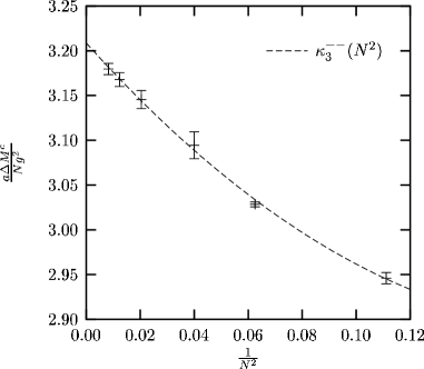
(b) 3rd eigenvalue

(c) 4th eigenvalue

(d) 5th eigenvalue

Figure 7.16: Continuum limit $0^{--}$ SU($N$) massgaps in units of $Ng^{2}/a$ as functions of $1/N^{2}$. The dashed lines are fits given in Eq. (7.38).

Figure 7.17: The lowest lying 2+1 dimensional $2^{--}$ SU($N$) massgaps in units of $Ng^{2}/a$ as a function of $1/g^{2}$.

Figure 7.18: The 2+1 dimensional continuum limit lowest $2^{--}$ SU($N$) glueball mass in units of $Ng^{2}/a$ as a function of $1/N^{2}$. The dashed line is the fit to the quadratic model of Eq. (7.40).

(a) 2nd eigenvalue

(b) 3rd eigenvalue

(c) 4th eigenvalue

(d) 5th eigenvalue

Figure 7.19: The 2+1 dimensional continuum limit $2^{--}$ SU($N$) massgaps in units of $Ng^{2}/a$ as functions of $1/N^{2}$. The dashed lines are fits given in Eq. (7.40).

Figure 7.20: An estimate of the continuum limit mass spectrum for $0^{++}$ SU($N$) glueballs in units of $Ng^{2}/a$ as a function of $1/N^{2}$. The lines are fits to the models of Eq. (7.35).

Figure 7.21: An estimate of the continuum limit mass spectrum for $0^{--}$ SU($N$) glueballs in units of $Ng^{2}/a$ as a function of $1/N^{2}$. The lines are fits to the models of Eq. (7.38).

Figure 7.22: An estimate of the continuum limit mass spectrum for $2^{--}$ SU($N$) glueballs in units of $Ng^{2}/a$ as a function of $1/N^{2}$. The lines are fits to the models of Eq. (7.40).

7.4.5 An Empirical Observation

In this subsection we present an empirical observation that could possibly be useful in the construction of simple glueball models. Since Lucini and Teper include many small area Wilson loops in their construction of excited states, we assume that they calculate the lowest few glueball states without omission. We assume the calculations presented here give higher mass glueball states. Presumably, the correct enumeration of these states is not possible without the inclusion of nonrectangular states in the minimisation basis. For example, the third lowest mass state in a given sector calculated here could be the true seventh lowest mass state. However, when our results are combined with those of Lucini and Teper an interesting empirical observation can be made. We can choose a labelling of the $0^{++}$, $0^{--}$ and $2^{--}$ excited states such that the large $N$ limit of their masses lie on a straight line as shown in Fig. 7.23. We have included the results of Lucini and Teper for $0^{--}$, $0^{--*}$, $2^{--}$ and $2^{--*}$ which do not correspond to any of the states calculated here. The straight lines are fits to the model,

$$m_{n}(J^{PC})=\gamma_{1}(2n+\gamma_{2})$$ (7.42)

where $\gamma_{1}$ and $\gamma_{2}$ are parameters and $\gamma_{2}$ is restricted to integer values. For the $J^{PC}$ states considered we obtain the following best fit models

$$m_{n}(0^{++}) = (0.256\pm 0.002)(2n+1)$$

$$m_{n}(0^{--}) = (0.151\pm 0.002)(2n+5)$$

$$m_{n}(2^{--}) = (0.1495\pm 0.0008)(2n+7).$$ (7.43)

Here $n\geq 1$ labels the $n$-th lowest mass state. We note that the fit improves in accuracy as $n$ is increased. It is interesting to note that the slopes of the $0^{--}$ and $2^{--}$ models are consistent suggesting that the constant of proportionality does not depend on $J$. Another interesting observation can be made by recasting the models in the form

$$m_{n}(0^{++}) = (0.256\pm 0.002)(2n+0+1)$$

$$m_{n}(0^{--}) = (0.151\pm 0.002)(2n+4+1)$$

$$m_{n}(2^{--}) = (0.1495\pm 0.0008)(2n+6+1).$$ (7.44)

We notice a similarity with the two dimensional harmonic oscillator spectrum,

$$E_{n}\propto 2n+J+1,$$ (7.45)

when we take into consideration the ambiguity modulo 4 of spin identification on the lattice. With this in mind we propose a simple model for the $J^{PC}$ spectrum

$$m_{n}(J^{PC})=\zeta_{PC}\left[2n+\gamma(J^{PC})+1\right],$$ (7.46)

where $\zeta_{PC}$ is a spin independent parameter and $\gamma(J^{PC})$ is an integer for which $\gamma(J^{PC})=J\,{\rm mod}\,4$. From Eq. (7.43) we have $\zeta_{--}\approx 0.15$ and $\zeta_{++}=0.256\pm 0.002$. To check this simple model we can attempt to predict the lowest lying states obtained by Lucini and Teper in the sectors that have not been considered in this chapter. We start with the $2^{++}$ sector in which Teper and Lucini obtain $1.359(12)$ and $1.822(62)$ for the $N\rightarrow\infty$ limit of the $2^{++}$ and $2^{++*}$ glueball masses in units of $Ng^{2}/a$. The predictions of Eq. (7.46), with $\gamma(2^{++})=2$ and $\zeta_{++}=0.256$, are 1.28 and 1.79 for the 1st and 2nd lowest glueball masses in units of $Ng^{2}/a$. As we would expect the prediction is better for the higher mass state. We can also consider the $1^{++}$ sector which has an equivalent spectrum to $1^{-+}$ due to the phenomenon of parity doubling Teper (1999). Lucini and Teper obtain $1.98(8)$ for the mass of the $1^{++}$ glueball in units of $Ng^{2}/a$. The model of Eq. (7.46), with $\gamma(1^{++})=5$ and $\zeta_{++}=0.256$, gives 2.048. In the $1^{--}$ sector the agreement is not as good, with Lucini and Teper obtaining $1.85(13)$ for the mass of the $1^{--}$ glueball and the model of Eq. (7.46), with $\gamma(1^{--})=9$ and $\zeta_{--}=0.15$, giving 1.812.

It will be interesting to see if the model suggested here stands up to further calculations with an extended minimisation basis and in other $J^{PC}$ sectors. The analytic techniques presented here are at a great advantage to the standard Monte Carlo techniques of Lagrangian LGT for the purpose of testing glueball models. High order excited states are readily accessible; in a variational calculation with $s$ states in the minimisation basis, $s$ glueball states are accessible. This is in contrast to competing Lagrangian calculations in which only $3$ states are currently accessible in some $J^{PC}$ sectors.

Figure 7.23: A choice of enumeration of glueball masses and the fits of Eq. (7.44).

7.4.6 Discussion

In this section we have calculated variational mass spectra for pure SU($N$) gauge theory with a simple basis of rectangular states in 2+1 dimensions. Such a basis is easy to work with computationally and is therefore a good starting point. However to accurately explore the pure gauge mass spectra additional states need to be included. Perhaps a more suitable basis would be the set of all states with an area less than some maximum value which would define the order of the calculation. The next stage beyond this would be to include higher representation states in the form of Wilson loops in which some links are covered more than once. In this way multiple glueball states could presumably be explored. The inclusion of additional small area states in the basis, in particular states which are not symmetric about reflections in coordinate axes, would also allow the calculation of spin $1$ glueball masses and also massgaps in the $P=-C$ sector.

It is important to point out that the inclusion of additional states in our minimisation basis does not present a significant challenge. The only complication would be in counting the possible overlaps of particular states. While more difficult than the counting required here, the process could presumably be automated using symbolic programming and techniques from graph theory. The analytic techniques used here would still be applicable until higher representation states were included in the minimisation basis. At that stage further character integrals would be required to handle the additional integrals arising in the calculation.

A final extension of the method presented here would be to make use of an improved ground state; a ground state which includes additional Wilson loops in the exponent. However, the advantage of using analytic techniques would then be lost, unless new technology was developed for tackling the resulting integrals. One would need to calculate the required matrix elements via Monte Carlo simulation on small lattices, losing the advantage of working on an infinite lattice with analytic expressions that we have here.

7.5 Conclusion

In this chapter we have applied the analytic techniques developed in Chapter 5, in a study of the large $N$ glueball mass spectrum in 2+1 dimensions.

A direct attempt at calculating asymptotic expansions of the generating functions was carried out in Section 7.3. While some low order large $N$ expansions were obtained, many terms appear to be needed for a direct $N\rightarrow\infty$ calculation of the matrix elements appearing in glueball mass calculations at small couplings.

Having tried a direct approach to calculating matrix elements in the $N\rightarrow\infty$ limit without success, an extrapolation technique was used. In Section 7.4 we calculated glueball masses at finite $N$, with $N$ as large as 25 in some cases. This allowed accurate $N\rightarrow\infty$ extrapolations to be made. Evidence of leading order $1/N^{2}$ finite $N$ corrections to the glueball masses was obtained, confirming a specific prediction of large $N$ gauge theory. The interpretation of the possible scaling regions was discussed and agreement with the Lagrangian study of Lucini and Teper Lucini and Teper (2002) was obtained in some cases in the $N\rightarrow\infty$ limit. The discrepancies are attributable to our use of only rectangular states in the minimisation basis. Without the inclusion of small area, nonrectangular states, it is likely that some low energy states are inaccessible. Further work will fill in the incomplete spectra presented here. Interesting empirical observations were made when the results presented here were combined with those of Lucini and Teper; the enumeration of excited states can be chosen so that the glueball mass spectrum has the structure of a two dimensional harmonic oscillator. To develop this observation into a model would require a more complete calculation of the mass spectrum with nonrectangular states in the minimisation basis and possibly a more complicated vacuum trial state.

Clearly much work remains to be done before an accurate picture of the 2+1 dimensional pure SU($N$) gauge theory spectrum is achieved within a Hamiltonian variational approach. We have demonstrated however that the analytic techniques of Hamiltonian LGT can be used for massgap calculations with $N$ as large as 25 on a desktop computer. This is significantly closer to the $N\rightarrow\infty$ limit than is currently possible with the Lagrangian approach using supercomputers. The inclusion of additional states in the minimisation basis, while not presenting a major challenge, will allow a thorough study of the 2+1 dimensional pure SU($N$) mass spectrum at least up to $N=25$.

In the next chapter we consider the extension of the analytic techniques used with success in 2+1 dimensions here, to the physically interesting case of 3+1 dimensions.

Chapter 8 3+1 Dimensions

8.1 Outline

In this chapter we explore the viability of extending the analytic techniques used with success in Chapters 6 and 7 to the calculation of glueball masses in the pure gauge sector in 3+1 dimensions. The primary difficulty lies in the calculation of expectation values in 3+1 dimensions. In Section 8.2 we briefly review what has been achieved in Hamiltonian LGT in 3+1 dimensions. We discuss the difficulties faced in 3+1 dimensions and possible solutions in Section 8.3. In Section 8.4 we consider the problem of Gauss’ law constraints. This is a topic that has been discussed in the context of Hamiltonian LGT most recently by Ligterink, Walet and Bishop Ligterink et al. (2000) and concerns the constraint equations that appear when non-abelian gauge theories are canonically quantised. In Section 8.5 we move on to the calculation of variational glueball masses on a single cube using the analytic variational technique discussed in Chapters 6 and 7. We finish in Section 8.6 with a discussion of the viability of pursuing analytic techniques for pure SU($N$) LGT in 3+1 dimensions based on the results of Section 8.5.

8.2 Introduction

From a renormalisation point of view the key difference between 2+1 and 3+1 dimensional gauge theory lies in the units of the coupling constant. As was seen in Chapter 3, 2+1 dimensional gauge theory has a coupling constant, $e^{2}$, with the dimensions of mass and so the coupling constant explicitly sets a mass scale for calculations on the lattice. In contrast the 3+1 dimensional coupling constant is dimensionless. This makes the extraction of continuum physics from lattice calculations more subtle in 3+1 dimensions than in 2+1, as discussed in Section 2.6.

On a practical level, in Hamiltonian calculations there is a more serious problem faced in moving from 2+1 to 3+1 dimensions. The analytic techniques that we have used with success in Chapters 6 and 7 are no longer applicable. These techniques rely heavily upon the fact that in 2+1 dimensions a change of variables from links to plaquettes has unit Jacobian. The form for the equivalent Jacobian in 3+1 dimensions is considerably more complicated. The most comprehensive study of the change of variables from links to plaquettes is due to Batrouni Batrouni (1982a, 1983). We discuss this change of variables in more detail in Section 8.3.

The extension of the techniques used in Chapters 6 and 7 to 3+1 dimensions is not straightforward. There are a number of immediate problems. Firstly, since plaquettes are not independent variables in 3+1 dimensions one can not automatically work in the infinite volume limit. In a precise study one would need to calculate identical quantities on different sized lattices and extrapolate to the infinite volume limit. Secondly, in the context of analytic calculations, even on small lattices the integrals involved in the calculation of basic matrix elements are considerably more complicated than those encountered in 2+1 dimensions. Such matrix elements could in principle be carried out analytically on small lattices but since the number of integration variables increases quickly with the volume of the lattice a calculation on even a $5^{3}$ lattice would seem exceedingly difficult. How quickly the infinite volume limit is reached will therefore determine the worth of pursuing analytic Hamiltonian methods in 3+1 dimensions. Finally, there is the complication of Gauss’ law which we discuss in Section 8.4.

The only Hamiltonian techniques to have been applied with any success to the case of SU(3) gauge theory in 3+1 dimensions have been strong coupling expansions, the $t$-expansion and exponential wave function methods. Each of which we now summarise.

Strong coupling perturbative techniques were used in the early days of LGT in an attempt to bridge the gap between the strong and weak coupling limits. Strong coupling expansions of the Callan-Symanzik $\beta$ function were calculated to ${\cal O}(g^{-24})$ Kogut et al. (1979); Kogut (1980) and showed signs of interpolating smoothly between the strong and weak coupling limits. This suggested that the $\beta$ function was a smooth function of the coupling with its only zero at $g=0$, providing a strong argument at the time for the continuum limit of LGT confining quarks. Corresponding strong coupling expressions for glueball masses did not share the same success. Despite strong coupling calculations to ${\cal O}(g^{-28})$ Hamer (1989) scaling was not observed in $0^{++}$, $1^{+-}$ or $2^{++}$ glueball masses.

The $t$-expansion was introduced by Horn and Weinstein Horn and Weinstein (1984) as an analytic method suitable for the study of LGT in the Hamiltonian formulation. It has been applied in the calculation of glueball masses in 3+1 dimensions for SU(2) Horn et al. (1985) and SU(3) van den Doel and Horn (1986, 1987); Horn and Lana (1991) LGT in the pure gauge sector. More recently it has been used in an attempt to calculate the lowest hadron masses Horn and Schreiber (1993). For each case, however, asymptotic scaling of masses was not directly observed. Extrapolation techniques such as Padé approximants were required to probe the weak coupling region. The extrapolated values mass ratio results agreed with Monte Carlo estimates of the time.

The coupled cluster method and related exponential wave function techniques have received by far the most attention in Hamiltonian LGT in recent years. Essentially these techniques aim to solve the Kogut-Susskind eigenvalue equation by making a suitable ansatz for the wave function. The coupled cluster method was originally constructed with applications in nuclear physics in mind Coester (1958); Coester and Kümmel (1960) but has since found the majority of its applications in molecular physics Bishop and Kümmel (1987). Its application in the context of Hamiltonian LGT is described in Refs. Schütte et al. (1997) and McKellar et al. (2000). The truncated eigenvalue method, developed by Guo, Chen and Li Guo et al. (1994), is another exponential wave function technique to have found application in Hamiltonian LGT.

A number of groups have made considerable progress in the application of exponential wave function techniques to Hamiltonian LGT in 3+1 dimensions. While most studies have explored gauge groups other than SU(3) in less than three dimensions, studies of SU(3) glueballs in 3+1 dimensions have commenced. Results tangent to the expected scaling form, indicating an approach to scaling, have been obtained for SU(3) pure gauge theory in a coupled cluster calculation by Leonard Leonard (2001). However convergence with increasing orders appears to be slow. Finite order truncation errors appear to be under more control in the truncated eigenvalue method. The first calculations of 3+1 dimensional SU(3) glueball masses with this method Hu et al. (1997) gave a $1^{+-}$ to $0^{++}$ mass ratio that was consistent with the Monte Carlo results of the time. The agreement was not as good for the $0^{--}$ to $0^{++}$ mass ratio. A convincing demonstration of asymptotic scaling has not yet been produced in a calculation of glueball masses for SU(3) in 3+1 dimensions.

More promising 3+1 dimensional results have been obtained for higher dimensional gauge groups. Ironically these results have been obtained with much simpler methods than either of the exponential wave function methods described above. Asymptotic scaling of the lowest $0^{++}$ glueball mass has been demonstrated by Chin, Long and Robson in a variational calculation on a small volume ($6^{3}$ sites) lattice for SU(5) and SU(6) Chin et al. (1986). This calculation follows the variational technique described in Chapter 6 but uses Monte Carlo rather than analytic techniques to calculate the required expectation values. It uses only plaquette states in the minimisation basis rather than the large basis of rectangular states used in Chapters 6 and 7. Naively one would hope that the same method could be explored on similar sized lattices for larger $N$, with additional states in the minimisation basis, using the analytic techniques of Chapters 6 and 7. We take this as our motivation for the studies presented in this chapter. It will become clear however that attempting a similar calculation to Chin, Long and Robson on a single cube using analytic techniques presents a significant challenge.

8.3 The Move to 3+1 Dimensions

In LGT one usually works in 2+1 dimensions to test a technique with the intention of later extending it to the physically relevant 3+1 dimensions. This may be justified in the Lagrangian approach where the time coordinate is treated on the same footing as the spatial coordinates and adding another dimension equates to nothing more than an increased load on computer memory. However, in Hamiltonian LGT two serious technical differences exists between 2+1 and 3+1 dimensions. The first is Gauss’ law and the second is related to constructing a Jacobian for transforming from link to plaquette variables.

To understand the first difference one needs to recall that Hamiltonian LGT is formulated in the temporal gauge which sets $A_{0}=0$. If one starts with the Yang-Mills Lagrangian and performs the standard equal-time quantisation, one runs into problems because the time derivative of $A_{0}$ does not appear in the Lagrangian. The variational principle gives equations of motion for the space-like components resulting in the standard Yang-Mills Hamiltonian. For the time-like component we obtain a set of algebraic constraint equations which are the analogue of Gauss’ law. There is one constraint equation for each colour component of $A_{0}$, $N^{2}-1$ for SU($N$), at each lattice site. As has been pointed out in the context of Hamiltonian LGT by Ligterink, Walet and Bishop Ligterink et al. (2000), it is only when one works with a set of variables whose number of degrees of freedom matches the number of unconstrained degrees of freedom in the theory, that one can avoid the technicalities of constraint equations. For this reason, in 2+1 dimensions we really are quite lucky. The number of plaquette variables on a square two dimensional lattice is precisely equal to the number of unconstrained variables Ligterink et al. (2000). For a three dimensional cubic lattice this is not the case. One could envisage constructing a polyhedral lattice in $d$ dimensions such that the number of faces (plaquettes) would equal the number of unconstrained variables. However such lattices appear to be prohibited by Euler’s equation which relates the number of vertices, edges and faces of polyhedra.

The other serious technical difference between 2+1 and 3+1 dimensions, that of constructing a Jacobian for transforming from link to plaquette variables, is relevant to both the Hamiltonian and Lagrangian formulations of LGT. It only becomes important when the method of choice relies on plaquette variables for its implementation. The transformation from link variables to plaquette variables is required in the approach taken in Chapters 6 and 7 to make use of the analytic results available for certain group integrals. Such a transformation does not need to be made if one is happy to use Monte Carlo techniques to handle the integrals as is the case in Ref. Chin et al. (1986).

The most complete treatment of the transformation from link to plaquette variables is due to Batrouni Batrouni (1983, 1982a) who worked in the Lagrangian formulation. His approach was based on the continuum work of Halpern Halpern (1979) who constructed a field-strength formulation of gauge theory. In Halpern’s construction the definition of the field strength $F_{\mu\nu}$ is inverted to give an expression for $A_{\mu}$ as a function of the field strength. To do this requires the choice of a suitable gauge. The Jacobian of the transformation is precisely the Bianchi identity; a constraint equation on $F_{\mu\nu}$. For the Abelian case the Bianchi identity is equivalent to the requirement that the total magnetic flux leaving a volume is zero. Batrouni developed an equivalent field strength formulation on the lattice. On the lattice, the link operators, $U_{l}$, correspond to the vector potentials, $A_{\mu}$, and the plaquette variables correspond to the field strengths, $F_{\mu\nu}$. Batrouni demonstrated that the Jacobian of the transformation from link variables to plaquette variables was the lattice analogue of the Bianchi identity. For Abelian gauge theories the lattice Bianchi identity can be separated into factors which depend only on the plaquette variables of elementary cubes, with one factor for each cube of the lattice. For non-abelian theories the Bianchi identity has only been found to separate in this way for special types of lattices, the largest volume example being an infinite tower of cubes. For the infinite lattice the Bianchi identity is a complicated nonlinear inseparable function of distant plaquette variables. Interestingly it is the only source of correlations between plaquette variables in LGT. Mean plaquette methods have been developed to deal with the added complications of the non-abelian Bianchi identity but have not progressed far Batrouni (1982b).

To summarise, Hamiltonian LGT in 3+1 dimensions faces some serious problems. Care must be taken in choosing appropriate variables to work with if constraints on the lattice electric fields are to be avoided. Additionally, if one wishes to use analytic techniques to calculate matrix elements the complications of the Bianchi identity restricts the calculations to small lattices.

8.4 Constraint Equations

In this section we focus on one of the problems faced in moving from 2+1 to 3+1 dimensions, that of Gauss’ law. From the discussion of Section 8.3 it would seem that one needs either to construct an appropriate set of variables with precisely the correct number of unconstrained degrees of freedom or be faced with the problem of building constraint equations on the lattice electric fields. As has been pointed out by Ligterink, Walet and Bishop Ligterink et al. (2000) there is an alternative. The problem of satisfying Gauss’ law can be solved by working with wave functions that are annihilated by the generator of Gauss’ law. We discuss this matter in that which follows.

In the Hamiltonian formulation of LGT we work in the temporal gauge which sets $A_{0}=0$. In terms of link variables this is equivalent to setting all time-like links to the identity. This however is only a partial gauge fixing; setting $A_{0}=0$ does not completely eliminate the arbitrariness in the definition of the vector potential, it merely reduces the set of possible gauge transformations to purely space-like ones. To see this we revert to continuum gauge theory.

In the continuum one encounters difficulties when attempting to canonically quantise SU($N$) pure gauge theory Fadeev and Slavnov (1980); Jackiw (1997). The difficulties stem from the fact that it is impossible to define a momentum conjugate to the time-like component of the vector potential $A_{0}$. This follows from the non-appearance of $\partial_{0}A^{a}_{0}$ in the Yang-Mills Lagrangian. The simplest way around the problem is to fix to the temporal gauge $A_{0}=0$ before quantising. The result is a Hamiltonian whose equations of motion do not mirror those of the Lagrangian; the non-abelian generalisation of Gauss’ Law,

$$D_{j}F^{j0}=\nabla\cdot\mbox{\boldmath$E$}=0,$$ (8.1)

is absent. One does not need to impose Gauss’ law as a constraint on the electric fields, $E^{i}=F^{i0}$. Defining $G=\nabla\cdot\mbox{\boldmath$E$}$, with the usual canonical commutation relations, it can be shown that $G^{a}$ commutes with the Hamiltonian. Consequently if one chooses to work with states $|\psi\rangle$ such that

$$G^{a}|\psi\rangle=0,$$ (8.2)

then one recovers Gauss’ law ensuring that the physics of the Lagrangian formulation is recovered.

On the lattice a similar problem arises Ligterink et al. (2000). One must therefore ensure that any state used is annihilated by the generator of Gauss’ law, in order to recover physical results with certainty. The generator of Gauss’ law on the lattice can be written as  Kogut and Susskind (1975); Kogut (1980),

$${\cal G}^{a}(\mbox{\boldmath$x$})=\sum_{i}\left[{\cal E}^{a}_{i}(\mbox{\boldmath$x$})+{\cal E}^{a}_{-i}(\mbox{\boldmath$x$})\right].$$ (8.3)

In this notation the lattice electric fields satisfy the commutation relations Kogut (1980)

$$\left[{\cal E}_{i}^{a}(\mbox{\boldmath$x$}),U_{j}(\mbox{\boldmath$y$})\right] = \lambda^{a}U_{j}(\mbox{\boldmath$y$})\delta_{ij}\delta_{\mbox{\boldmath${\scriptstyle x}$}\mbox{\boldmath${\scriptstyle y}$}}$$ (8.4)

$$\left[{\cal E}_{-i}^{a}(\mbox{\boldmath$x$}+\hat{\mbox{\boldmath$i$}}a),U_{j}(\mbox{\boldmath$y$})\right] = -U_{j}(\mbox{\boldmath$y$})\lambda^{a}\delta_{ij}\delta_{\mbox{\boldmath${\scriptstyle x}$}\mbox{\boldmath${\scriptstyle y}$}}.$$ (8.5)

It should be pointed out that in this notation we have $U^{\dagger}_{i}(\mbox{\boldmath$x$})=U_{-i}(\mbox{\boldmath$x$}+\hat{\mbox{\boldmath$i$}}a)$. For physical states we must therefore have ${\cal G}^{a}(\mbox{\boldmath$x$})|\psi\rangle=0$ for each lattice site, $x$, and all $a=1,\ldots,N^{2}-1$. It should be checked that this is the case for the one-plaquette exponential trial state. Consider first a state consisting of a single plaquette acting on the strong coupling vacuum,

$$|p_{ij}(\mbox{\boldmath$x$})\rangle={\rm Tr}\left[U_{i}(\mbox{\boldmath$x$})U_{j}(\mbox{\boldmath$x$}+\hat{\mbox{\boldmath$i$}}a)U_{-i}(\mbox{\boldmath$x$}+\hat{\mbox{\boldmath$j$}}a)U_{-j}(\mbox{\boldmath$x$})\right]|0\rangle.$$ (8.6)

Since $|0\rangle$ is annihilated by the electric field, using Eqs. (8.4) and (8.5) we immediately have

$${\cal G}^{a}(\mbox{\boldmath$y$})|p_{ij}(\mbox{\boldmath$x$})\rangle=0,$$ (8.7)

for all lattice sites, $y$, not lying on the corners of the plaquette, $p_{ij}(\mbox{\boldmath$x$})$. Consider now sites lying on the corners of the plaquette in question. In particular consider $\mbox{\boldmath$y$}=\mbox{\boldmath$x$}$. Making use of the commutation relations of Eqs. (8.4) and (8.5),

$${\cal G}^{a}(\mbox{\boldmath$x$})|p_{ij}(\mbox{\boldmath$x$})\rangle = {\rm Tr}\left[\lambda^{a}U_{i}(\mbox{\boldmath$x$})U_{j}(\mbox{\boldmath$x$}+\hat{\mbox{\boldmath$i$}}a)U_{-i}(\mbox{\boldmath$x$}+\hat{\mbox{\boldmath$j$}}a)U_{-j}(\mbox{\boldmath$x$})\right]|0\rangle$$ (8.8)

$$-{\rm Tr}\left[U_{i}(\mbox{\boldmath$x$})U_{j}(\mbox{\boldmath$x$}+\hat{\mbox{\boldmath$i$}}a)U_{-i}(\mbox{\boldmath$x$}+\hat{\mbox{\boldmath$j$}}a)U_{-j}(\mbox{\boldmath$x$})\lambda^{a}\right]|0\rangle$$

$$= 0.$$

The same applies for other sites on the plaquette. This argument is not specific to plaquettes. Gauss’ law is found to be satisfied locally by any closed Wilson loop on the lattice, traced over colour indices, acting on the strong coupling vacuum. It is easy to extend this result to products of such loops acting on $|0\rangle$. To see this we consider how Gauss’ law applies to the product of two plaquettes

$$|p_{ij}(\mbox{\boldmath$x$})p_{ij}(\mbox{\boldmath$x$}+a\hat{\mbox{\boldmath$i$}})\rangle = p_{ij}(\mbox{\boldmath$x$})p_{ij}(\mbox{\boldmath$x$}+a\hat{\mbox{\boldmath$i$}})|0\rangle.$$ (8.9)

Only at the sites $\mbox{\boldmath$x$}+a\hat{\mbox{\boldmath$i$}}$ and $\mbox{\boldmath$x$}+a(\hat{\mbox{\boldmath$i$}}+\hat{\mbox{\boldmath$j$}})$ does this case differ from the single plaquette example . Let us consider Gauss’ law at $\mbox{\boldmath$x$}_{+}=\mbox{\boldmath$x$}+a\hat{\mbox{\boldmath$i$}}$. Once again, using the fact that the lattice electric field annihilates the strong coupling vacuum, and Eqs. (8.4) and (8.5) we have

$${\cal G}^{a}(\mbox{\boldmath$x$}_{+})|p_{ij}(\mbox{\boldmath$x$})p_{ij}(\mbox{\boldmath$x$}_{+})\rangle = \sum_{k}\left[{\cal E}^{a}_{k}(\mbox{\boldmath$x$}_{+})+{\cal E}^{a}_{-k}(\mbox{\boldmath$x$}_{+}),p_{ij}(\mbox{\boldmath$x$})p_{ij}(\mbox{\boldmath$x$}_{+})\right]|0\rangle$$ (8.10)

$$= \sum_{k}\left\{\left[{\cal E}^{a}_{k}(\mbox{\boldmath$x$}_{+})+{\cal E}^{a}_{-k}(\mbox{\boldmath$x$}_{+}),p_{ij}(\mbox{\boldmath$x$})\right]p_{ij}(\mbox{\boldmath$x$}_{+})|0\rangle\right.$$

$$\left.+p_{ij}(\mbox{\boldmath$x$})\left[{\cal E}^{a}_{k}(\mbox{\boldmath$x$}_{+})+{\cal E}^{a}_{-k}(\mbox{\boldmath$x$}_{+}),p_{ij}(\mbox{\boldmath$x$}_{+})\right]|0\rangle\right\}$$

$$= 0.$$

This result is easily extended to arbitrary products of closed Wilson loops, traced over colour indices, acting on $|0\rangle$. Consequently, any function of such loops acting on $|0\rangle$ also satisfies Gauss’ law provided it admits a Taylor series expansion. The one plaquette trial state thus obeys Gauss’ law and is therefore suitable for use in simulating physical states.

8.5 The One Cube Universe

In this section we adapt the analytic techniques used with success in Chapters 6 and 7 for use in 3+1 dimensions. As a starting point we consider the case of a single cube. This will serve as a test case to assess the feasibility of a larger volume study. Our aim is to use a small basis of states to calculate 3+1 dimensional SU($N$) glueball masses variationally, and check if an approach to the correct scaling form is observed. We do not expect to achieve scaling with such a small lattice. However, an approach to scaling would warrant an extended study on larger lattices. We start with a general description of the approach. The starting point is the choice of trial state. As in 2+1 dimensions we choose to work with the one-plaquette trial state of Eq. (4.23), with the variational parameter again being fixed by minimising the vacuum energy density of Eq. (6.5). In 3+1 dimensions however the expression for the plaquette expectation value in terms of the variational parameter is significantly more complicated than for the case of 2+1 dimensions. Having fixed the variational parameter we then construct a small basis of states, with each state fitting on a single cube, and minimise the glueball mass over this basis. The process of minimising the massgap follows precisely Chapter 6. The key difficulty of working in 3+1 dimensions is the calculation of the required integrals. In the next section we explain how an analytic approximation to these integrals can be obtained.

8.5.1 SU($N$) Integrals in 3+1 Dimensions

The analytic techniques used in Chapter 6 rely on the fact that the transformation from link to plaquette variables has unit Jacobian in 2+1 dimensions. Batrouni has calculated the Jacobian for arbitrary numbers of dimensions Batrouni (1982a, 1983). For a lattice consisting of a single cube, the result of Ref. Batrouni (1982a) is

$$J = \delta(P_{1}P_{2}P_{3}P_{4}P_{5}P_{6}-1)$$ (8.11)

$$= \sum_{r}\frac{1}{d_{r}^{4}}\prod_{i=1}^{6}\chi_{r}(P_{i}),$$

where $P_{1},\ldots,P_{6}$ are the six plaquette variables on the single cube and the sum is over all characters $\chi_{r}$ of SU($N$). The second line is simply a character expansion of the first line. In the variational study of glueball masses, we need to calculate the integrals of overlapping trace variables on a single cube. It is always possible to reduce these integrals to integrals involving non-overlapping trace variables using the orthogonality properties of the characters. For example, consider the expectation value, on a single cube, of a twice covered bent rectangle, with respect to the one-plaquette trial state of Eq. (4.23),

$$\langle\phi_{0}|\begin{array}[]{c}\includegraphics[width=32.00934pt]{1.eps}\end{array}|\phi_{0}\rangle = \sum_{r}\frac{1}{d_{r}^{4}}\int\prod_{i=1}^{4}dP_{i}\chi_{r}(P_{i})e^{c{\rm Tr}(P_{i}+P^{\dagger}_{i})}$$ (8.14)

$$\times\int dP_{5}dP_{6}\chi_{r}(P_{5})\chi_{r}(P_{6})\left[\chi_{2}(P_{5}P_{6})+\chi_{11}(P_{5}P_{6})\right]e^{c{\rm Tr}(P_{5}+P_{6}+P^{\dagger}_{5}+P^{\dagger}_{6})}.$$

To proceed with this integral we need to perform character expansions. The orthogonality of the characters can then be used to write characters over two plaquettes in terms of one-plaquette characters. To demonstrate how this is done we consider the character expansion of one of the integrals in Eq. (8.14),

$$\int dP\chi_{r}(P)\chi_{2}(PP^{\prime})e^{c{\rm Tr}(P+P^{\dagger})} = \sum_{r^{\prime}}c_{r^{\prime}}\int dP\chi_{r^{\prime}}(P)\chi_{2}(PP^{\prime}).$$ (8.15)

Here the $c_{r^{\prime}}$ are given by

$$c_{r^{\prime}} = \int dP\chi_{r^{\prime}}(P)\chi_{r}(P)e^{c{\rm Tr}(P+P^{\dagger})}.$$ (8.16)

Making use of the orthogonality of characters, given by Eq. (6.19), we obtain

$$\int dP\chi_{r}(P)\chi_{2}(PP^{\prime})e^{c{\rm Tr}(P+P^{\dagger})} = \frac{c_{2}}{d_{2}}\chi_{2}(P)\chi_{2}(PP^{\prime}).$$ (8.17)

Making use of this and proceeding similarly for the analogous integral involving $\chi_{11}(P_{5}P_{6})$, we can reduce Eq. (8.14) to

$$\langle\phi_{0}|\begin{array}[]{c}\includegraphics[width=32.00934pt]{1.eps}\end{array}|\phi_{0}\rangle = \sum_{r}\frac{1}{d_{r}^{4}}\left[\int dP\chi_{r}(P)e^{c{\rm Tr}(P+P^{\dagger})}\right]^{4}$$ (8.20)

$$\times\Bigg{\{}\frac{1}{d_{2}}\left[\int dQ\chi_{2}(Q)\chi_{r}(Q)e^{c{\rm Tr}(Q+Q^{\dagger})}\right]^{2}+\frac{1}{d_{11}}\left[\int dQ\chi_{11}(Q)\chi_{r}(Q)e^{c{\rm Tr}(Q+Q^{\dagger})}\right]^{2}\Bigg{\}}.$$

The plaquette matrix element provides a more straightforward example;

$$\langle\phi_{0}|\begin{array}[]{l}\begin{picture}(20.0,25.0)\par\put(0.0,0.0){\vector(1,0){13.0}} \put(0.0,0.0){\line(1,0){20.0}} \put(20.0,0.0){\vector(0,1){13.0}} \put(20.0,0.0){\line(0,1){20.0}} \put(20.0,20.0){\vector(-1,0){13.0}} \put(20.0,20.0){\line(-1,0){20.0}} \put(0.0,20.0){\vector(0,-1){13.0}} \put(0.0,20.0){\line(0,-1){20.0}} \par\end{picture}\end{array}|\phi_{0}\rangle=\sum_{r}\frac{1}{d_{r}^{4}}\left[\int dP\chi_{r}(P)e^{c{\rm Tr}(P+P^{\dagger})}\right]^{4}\int dQ{\rm Tr}Q\chi_{r}(Q)e^{c{\rm Tr}(Q+Q^{\dagger})}.$$ (8.21)

To proceed further we need expressions for the integrals over characters that appear in each matrix element of interest. We define these character integrals generically by

$${\cal C}_{r_{1}r_{2}\ldots r_{n}}(c) = \int dP\chi_{r_{1}}(P)\chi_{r_{2}}(P)\cdots\chi_{r_{n}}(P)e^{c{\rm Tr}(P+P^{\dagger})}.$$ (8.22)

All SU($N$) integrals encountered in the calculation of glueball masses in 3+1 dimensions can be expressed in terms of character integrals. It is possible to calculate them generally, however three points need to be considered. Firstly, if we are to use the machinery of Chapter 5, we need to know how to express a given character in terms of trace variables. Secondly, as the dimension of the gauge group increases the number of independent trace variables increases rapidly. In order to contain the number of integrals required for a given order of approximation, it is necessary to express all high order trace variables in terms of a basis of lower order ones. Finally, the collection of SU($N$) integrals presented in Chapter 5 must be extended. We now address each of these points in turn.

The problem of expressing the characters of SU($N$) in terms of trace variables was solved by Bars Bars (1980) who showed that for SU($N$),

$$\chi_{n}(U)=\sum_{k_{1},\ldots,k_{n}}\delta\left(\sum_{i=1}^{n}ik_{i}-n\right)\prod_{j=1}^{n}\frac{1}{k_{j}!j^{k_{j}}}({\rm Tr}U^{j})^{k_{j}}.$$ (8.23)

General characters can then be expressed in terms of $\chi_{n}(U)$ using standard techniques from group theory Weyl (1946),

$$\chi_{r_{1}r_{2}\cdots r_{N-1}}(U)=\det\left[\chi_{r_{j}+i-j}(U)\right]_{1\leq i,j\leq N-1}.$$ (8.24)

For a given character, Eq. (8.24) produces a multinomial of traces of different powers of $U$. However, not all of these trace variables are independent. The so called Mandelstam constraints define the relationship between dependent trace variables. For SU(2) and SU(3) we have

$$\begin{array}[]{rcll}{\rm Tr}U&=&{\rm Tr}U^{\dagger}&\forall U\in{\rm SU}(2)\quad{\rm and}\\ {\rm Tr}(U^{2})&=&({\rm Tr}U)^{2}-2{\rm Tr}(U^{\dagger})&\forall U\in{\rm SU}(3).\end{array}$$ (8.27)

Similar relations can be obtained to express all trace variables in terms of ${\rm Tr}U$ for SU(2), and for SU(3) in terms of ${\rm Tr}U$ and ${\rm Tr}U^{\dagger}$. To reduce the calculation of character integrals to a manageable size, we require expressions for high power trace variables in terms of a minimal set of lower order trace variables. To do this we proceed as follows. We start with an alternative expression of $\det U=1$, satisfied for all SU($N$) matrices $U$,

$$\varepsilon_{i_{1}i_{2}\ldots i_{N}}U_{i_{1}j_{1}}U_{i_{2}j_{2}}\cdots U_{i_{N}j_{N}}=\varepsilon_{j_{1}j_{2}\ldots j_{N}}.$$ (8.28)

Here the colour indices of the group elements have been made explicit and all repeated indices are summed over. Multiplying Levi-Civita symbols produces sums of products of delta functions, the precise form of which depends on how many pairs of indices are contracted. A standard result from differential geometry will be useful here,

$$\varepsilon_{a_{1}\ldots a_{n}}\varepsilon_{b_{1}\ldots b_{n}}=\det\left(\delta_{a_{i}b_{j}}\right)_{1\leq i,j\leq n}.$$ (8.29)

Multiplying both sides of Eq. (8.28) by $U^{\dagger}_{j_{N}j_{N+1}}$ and contracting over repeated indices gives

$$\varepsilon_{i_{1}i_{2}\ldots i_{N-1}j_{N+1}}U_{i_{1}j_{1}}U_{i_{2}j_{2}}\cdots U_{i_{N-1}j_{N-1}} = \varepsilon_{j_{1}j_{2}\ldots j_{N}}U^{\dagger}_{j_{N}j_{N+1}}$$

$$\varepsilon_{l_{1}l_{2}\ldots l_{N-1}i_{N}}\varepsilon_{i_{1}i_{2}\ldots i_{N}}U_{i_{1}j_{1}}U_{i_{2}j_{2}}\cdots U_{i_{N-1}j_{N-1}} = \varepsilon_{l_{1}l_{2}\ldots l_{N-1}i_{N}}\varepsilon_{j_{1}j_{2}\ldots j_{N}}U^{\dagger}_{j_{N}i_{N}}.$$ (8.30)

In the last line we have renamed dummy indices and multiplied both sides by a Levi-Civita symbol. Making use of Eq. (8.29) in Eq. (8.30) produces a product of delta functions on each side of the equation. By introducing appropriate combinations of delta functions and contracting over repeated indices we can construct trace identities as we please. We find that identities useful in our context are produced by the introduction of delta functions and an additional matrix, $A$, which is not necessarily an element of SU($N$), into Eq. (8.30) as follows:

$$\varepsilon_{k_{1}\cdots k_{N-1}i_{N}}\varepsilon_{i_{1}\cdots i_{N}}U_{i_{1}j_{1}}A_{j_{1}k_{1}}\prod_{m=2}^{N-1}\delta_{k_{m}j_{m}}U_{i_{m}j_{m}}$$

$$\hskip 142.26378pt=\varepsilon_{k_{1}\cdots k_{N-1}i_{N}}\varepsilon_{j_{1}\cdots j_{N}}A_{j_{1}k_{1}}U^{\dagger}_{j_{N}i_{N}}\prod_{m=2}^{N-1}\delta_{k_{m}j_{m}}.$$ (8.31)

Here we have again renamed dummy indices. Some examples of SU($N$) identities obtained from Eq. (8.31) valid for all $N\times N$ matrices $A$ are as follows:

$$-{\rm Tr}U{\rm Tr}(UA)+{\rm Tr}(U^{2}A)=-{\rm Tr}A{\rm Tr}U^{\dagger}+{\rm Tr}(U^{\dagger}A) \!\!\!\forall\!\!\! U\in{\rm SU}(3)$$

$$-({\rm Tr}U)^{2}{\rm Tr}(UA)+{\rm Tr}(UA){\rm Tr}(U^{2})+2{\rm Tr}U{\rm Tr}(U^{2}A)-2{\rm Tr}(U^{3}A)$$

$$=-2{\rm Tr}A{\rm Tr}U^{\dagger}+2{\rm Tr}(U^{\dagger}A) \!\!\!\forall\!\!\! U\in{\rm SU}(4).$$ (8.32)

We require formulae for ${\rm Tr}(U^{n})$ in terms of lower order trace variables for SU($N$). Such formulae, known commonly as Mandelstam constraints, are obtained by setting $A=U^{n-N+1}$ in Eq. (8.31). In Appendix B we list the Mandelstam constraints obtained in this way up to SU(8). We see that for SU($N$) it is possible to express all characters in terms of $N-1$ trace variables. In what follows we will choose to express the general SU($N$) characters in terms of the set of trace variables, $\{{\rm Tr}U^{\dagger},{\rm Tr}U,{\rm Tr}U^{2},\ldots,{\rm Tr}U^{N-2}\}$. It may well be possible to reduce the size of this set. This would indeed improve the efficiency of our technique. However, no effort has been made to do this at this stage.

The procedure for calculating the general character integral, ${\cal C}_{r_{1}\ldots r_{n}}(c)$, is then as follows. We first express the characters $\chi_{r_{1}},\ldots,\chi_{r_{n}}$ in terms of trace variables using Eqs. (8.23) and (8.24). We then simplify these expressions using the Mandelstam constraints of Appendix B. The final step is to perform the integrals over trace variables, which is an increasingly non-trivial task as one increases the dimension of the gauge group. For instance, the general character integral for SU($N$) involves integrals over powers of the trace variables ${\rm Tr}U^{\dagger},{\rm Tr}U,{\rm Tr}U^{2},\ldots{\rm Tr}U^{N-2}$. To proceed we need the following integral,

$${\cal T}_{q_{1}\ldots q_{k}}^{p_{1}\ldots p_{k}}(c)=\int_{{\rm SU}(N)}dU({\rm Tr}U^{q_{1}})^{p_{1}}({\rm Tr}U^{q_{2}})^{p_{2}}\cdots({\rm Tr}U^{q_{k}})^{p_{k}}e^{c{\rm Tr}(U+U^{\dagger})}.$$ (8.33)

For SU($N$), the cases of interest to us here are described by, $T_{-1,1,2,\ldots,N-2}^{p_{1},\ldots,p_{N-1}}(c)$. To calculate this integral we need to extend the work of Chapter 5 and consider the generating function,

$$G_{q_{1}\ldots q_{k}}(c,\gamma_{1},\ldots,\gamma_{k})=\int_{{\rm SU}(N)}dUe^{c{\rm Tr}(U+U^{\dagger})+\sum_{i=1}^{k}\gamma_{i}{\rm Tr}(U^{q_{i}})}.$$ (8.34)

Following the procedure of Chapter 5 we obtain,

$$G_{q_{1}\ldots q_{k}}(c,\gamma_{1},\ldots,\gamma_{k}) = \sum_{l=-\infty}^{\infty}\det\left[\lambda_{l+j-i,q_{1},\ldots,q_{k}}(c,\gamma_{1},\ldots,\gamma_{k})\right]_{1\leq i,j\leq N},$$ (8.35)

with,

$$\lambda_{m,q_{1},\ldots,q_{k}}(c,\gamma_{1},\ldots,\gamma_{k}) = \sum_{s_{1},s_{2},\ldots,s_{k}=0}^{\infty}\frac{\gamma_{1}^{s_{1}}\cdots\gamma_{k}^{s_{k}}}{s_{1}!\cdots s_{k}!}I_{m+s_{1}q_{1}+\cdots+s_{k}q_{k}}(2c).$$ (8.36)

We then obtain an expression for ${\cal T}_{q_{1}\ldots q_{k}}^{p_{1}\ldots p_{k}}(c)$ by differentiating $G_{q_{1}\ldots q_{k}}$ appropriately;

$${\cal T}^{p_{1}\ldots p_{k}}_{q_{1}\ldots q_{k}}(c) = \frac{\partial^{p_{1}+\cdots+p_{k}}}{\partial\gamma_{1}^{p_{1}}\cdots\partial\gamma_{k}^{p_{k}}}G_{q_{1}\ldots q_{k}}(c,\gamma_{1},\ldots,\gamma_{k})\Bigg{|}_{\gamma_{1}=\cdots=\gamma_{k}=0}.$$ (8.37)

8.5.2 The Variational Ground State

In this section we fix the variational ground state following the usual procedure of minimising the unimproved vacuum energy density given by Eq. (6.5) with $\kappa=0$. This equation is independent of the number of dimensions. The dimensionality of the lattice arises at the stage of calculating the plaquette expectation value.

Making use of Eq. (8.21), the variational parameter can be fixed as a function of $\beta$ for the one-cube lattice. In practice, the character sum in Eq. (8.21) and the infinite $l$-sum in Eq. (8.35) need to be truncated. We truncate the infinite $l$-sum at $\pm l_{max}$ and instead of summing over all SU($N$) characters, we sum over only those characters, $r=(r_{1},r_{2},\ldots,r_{N-1})$, with $r_{max}\geq r_{1}\geq r_{2}\geq\cdots\geq r_{N-1}$. With this truncation scheme, memory constraints restrict calculations of the variational SU($N$) ground state to $N\leq 7$, when working with $r_{max}=2$ and $l_{max}=2$ on a desktop computer.

The dependence of the variational parameter on $r_{max}$ with $l_{max}=2$ is shown for various gauge groups in Fig. 8.1. As $r_{max}$ increases the variational parameter appears to converge for each $N$ considered. Moreover the convergence appears to improve as the dimension of the gauge group is increased. With the exception of SU(3), the $r_{max}=1$ and 2 results are indistinguishable on the range $0\leq\xi\leq 0.7$, where $\xi=1/(Ng^{2})$. As this is the range of interest to us later in the chapter we restrict further calculations to $r_{max}=1$.

The SU($N$) variational parameters on the one-cube lattice with $r_{max}=1$ and $l_{max}=2$ are shown for various $N$ in Fig. 8.2. The results do not differ greatly. The corresponding variational energy densities are shown in Fig. 8.3.

Figure 8.1: The one cube SU($N$) variational parameter as a function of $\beta$ for various $N$ showing the dependence on the character sum truncation.

Figure 8.2: The one cube SU($N$) variational parameter in units of $N$ as a function of $1/(Ng^{2})$ for various $N$.

Figure 8.3: The one cube SU($N$) energy density in units of $N$ as a function of $1/g^{2}$ for various $N$.

8.5.3 Expressions for the Glueball Mass

We follow precisely the method described in Section 6.5 for the calculation of 3+1 dimensional glueball masses on a single cube. Here, however, we choose a different basis of states to minimise over. Instead of rectangular loops, we use states which fit on a single cube. We start with a basis of two states, the plaquettes and the bent rectangles,

$$B = \{|1\rangle,|2\rangle\},$$ (8.38)

with

$$|i\rangle = \sum_{\mbox{\boldmath${\scriptstyle x}$}}\left[F_{i}(x)-\langle F_{i}(x)\rangle\right]|\phi_{0}\rangle$$ (8.39)

and

$$F_{1}(x) = \begin{array}[]{c}\includegraphics[width=21.33955pt]{30.eps}\end{array}\pm\begin{array}[]{c}\includegraphics[width=21.33955pt]{31.eps}\end{array}$$ (8.42)

$$F_{2}(x) = \begin{array}[]{c}\includegraphics[width=32.00934pt]{9.eps}\end{array}\pm\begin{array}[]{c}\includegraphics[width=32.00934pt]{32.eps}\end{array}.$$ (8.45)

In 3+1 dimensions, the “+” sign corresponds to the $0^{++}$ state and the “$-$” sign corresponds to the $1^{+-}$ state Hamer (1989). In order to calculate the glueball masses, we need expressions for the matrix elements $N^{C}_{ii^{\prime}}$ and $D^{C}_{ii^{\prime}}$ of Eqs. (6.9) and (6.10) respectively. Here the superscript, $C$, denotes the charge conjugation eigenvalue, $C=\pm 1$, of the state in question. Making use of Eq. (6.20) and carefully counting the number of possible overlaps between different loops we arrive at

$$\frac{2aN^{C}_{11}}{N_{p}g^{2}} = 4\left[\Big{\langle}\Big{\langle}\!\begin{array}[]{l}\begin{picture}(20.0,25.0)\par\par\par\put(0.0,0.0){\line(4,1){16.0}} \put(4.0,4.0){\line(4,-1){16.0}} \put(16.0,4.0){\line(0,1){12.0}} \put(16.0,4.0){\vector(0,1){9.0}} \put(16.0,16.0){\line(-1,0){12.0}} \put(16.0,16.0){\vector(-1,0){9.0}} \put(4.0,16.0){\line(0,-1){12.0}} \put(4.0,16.0){\vector(0,-1){9.0}} \par\put(20.0,0.0){\vector(0,1){13.0}} \put(20.0,0.0){\line(0,1){20.0}} \put(20.0,20.0){\vector(-1,0){13.0}} \put(20.0,20.0){\line(-1,0){20.0}} \put(0.0,20.0){\vector(0,-1){13.0}} \put(0.0,20.0){\line(0,-1){20.0}} \par\end{picture}\end{array}\!\Big{\rangle}\Big{\rangle}-\frac{1}{N}\Big{\langle}\Big{\langle}\!\begin{array}[]{l}\begin{picture}(20.0,25.0)\par\par\put(0.0,0.0){\vector(1,0){13.0}} \put(0.0,0.0){\line(1,0){20.0}} \put(4.0,4.0){\vector(1,0){9.0}} \put(4.0,4.0){\line(1,0){12.0}} \par\put(16.0,4.0){\line(0,1){12.0}} \put(16.0,4.0){\vector(0,1){9.0}} \put(16.0,16.0){\line(-1,0){12.0}} \put(16.0,16.0){\vector(-1,0){9.0}} \put(4.0,16.0){\line(0,-1){12.0}} \put(4.0,16.0){\vector(0,-1){9.0}} \par\put(20.0,0.0){\vector(0,1){13.0}} \put(20.0,0.0){\line(0,1){20.0}} \put(20.0,20.0){\vector(-1,0){13.0}} \put(20.0,20.0){\line(-1,0){20.0}} \put(0.0,20.0){\vector(0,-1){13.0}} \put(0.0,20.0){\line(0,-1){20.0}} \par\end{picture}\end{array}\!\Big{\rangle}\Big{\rangle}+C\left(-N+\frac{1}{N}\Big{\langle}\Big{\langle}\!\begin{array}[]{l}\begin{picture}(20.0,25.0)\par\par\put(0.0,0.0){\vector(1,0){13.0}} \put(0.0,0.0){\line(1,0){20.0}} \put(4.0,4.0){\vector(0,1){9.0}} \put(4.0,4.0){\line(0,1){12.0}} \par\put(4.0,16.0){\line(1,0){12.0}} \put(4.0,16.0){\vector(1,0){9.0}} \put(16.0,16.0){\line(0,-1){12.0}} \put(16.0,16.0){\vector(0,-1){9.0}} \put(16.0,4.0){\line(-1,0){12.0}} \put(16.0,4.0){\vector(-1,0){9.0}} \par\put(20.0,0.0){\vector(0,1){13.0}} \put(20.0,0.0){\line(0,1){20.0}} \put(20.0,20.0){\vector(-1,0){13.0}} \put(20.0,20.0){\line(-1,0){20.0}} \put(0.0,20.0){\vector(0,-1){13.0}} \put(0.0,20.0){\line(0,-1){20.0}} \par\end{picture}\end{array}\!\Big{\rangle}\Big{\rangle}\right)\right]$$ (8.49)

$$\frac{D^{C}_{11}}{N_{p}} = 2\Big{\langle}\Big{\langle}\!\begin{array}[]{l}\begin{picture}(20.0,25.0)\par\par\put(0.0,0.0){\vector(1,0){13.0}} \put(0.0,0.0){\line(1,0){20.0}} \put(4.0,4.0){\vector(1,0){9.0}} \put(4.0,4.0){\line(1,0){12.0}} \par\put(16.0,4.0){\line(0,1){12.0}} \put(16.0,4.0){\vector(0,1){9.0}} \put(16.0,16.0){\line(-1,0){12.0}} \put(16.0,16.0){\vector(-1,0){9.0}} \put(4.0,16.0){\line(0,-1){12.0}} \put(4.0,16.0){\vector(0,-1){9.0}} \par\put(20.0,0.0){\vector(0,1){13.0}} \put(20.0,0.0){\line(0,1){20.0}} \put(20.0,20.0){\vector(-1,0){13.0}} \put(20.0,20.0){\line(-1,0){20.0}} \put(0.0,20.0){\vector(0,-1){13.0}} \put(0.0,20.0){\line(0,-1){20.0}} \par\end{picture}\end{array}+C\begin{array}[]{l}\begin{picture}(20.0,25.0)\par\par\put(0.0,0.0){\vector(1,0){13.0}} \put(0.0,0.0){\line(1,0){20.0}} \put(4.0,4.0){\vector(0,1){9.0}} \put(4.0,4.0){\line(0,1){12.0}} \par\put(4.0,16.0){\line(1,0){12.0}} \put(4.0,16.0){\vector(1,0){9.0}} \put(16.0,16.0){\line(0,-1){12.0}} \put(16.0,16.0){\vector(0,-1){9.0}} \put(16.0,4.0){\line(-1,0){12.0}} \put(16.0,4.0){\vector(-1,0){9.0}} \par\put(20.0,0.0){\vector(0,1){13.0}} \put(20.0,0.0){\line(0,1){20.0}} \put(20.0,20.0){\vector(-1,0){13.0}} \put(20.0,20.0){\line(-1,0){20.0}} \put(0.0,20.0){\vector(0,-1){13.0}} \put(0.0,20.0){\line(0,-1){20.0}} \par\end{picture}\end{array}\!\Big{\rangle}\Big{\rangle}+10\Bigg{\langle}\!\!\!\Bigg{\langle}\!\begin{array}[]{c}\includegraphics[width=32.00934pt]{21.eps}\end{array}\!\!+C\!\!\begin{array}[]{c}\includegraphics[width=32.00934pt]{21.eps}\end{array}\!\Bigg{\rangle}\!\!\!\Bigg{\rangle}-24\left(\frac{C+1}{2}\right)\Big{\langle}\Big{\langle}\!\!\begin{array}[]{l}\begin{picture}(20.0,25.0)\par\put(0.0,0.0){\vector(1,0){13.0}} \put(0.0,0.0){\line(1,0){20.0}} \put(20.0,0.0){\vector(0,1){13.0}} \put(20.0,0.0){\line(0,1){20.0}} \put(20.0,20.0){\vector(-1,0){13.0}} \put(20.0,20.0){\line(-1,0){20.0}} \put(0.0,20.0){\vector(0,-1){13.0}} \put(0.0,20.0){\line(0,-1){20.0}} \par\end{picture}\end{array}\!\!\Big{\rangle}\Big{\rangle}^{2}$$ (8.55)

$$\frac{2aN^{C}_{21}}{N_{p}g^{2}} = 12\Bigg{\langle}\!\!\!\Bigg{\langle}\!\frac{1}{N}\begin{array}[]{c}\includegraphics[width=32.00934pt]{29.eps}\end{array}-\frac{1}{N^{2}}\begin{array}[]{c}\includegraphics[width=32.00934pt]{16.eps}\end{array}+C\left(-\begin{array}[]{l}\begin{picture}(20.0,25.0)\par\put(0.0,0.0){\vector(1,0){13.0}} \put(0.0,0.0){\line(1,0){20.0}} \put(20.0,0.0){\vector(0,1){13.0}} \put(20.0,0.0){\line(0,1){20.0}} \put(20.0,20.0){\vector(-1,0){13.0}} \put(20.0,20.0){\line(-1,0){20.0}} \put(0.0,20.0){\vector(0,-1){13.0}} \put(0.0,20.0){\line(0,-1){20.0}} \par\end{picture}\end{array}+\frac{1}{N^{2}}\begin{array}[]{c}\includegraphics[width=32.00934pt]{17.eps}\end{array}\right)\!\Bigg{\rangle}\!\!\!\Bigg{\rangle}$$ (8.60)

$$\frac{D^{C}_{21}}{N_{p}} = \frac{8}{N}\Bigg{\langle}\!\!\!\Bigg{\langle}\!\begin{array}[]{c}\includegraphics[width=32.00934pt]{16.eps}\end{array}+C\begin{array}[]{c}\includegraphics[width=32.00934pt]{17.eps}\end{array}\!\Bigg{\rangle}\!\!\!\Bigg{\rangle}+\frac{16}{N}\Bigg{\langle}\!\!\!\Bigg{\langle}\!\begin{array}[]{c}\includegraphics[width=32.00934pt]{14.eps}\end{array}+C\begin{array}[]{c}\includegraphics[width=32.00934pt]{15.eps}\end{array}\!\Bigg{\rangle}\!\!\!\Bigg{\rangle}$$ (8.68)

$$-\frac{48}{N}\left(\frac{C+1}{2}\right)\Big{\langle}\Big{\langle}\!\begin{array}[]{l}\begin{picture}(20.0,25.0)\par\put(0.0,0.0){\vector(1,0){13.0}} \put(0.0,0.0){\line(1,0){20.0}} \put(20.0,0.0){\vector(0,1){13.0}} \put(20.0,0.0){\line(0,1){20.0}} \put(20.0,20.0){\vector(-1,0){13.0}} \put(20.0,20.0){\line(-1,0){20.0}} \put(0.0,20.0){\vector(0,-1){13.0}} \put(0.0,20.0){\line(0,-1){20.0}} \par\end{picture}\end{array}\!\Big{\rangle}\Big{\rangle}\Bigg{\langle}\!\!\!\Bigg{\langle}\!\begin{array}[]{c}\includegraphics[width=32.00934pt]{20.eps}\end{array}\!\Bigg{\rangle}\!\!\!\Bigg{\rangle}.$$

Here we have introduced the notation

$$\langle\!\langle O\rangle\!\rangle=\langle\phi_{0}|O|\phi_{0}\rangle.$$ (8.69)

The combinatorics which lead to the coefficients in the matrix elements in Eq. (8.68) are a result of counting the possible overlaps within a single cube. The remaining matrix elements $N_{22}$ and $D_{22}$ can be calculated similarly, resulting in

$$\frac{2aN^{C}_{22}}{N_{p}g^{2}} = 12\left[\Bigg{\langle}\!\!\!\Bigg{\langle}\!\begin{array}[]{c}\includegraphics[width=32.00934pt]{26.eps}\end{array}\!\Bigg{\rangle}\!\!\!\Bigg{\rangle}-\frac{1}{N}\Bigg{\langle}\!\!\!\Bigg{\langle}\!\begin{array}[]{c}\includegraphics[width=32.00934pt]{1.eps}\end{array}\!\Bigg{\rangle}\!\!\!\Bigg{\rangle}+C\left(-N+\frac{1}{N}\Bigg{\langle}\!\!\!\Bigg{\langle}\!\begin{array}[]{c}\includegraphics[width=32.00934pt]{2.eps}\end{array}\!\Bigg{\rangle}\!\!\!\Bigg{\rangle}\right)\right]$$ (8.78)

$$+\frac{32}{N}\Bigg{\langle}\!\!\!\Bigg{\langle}\!\frac{1}{N}\begin{array}[]{c}\includegraphics[width=32.00934pt]{45.eps}\end{array}-\frac{1}{N^{2}}\begin{array}[]{c}\includegraphics[width=32.00934pt]{18.eps}\end{array}+C\left(-\begin{array}[]{c}\includegraphics[width=32.00934pt]{35.eps}\end{array}+\frac{1}{N^{2}}\begin{array}[]{c}\includegraphics[width=32.00934pt]{19.eps}\end{array}\right)\!\Bigg{\rangle}\!\!\!\Bigg{\rangle}$$

$$\frac{D^{C}_{22}}{N_{p}} = 4\Bigg{\langle}\!\!\!\Bigg{\langle}\!\begin{array}[]{c}\includegraphics[width=32.00934pt]{1.eps}\end{array}+C\begin{array}[]{c}\includegraphics[width=32.00934pt]{2.eps}\end{array}\!\Bigg{\rangle}\!\!\!\Bigg{\rangle}+\frac{24}{N^{2}}\Bigg{\langle}\!\!\!\Bigg{\langle}\!\begin{array}[]{c}\includegraphics[width=32.00934pt]{18.eps}\end{array}+C\begin{array}[]{c}\includegraphics[width=32.00934pt]{19.eps}\end{array}\!\Bigg{\rangle}\!\!\!\Bigg{\rangle}$$ (8.87)

$$+\frac{20}{N^{2}}\Bigg{\langle}\!\!\!\Bigg{\langle}\!\begin{array}[]{c}\includegraphics[width=32.00934pt]{24.eps}\end{array}+C\begin{array}[]{c}\includegraphics[width=32.00934pt]{25.eps}\end{array}\!\Bigg{\rangle}\!\!\!\Bigg{\rangle}-\frac{96}{N^{2}}\left(\frac{C+1}{2}\right)\Bigg{\langle}\!\!\!\Bigg{\langle}\!\begin{array}[]{c}\includegraphics[width=32.00934pt]{20.eps}\end{array}\!\Bigg{\rangle}\!\!\!\Bigg{\rangle}^{2}.$$

Having calculated $N^{C}_{ii^{\prime}}$ and $D^{C}_{ii^{\prime}}$, we follow the minimisation procedure described in Chapter 6 to arrive at the glueball mass, $\Delta M^{PC}$.

8.5.4 Results

In this section we present calculations of the $0^{++}$ (symmetric) and $1^{+-}$ (antisymmetric) glueball masses on the one-cube lattice for SU($N$) with $4\leq N\leq 7$. We first define the rescaled glueball mass, $\mu^{PC}$, corresponding to $\Delta M^{PC}$ as follows:

$$\mu^{PC}=\log(a\Delta M^{PC}\xi^{-51/121})-\frac{51}{121}\log\left(\frac{48\pi^{2}}{11}\right)+\frac{24\pi^{2}}{11}\xi.$$ (8.88)

Here, as usual, $P$ and $C$ denote the parity and charge conjugation eigenvalues of the state in question. From the discussion Section 2.6 asymptotic scaling of a glueball mass is observed if the corresponding rescaled glueball mass becomes constant for some range of couplings.

The results for the rescaled symmetric glueball mass are shown in Fig. 8.4. Fig. 8.4(a) shows the rescaled glueball mass calculated with only plaquettes in the minimisation basis. Fig. 8.4(b) shows the same quantity calculated with the minimisation basis of Eq. (8.38). The aim of this exploratory study is to observe whether or not a move toward scaling is apparent as the number of states in the minimisation basis is increased. This is clearly not the case for the symmetric glueball mass on the range of couplings explored here. There is no sign of $\mu^{++}$ becoming constant on any range of couplings within $0\leq\xi\leq 0.55$.

The prospects are marginally better for the antisymmetric case. The results for the rescaled antisymmetric glueball mass are displayed in Fig. 8.5. A move toward scaling is observed, most clearly for the $N=7$ case, near $\xi=0.38$. This matches the region of couplings for which Chin, Long and Robson observed scaling of the $0^{++}$ glueball mass, for $N=5$ and 6, on a $6^{3}$ lattice using only plaquettes in their minimisation basis Chin et al. (1986).

(a) Calculated with only plaquettes in the minimisation basis

(b) Calculated with both plaquettes and bent rectangles in the minimisation basis

Figure 8.4: The one cube SU($N$) $0^{++}$ rescaled glueball mass as a function of $1/(Ng^{2})$ for various $N$ obtained with different minimisation bases.

(a) Calculated with only plaquettes in the minimisation basis

(b) Calculated with both plaquettes and bent rectangles in the minimisation basis

Figure 8.5: The one cube SU($N$) $1^{+-}$ rescaled glueball mass as a function of $1/(Ng^{2})$ for various $N$ obtained with different minimisation bases.

8.5.5 String Tension

If the exploratory study presented here was to be extended to larger lattices, at some stage it would be useful to compute the string tension, $\sigma$. It is common for calculations in Lagrangian LGT to express results for masses in units of $\sqrt{\sigma}$. This allows masses calculated on the lattice to be expressed in MeV since the string tension can be calculated in MeV from the decay of heavy quarkonia for example. In the Hamiltonian formulation, precise calculations of the string tension have only been performed in the strong coupling regime. Variational estimates, at least for SU(2) Arisue et al. (1983), have not exhibited asymptotic scaling when making use of the one-plaquette ground state of Eq. (4.23). It is possible that the situation may be improved for higher dimensional gauge groups but this has not yet been tested.

In this section we calculate the symmetric and antisymmetric glueball masses in units of $\sqrt{\sigma}$. For the string tension, since reliable variational results are not available, we use the strong coupling expansions of Kogut and Shigemitsu Kogut and Shigemitsu (1980). These are available for SU(5) and SU(6), as well as SU(2) and SU(3) which we do not consider here.

Since the square root of the string tension has units of mass, the ratio of a mass to the string tension is constant in a scaling region. Again, with the crude model presented here, we do not expect to observe scaling. We seek only an indication of an approach to scaling. Such behaviour would warrant further study.

The results for the symmetric states are shown in Fig. 8.6. Since we perform calculations with two states in the minimisation basis, the two lowest mass states are accessible. In Fig. 8.6(a) the results for the lowest mass state are shown. Calculations with different minimisation bases are shown, with the “SU$(N)$-plaquettes” label indicating that only plaquette states are used. For each case the glueball mass has a local minimum in the range $0.33\leq\xi\leq 0.37$. The various results do not differ greatly. There is no sign of improved scaling behaviour when either bent rectangles are included or $N$ is increased. The effect of including bent rectangles is to lower the local minimum.

The second lowest glueball mass is shown in Fig. 8.6(b). Again, no improvement in scaling behaviour is seen as $N$ is increased. In Fig. 8.6 the horizontal lines indicate the 3+1 dimensional SU(5) calculations (and error bars) of Lucini and Teper Lucini and Teper (2001). Interestingly, both masses calculated here with a simplistic model, have minima that lie within the error bars.

We now move on to the antisymmetric states. The results for the antisymmetric glueball masses in units of $\sqrt{\sigma}$ are shown in Fig. 8.7. The results are more promising than the symmetric case. We see an improved approach to scaling when bent rectangles are included in the minimisation basis for the lowest glueball mass. For this case the glueball mass shows promising signs of becoming constant in the ranges $0.32\leq\xi\leq 0.39$ for SU(6) and $0.3\leq\xi\leq 0.37$ for SU(5). Only marginal improvement in scaling behaviour is evident as $N$ is increased from 5 to 6. For each of these cases no data is available for comparison to our knowledge. Such promising signs are not apparent in the second lowest glueball mass in this sector, as seen in Fig. 8.7(b).

It would be interesting to perform analogous calculations for SU(7), for which the most promising results were displayed in Section 8.5.4. However strong coupling expansions for the SU(7) string tension are not available in Ref. Kogut and Shigemitsu (1980) and have not been published elsewhere to our knowledge.

(a) Lowest energy state

(b) Second lowest energy state

Figure 8.6: The one cube SU(5) and SU(6) $0^{++}$ glueball masses in units of $\sqrt{\sigma}$ as functions of $1/(Ng^{2})$. The horizontal lines indicate the result and error bars of the SU(5) $0^{++}$ calculation of Lucini and Teper Lucini and Teper (2001).

(a) Lowest energy state

(b) Second lowest energy state

Figure 8.7: The one cube SU(5) and SU(6) $1^{+-}$ glueball masses in units of $\sqrt{\sigma}$ as functions of $1/(Ng^{2})$.

8.6 Future Work

In this chapter we have studied the variational $0^{++}$ and $1^{+-}$ glueball masses on a single cube in 3+1 dimensions. Our intention was to determine the viability of using analytic Hamiltonian methods in 3+1 dimensional glueball mass calculations. With such a crude small volume approximation and a minimisation basis containing only two states, the observation of asymptotic scaling was not expected. Promising signs of an approach to asymptotic scaling were displayed by the $1^{+-}$ glueball mass, as $N$ was increased, at couplings close to the scaling window observed by a comparable, but larger volume, study by Chin, Long and Robson Chin et al. (1986). Interesting results were also observed for calculations of the glueball masses in units of the string tension. With no variational results for the string tension available, the strong coupling results of Kogut and Shigemitsu Kogut and Shigemitsu (1980) were used. Interestingly, the mass of both SU(5) $0^{++}$ glueball states calculated had minima which were consistent with the Lagrangian calculation of Lucini and Teper Lucini and Teper (2001). Better scaling behaviour was exhibited by the SU(5) and SU(6) $1^{+-}$ states, although no alternative calculations are available for comparison to our knowledge. For the lowest mass $1^{+-}$ states calculated, the scaling behaviour was improved by increasing the number of states in the minimisation basis and the dimension of the gauge group. The promising results observed in this chapter warrant further study on larger lattices, with additional states in the minimisation basis.

To extend this calculation to larger lattices and minimisation bases, two challenges will be faced. Firstly, the correct implementation of the Bianchi identity, within our plaquette based analytic approach, forces the number of integration variables to grow quickly with the volume. New approaches to handling the general character integrals may need to be developed in order to avoid the inevitable memory restrictions. Secondly, great care will need to be taken in the counting of overlaps between different states. This process could, in principle, be automated using techniques from graph theory and symbolic programming.

It would also be of interest to extend the calculation presented here to larger $N$. To do this a more efficient technique for handling the general character integrals would need to be developed to minimise the memory demands of the calculation. The following is just one possibility. It is likely, that by expressing the products of characters appearing in the character integrals as sums of characters, one could reduce the memory requirements of the calculation drastically. The general character integrals could then be expressed in terms of integrals of the form,

$$G_{r}(c) = \int_{{\rm SU}(N)}dU\chi_{r}(U^{\dagger})e^{c{\rm Tr}(U+U^{\dagger})},$$ (8.89)

where $r=(r_{1},r_{2},\ldots r_{N-1})$ labels a representation of SU($N$). Having completed the calculations presented in this chapter, it was discovered that $G_{r}(c)$ can be handled using the techniques of Chapter 5, with the result,

$$G_{r}(c) = \sum_{l=-\infty}^{\infty}\det\left[I_{r_{i}+l+j-i}(2c)\right]_{1\leq i,j\leq N}.$$ (8.90)

The final stage of this improvement would be to find a convenient way to express the products of characters appearing in the calculation as a sum of characters. This would be possible with the symbolic manipulation of Young tableaux.

Chapter 9 Conclusion

This thesis has been concerned with the study of two topics: improvement and the use of analytic techniques in Hamiltonian LGT. In this chapter we summarise our key results and discuss the directions that further work should take.

Chapters 3 and 4 were concerned primarily with the issue of improvement. In Chapter 3 a technique allowing the straightforward construction of lattice Hamiltonians was developed. Using this direct approach a number of improved Hamiltonians were derived. The key advantage of our approach is that it allows the straightforward construction of improved kinetic Hamiltonians with a finite number of terms, a task that has proved nontrivial in the past. In Chapter 4 two simple tests of improvement, a strong coupling calculation of the U(1) Callan-Symanzik $\beta$ function in 3+1 dimensions and a mean field calculation of the SU(2) lattice specific heat in 2+1 dimensions, were presented. For each example considered, the tadpole improved Hamiltonians (when they were used) achieved the greatest level of improvement followed by the classically improved Hamiltonians and then the Kogut-Susskind Hamiltonians.

In Chapter 5, techniques which allow the analytic calculation of SU($N$) matrix elements in 2+1 dimensions were developed. This chapter generalised the methods that have been employed in variational SU(2) LGT calculations for almost 20 years, to the general case of SU($N$). A close connection with the fields of random matrices and combinatorics was also discussed.

In Chapter 6, the analytic techniques of Chapter 5 were applied in the calculation of $N=2,3,4,$ and 5 glueball masses in 2+1 dimensions. Kogut-Susskind, improved and tadpole improved Hamiltonians, all of which were derived in Chapter 3, were used and their results compared. For each case considered, the lowest mass results obtained were considerably higher than the lowest glueball masses obtained by comparable Hamiltonian and Lagrangian calculations. However, the lowest mass states obtained in the $0^{++}$ and $0^{--}$ sectors were close in mass to the respective excited states, $0^{++*}$ and $0^{--**}$, of Teper and Lucini Teper (1999); Lucini and Teper (2002). In the $0^{++}$ sector this agreement improved as $N$ was increased, and for each $N$ the agreement was closer for the improved calculations. This situation was replicated in the $0^{--}$ sector if the SU(4) results were excluded. For SU(4), the lowest unimproved glueball mass was closer to the mass of Teper and Lucini’s $0^{--**}$ state than the improved results. The problem of enumerating states can be attributed to the fact that the calculations presented in Chapter 6 used a basis of rectangular states. The competing calculations incorporate additional nonrectangular states. Without the inclusion of small area, nonrectangular states in the calculation, it is possible that some low mass states are inaccessible. Further calculations, which include nonrectangular states in the minimisation basis, are needed to clarify this issue. Including such additional states will also allow spin 1 and $P=-C$ states to be studied, and permit a more complete study of the spin 0 and 2 glueball mass spectra.

In Chapter 7 we presented the first steps of a study of the SU($N$) glueball mass spectrum in the large $N$ limit using the techniques of Chapter 6. Our motivation was the Maldacena conjecture which, in its simplest form, predicts a precise correspondence between certain string theories and gauge theories in the large $N$ limit. Using analytic Hamiltonian techniques, calculations with $N$ as large as 25 were possible on a desktop computer, in contrast to comparable Lagrangian calculations which have reached $N=6$. With such large $N$ glueball masses accessible, reliable extrapolations to the $N\rightarrow\infty$ were possible. The results provided evidence for leading order $1/N^{2}$ finite $N$ corrections to the glueball masses, verifying a specific prediction of large $N$ gauge theory.

In Chapter 8 we moved on to the physically interesting case of 3+1 dimensions. There we studied the viability of adapting the analytic techniques used with success in Chapters 6 and 7 to 3+1 dimensions. A simple variational calculation of $0^{++}$ and $1^{+-}$ glueball masses was carried out on a single cube, with only two states in the minimisation basis. With such a simplistic approximation asymptotic scaling was not expected. However, it was hoped that with the use of analytic Hamiltonian techniques, large values of $N$ could be reached. This was not the case, with memory constraints restricting calculations to $N\leq 7$ on a one cube lattice. Our motivation for attempting this calculation was a variational Hamiltonian study by Chin, Long and Robson Chin et al. (1986) which demonstrated asymptotic scaling of the $0^{++}$ glueball mass on a $6^{3}$ lattice for $N=5$ and 6, with improved scaling observed as $N$ was increased. Promising signs of an approach to asymptotic scaling were observed in Chapter 8 for the $1^{+-}$ state, in the same region of couplings as scaling was seen by Chin, Long and Robson. No such signs were observed for the $0^{++}$ state. The extension to larger lattices thus seems warranted. Such extensions will be hampered by memory constraints unless new techniques for handling the general character integrals are developed. Another important improvement, which does not pose a serious problem, will be the inclusion of more states in the minimisation basis. The applicability of analytic variational techniques in 3+1 dimensions will thus be determined by how quickly the infinite volume limit is reached.

While we have derived various improved Hamiltonians and put them to use in glueball mass calculations in 2+1 dimensions, their use in 3+1 dimensional non-abelian LGT is untested. The next stages of a 3+1 dimensional calculation, within the variational analytic approach presented here, would incorporate improved Hamiltonians and move beyond a single cube. It is possible that in such a calculation the use of an improved Hamiltonian could mean the difference between observing and not observing scaling on the range of couplings available.

The results of this thesis demonstrate that the analytic techniques of Hamiltonian LGT can compete with the traditional Monte Carlo techniques of Lagrangian LGT, at least in the calculation of glueball masses in 2+1 dimensions. The use of the analytic techniques presented here are by no means restricted to variational calculations. It is possible that they will find use in coupled cluster calculations, or in the moment calculations of the plaquette expansion method Hollenberg (1993). The move to 3+1 dimensions is formidable but the calculations of Chapter 8 suggest that analytic techniques may by feasible, at least for large $N$, provided the infinite volume limit is reached quickly.

Appendix A Commutation Relations

In improved Hamiltonian LGT calculations, one encounters matrix elements of the form:

$$\langle\phi_{0}|\sum_{\boldsymbol{x},i}{\rm Tr}\left[{\cal E}_{i}(\boldsymbol{x}){\cal E}_{i}(\boldsymbol{x})\right]|\phi_{0}\rangle\quad{\rm and}\quad\langle\phi_{0}|\sum_{\boldsymbol{x},i}{\rm Tr}\left[{\cal E}_{i}(\boldsymbol{x})U_{i}(\boldsymbol{x}){\cal E}_{i}(\boldsymbol{x}+a\boldsymbol{i})U^{\dagger}_{i}(\boldsymbol{x})\right]|\phi_{0}\rangle.$$ (A.1)

The first of these is easily handled. One simply writes the electric field operators as ${\cal E}_{i}(\boldsymbol{x})={\cal E}^{\alpha}_{i}(\boldsymbol{x})\lambda^{\alpha}$ and uses the normalisation condition, Eq. (3.5), to give

$$\langle\phi_{0}|\sum_{\boldsymbol{x},i}{\rm Tr}\left[{\cal E}_{i}(\boldsymbol{x}){\cal E}_{i}(\boldsymbol{x})\right]|\phi_{0}\rangle = \frac{1}{2}\sum_{\boldsymbol{x},i}\langle\phi_{0}|{\cal E}^{\alpha}_{i}(\boldsymbol{x}){\cal E}^{\alpha}_{i}(\boldsymbol{x})|\phi_{0}\rangle.$$ (A.2)

Let the trial state, $|\phi_{0}\rangle$, have the form $|\phi_{0}\rangle=e^{S}|0\rangle$, where $S$ is a function of link variables and $S^{\dagger}=S$. Then

$$\sum_{\boldsymbol{x},i}\langle\phi_{0}|{\cal E}^{\alpha}_{i}(\boldsymbol{x}){\cal E}^{\alpha}_{i}(\boldsymbol{x})|\phi_{0}\rangle=-\sum_{\boldsymbol{x},i}\langle 0|\left[{\cal E}^{\alpha}_{i}(\boldsymbol{x}),e^{S}\right]\left[{\cal E}^{\alpha}_{i}(\boldsymbol{x}),e^{S}\right]|0\rangle.$$ (A.3)

Making use of the Baker-Hausdorff formula, Eq. (3.19), we can derive the following result,

$$e^{S}{\cal E}^{\alpha}_{i}(\boldsymbol{x})e^{-S} = {\cal E}^{\alpha}_{i}(\boldsymbol{x})-[{\cal E}^{\alpha}_{i}(\boldsymbol{x}),S]+\frac{1}{2}[[{\cal E}^{\alpha}_{i}(\boldsymbol{x}),S],S]+\ldots$$ (A.4)

$$= {\cal E}^{\alpha}_{i}(\boldsymbol{x})-[{\cal E}^{\alpha}_{i}(\boldsymbol{x}),S].$$

The last line follows from the fact that $S$ is a function of link variables and the commutation relation of Eq. (8.4). Some rearrangement of Eq. (A.4) leads to the useful result,

$$\left[{\cal E}^{\alpha}_{i}(\boldsymbol{x}),e^{S}\right]=\left[{\cal E}^{\alpha}_{i}(\boldsymbol{x}),S\right]e^{S}=e^{S}\left[{\cal E}^{\alpha}_{i}(\boldsymbol{x}),S\right],$$ (A.5)

which we apply in Eq. (A.3) to obtain,

$$\sum_{\boldsymbol{x},i}\langle\phi_{0}|{\cal E}^{\alpha}_{i}(\boldsymbol{x}){\cal E}^{\alpha}_{i}(\boldsymbol{x})|\phi_{0}\rangle = -\sum_{\boldsymbol{x},i}\langle\phi_{0}|\left[{\cal E}^{\alpha}_{i}(\boldsymbol{x}),S\right]\left[{\cal E}^{\alpha}_{i}(\boldsymbol{x}),S\right]|\phi_{0}\rangle$$ (A.6)

$$= \frac{1}{2}\sum_{\boldsymbol{x},i}\langle\phi_{0}|\left[{\cal E}^{\alpha}_{i}(\boldsymbol{x}),\left[{\cal E}^{\alpha}_{i}(\boldsymbol{x}),S\right]\right]|\phi_{0}\rangle.$$

In the last line we have used integration by parts [1].

The second of the matrix elements in Eq. (A.1) is more difficult to handle. For this case it is convenient to expand ${\cal E}_{i}(\boldsymbol{x}+a\boldsymbol{i})$ in the basis ${\tilde{\lambda}^{\alpha}_{i}(\boldsymbol{x}+a\boldsymbol{i})}$:

$${\cal E}_{i}(\boldsymbol{x}+a\boldsymbol{i})=\tilde{\lambda}^{\alpha}_{i}(\boldsymbol{x}+a\boldsymbol{i})\tilde{{\cal E}}^{\alpha}_{i}(\boldsymbol{x}+a\boldsymbol{i}),$$ (A.7)

where,

$$\tilde{\lambda}^{\alpha}_{i}(\boldsymbol{x}+a\boldsymbol{i})=U^{\dagger}_{i}(\boldsymbol{x})\lambda^{\alpha}U_{i}(\boldsymbol{x}).$$ (A.8)

We now derive the commutation relations between $\tilde{{\cal E}}^{\alpha}_{i}(\boldsymbol{x})$ and $U_{j}(\boldsymbol{y})$. We start with the analogous relation to Eq. (3.5),

$${\rm Tr}\left[\tilde{\lambda}^{\alpha}_{i}(\boldsymbol{x})\tilde{\lambda}^{\beta}_{i}(\boldsymbol{x})\right]=\frac{1}{2}\delta_{\alpha\beta},$$ (A.9)

which follows trivially from Eq. (A.8). This relation allows us to invert Eq. (A.7) and write $\tilde{{\cal E}}^{\alpha}$ in terms of ${\cal E}^{\alpha}$

$$\tilde{{\cal E}}^{\alpha}_{i}(\boldsymbol{x}) = 2{\rm Tr}\left[{\cal E}_{i}(\boldsymbol{x})\tilde{\lambda}^{\alpha}_{i}(x)\right]$$ (A.10)

$$= 2{\rm Tr}\left[\tilde{\lambda}^{\alpha}_{i}(\boldsymbol{x})\lambda^{\beta}\right]{\cal E}^{\beta}_{i}(\boldsymbol{x}).$$

We can form a similar relation between $\tilde{\lambda}^{\alpha}$ and $\lambda^{\alpha}$ as follows. Since $\tilde{\lambda}^{\alpha}_{i}(\boldsymbol{x})\in{\rm SU}(N)$, we can expand in the Gell-Mann basis as follows,

$$\tilde{\lambda}^{\alpha}_{i}(\boldsymbol{x})=c^{\alpha\gamma}_{i}(\boldsymbol{x})\lambda^{\gamma}.$$ (A.11)

Here $c^{\alpha\beta}_{i}(\boldsymbol{x})$ are constants which we now determine. Multiplying Eq. (A.11) throughout by $\lambda^{\beta}$, tracing and making use of Eq. (3.5) gives

$$c^{\alpha\beta}_{i}(\boldsymbol{x})=2{\rm Tr}\left[\tilde{\lambda}^{\alpha}_{i}(\boldsymbol{x})\lambda^{\beta}\right].$$ (A.12)

From Eq. (A.10) we see that $\tilde{{\cal E}}^{\alpha}_{i}(\boldsymbol{x})=c^{\alpha\beta}_{i}(\boldsymbol{x}){\cal E}^{\beta}_{i}(\boldsymbol{x})$. The commutation relations follow immediately,

$$\left[\tilde{{\cal E}}^{\alpha}_{i}(\boldsymbol{x}),U_{j}(\boldsymbol{y})\right] = c^{\alpha\beta}_{i}(\boldsymbol{x})\left[{\cal E}^{\beta}_{i}(\boldsymbol{x}),U_{j}(\boldsymbol{y})\right]=c^{\alpha\beta}_{i}(\boldsymbol{x})\lambda^{\beta}\delta_{ij}\delta_{\boldsymbol{x}\boldsymbol{y}}U_{i}(\boldsymbol{x})$$ (A.13)

$$= \delta_{ij}\delta_{\boldsymbol{x}\boldsymbol{y}}\tilde{\lambda}^{\alpha}_{i}(\boldsymbol{x})U_{i}(\boldsymbol{x}).$$

These commutation relations enable the simplification the second of the matrix elements in Eq. (A.1) using the basis defined in Eq. (A.7). Making use of Eqs. (A.10) and (A.13) leads to the following simplification:

$$\!\!\!\!\!\!\!\!\!\!\!\!\!\!\!\langle\phi_{0}|\sum_{\boldsymbol{x},i}{\rm Tr}\left[{\cal E}_{i}(\boldsymbol{x})U_{i}(\boldsymbol{x}){\cal E}_{i}(\boldsymbol{x}\!+\!a\boldsymbol{i})U^{\dagger}_{i}(\boldsymbol{x})\right]\!|\phi_{0}\rangle \!\!\!=\!\!\! \frac{1}{4}\sum_{\boldsymbol{x},i}\langle\phi_{0}|\!\left[{\cal E}^{\alpha}_{i}(\boldsymbol{x}),[\tilde{{\cal E}}^{\alpha}_{i}(\boldsymbol{x}\!+\!a\boldsymbol{i}),S\right]|\!\phi_{0}\rangle.$$ (A.14)

In order to calculate such matrix elements the following results are useful

$$\left[{\cal E}^{\alpha}_{i}(\boldsymbol{x}),\left[\tilde{{\cal E}}^{\alpha}_{i}(\boldsymbol{x}+a\boldsymbol{i}),U_{i}(\boldsymbol{x})U_{i}(\boldsymbol{x}+a\boldsymbol{i})\right]\right] \!\!\!=\!\!\! \frac{N^{2}-1}{2N}U_{i}(\boldsymbol{x})U_{i}(\boldsymbol{x}+a\boldsymbol{i}),$$ (A.15)

$$\left[{\cal E}^{\alpha}_{i}(\boldsymbol{x}),\{U_{i}(\boldsymbol{x})\}_{AB}\right]\left[\tilde{{\cal E}}^{\alpha}_{i}(\boldsymbol{x}+a\boldsymbol{i}),\{U_{i}(\boldsymbol{x}+a\boldsymbol{i})\}_{CD}\right] \!\!\!=\!\!\!$$ (A.16)

$$\frac{1}{2}\delta_{BC}\{U_{i}(\boldsymbol{x})\}_{AB^{\prime}}\{U_{i}(\boldsymbol{x}+a\boldsymbol{i})\}_{B^{\prime}D}-\frac{1}{2N}\{U_{i}(\boldsymbol{x})\}_{AB}\{U_{i}(\boldsymbol{x}+a\boldsymbol{i})\}_{CD},$$

$$\left[{\cal E}^{\alpha}_{i}(\boldsymbol{x}),\{U^{\dagger}_{i}(\boldsymbol{x})\}_{AB}\right]\left[\tilde{{\cal E}}^{\alpha}_{i}(\boldsymbol{x}+a\boldsymbol{i}),\{U_{i}(\boldsymbol{x}+a\boldsymbol{i})\}_{CD}\right] \!\!\!=\!\!\!$$ (A.17)

$$-\frac{1}{2}\{U^{\dagger}_{i}(\boldsymbol{x})\}_{CB}\{U_{i}(\boldsymbol{x}+a\boldsymbol{i})\}_{AD}+\frac{1}{2N}\{U^{\dagger}_{i}(\boldsymbol{x})\}_{AB}\{U_{i}(\boldsymbol{x}+a\boldsymbol{i})\}_{CD},$$

$$\left[{\cal E}^{\alpha}_{i}(\boldsymbol{x}),\{U_{i}(\boldsymbol{x})\}_{AB}\right]\left[\tilde{{\cal E}}^{\alpha}_{i}(\boldsymbol{x}+a\boldsymbol{i}),\{U^{\dagger}_{i}(\boldsymbol{x}+a\boldsymbol{i})\}_{CD}\right] \!\!\!=\!\!\!$$ (A.18)

$$-\frac{1}{2}\{U_{i}(\boldsymbol{x})\}_{CB}\{U^{\dagger}_{i}(\boldsymbol{x}+a\boldsymbol{i})\}_{AD}+\frac{1}{2N}\{U_{i}(\boldsymbol{x})\}_{AB}\{U^{\dagger}_{i}(\boldsymbol{x}+a\boldsymbol{i})\}_{CD}.$$

Here $\{X\}_{AB}$ denote the colour indices of the matrix $X$ and an implicit sum over repeated colour indices is understood. These results follow simply from the commutation relations of Eqs. (8.4) and (A.13), and the following SU($N$) formula:

$$\lambda_{AB}^{\alpha}\lambda_{CD}^{\alpha}=\frac{1}{2}\delta_{AD}\delta_{BC}-\frac{1}{2N}\delta_{AB}\delta_{CD}.$$ (A.19)

Appendix B Mandelstam Constraints

$${\rm Tr}U^{n} = {\rm Tr}U^{n-3}-{\rm Tr}U^{\dagger}{\rm Tr}U^{n-2}+{\rm Tr}U{\rm Tr}U^{n-1}\qquad\forall U\in\rm{SU}(3)$$ (B.1)

$${\rm Tr}U^{n} = -{\rm Tr}U^{n-4}+{\rm Tr}U^{\dagger}{\rm Tr}U^{n-3}-\frac{1}{2}({\rm Tr}U)^{2}{\rm Tr}U^{n-2}+\frac{1}{2}{\rm Tr}U^{2}{\rm Tr}U^{n-2}$$ (B.2)

$$+{\rm Tr}U{\rm Tr}U^{n-1}\qquad\forall U\in\rm{SU}(4)$$

$${\rm Tr}U^{n} = {\rm Tr}U^{n-5}-{\rm Tr}U^{\dagger}{\rm Tr}U^{n-4}+\frac{1}{6}({\rm Tr}U)^{3}{\rm Tr}U^{n-3}-\frac{1}{2}{\rm Tr}U{\rm Tr}U^{2}{\rm Tr}U^{n-3}$$ (B.3)

$$+\frac{1}{3}{\rm Tr}U^{3}{\rm Tr}U^{n-3}-\frac{1}{2}({\rm Tr}U)^{2}{\rm Tr}U^{n-2}+\frac{1}{2}{\rm Tr}U^{2}{\rm Tr}U^{n-2}$$

$$+{\rm Tr}U{\rm Tr}U^{n-1}\qquad\forall U\in\rm{SU}(5)$$

$${\rm Tr}U^{n} = -{\rm Tr}U^{n-6}+{\rm Tr}U^{\dagger}{\rm Tr}U^{n-5}-\frac{1}{24}({\rm Tr}U)^{4}{\rm Tr}U^{n-4}+\frac{1}{4}({\rm Tr}U)^{2}\ {\rm Tr}U^{2}{\rm Tr}U^{n-4}$$ (B.4)

$$-\frac{1}{8}({\rm Tr}U^{2})^{2}{\rm Tr}U^{n-4}-\frac{1}{3}{\rm Tr}U{\rm Tr}U^{3}{\rm Tr}U^{n-4}+\frac{1}{4}{\rm Tr}U^{4}{\rm Tr}U^{n-4}+\frac{1}{6}({\rm Tr}U)^{3}{\rm Tr}U^{n-3}$$

$$-\frac{1}{2}{\rm Tr}U{\rm Tr}U^{2}{\rm Tr}U^{n-3}+\frac{1}{3}{\rm Tr}U^{3}{\rm Tr}U^{n-3}-\frac{1}{2}{\rm Tr}U^{2}{\rm Tr}U^{n-2}+\frac{1}{2}{\rm Tr}U^{2}{\rm Tr}U^{n-2}$$

$$+{\rm Tr}U{\rm Tr}U^{n-1}\qquad\forall U\in\rm{SU}(6)$$

$${\rm Tr}U^{n} = {\rm Tr}U^{n-7}-{\rm Tr}U^{\dagger}{\rm Tr}U^{n-6}+\frac{1}{120}({\rm Tr}U)^{5}{\rm Tr}U^{n-5}-\frac{1}{12}({\rm Tr}U)^{3}{\rm Tr}U^{2}{\rm Tr}U^{n-5}$$ (B.5)

$$+\frac{1}{8}{\rm Tr}U({\rm Tr}U^{2})^{2}{\rm Tr}U^{n-5}+\frac{1}{6}({\rm Tr}U)^{2}{\rm Tr}U^{3}{\rm Tr}U^{n-5}-\frac{1}{6}{\rm Tr}U^{2}{\rm Tr}U^{3}{\rm Tr}U^{n-5}$$

$$-\frac{1}{4}{\rm Tr}U{\rm Tr}U^{4}{\rm Tr}U^{n-5}+\frac{1}{5}{\rm Tr}U^{5}{\rm Tr}U^{n-5}-\frac{1}{24}({\rm Tr}U)^{4}{\rm Tr}U^{n-4}+\frac{1}{4}({\rm Tr}U)^{2}{\rm Tr}U^{2}{\rm Tr}U^{n-4}$$

$$-\frac{1}{8}({\rm Tr}U^{2})^{2}{\rm Tr}U^{n-4}-\frac{1}{3}{\rm Tr}U{\rm Tr}U^{3}{\rm Tr}U^{n-4}+\frac{1}{4}{\rm Tr}U^{4}{\rm Tr}U^{n-4}+\frac{1}{6}({\rm Tr}U)^{3}{\rm Tr}U^{n-3}$$

$$-\frac{1}{2}{\rm Tr}U{\rm Tr}U^{2}{\rm Tr}U^{n-3}+\frac{1}{3}{\rm Tr}U^{3}{\rm Tr}U^{n-3}-\frac{1}{2}({\rm Tr}U)^{2}{\rm Tr}U^{n-2}+\frac{1}{2}{\rm Tr}U^{2}{\rm Tr}U^{n-2}$$

$$+{\rm Tr}U{\rm Tr}U^{n-1}\qquad\forall U\in\rm{SU}(7)$$

$${\rm Tr}U^{n} = -{\rm Tr}U^{n-8}+{\rm Tr}U^{\dagger}{\rm Tr}U^{n-7}-\frac{1}{720}({\rm Tr}U)^{6}{\rm Tr}U^{n-6}+\frac{1}{48}({\rm Tr}U)^{4}{\rm Tr}U^{2}{\rm Tr}U^{n-6}$$ (B.6)

$$-\frac{1}{16}({\rm Tr}U)^{2}({\rm Tr}U^{2})^{2}{\rm Tr}U^{n-6}+\frac{1}{48}({\rm Tr}U^{2})^{3}{\rm Tr}U^{n-6}-\frac{1}{18}({\rm Tr}U)^{3}{\rm Tr}U^{3}{\rm Tr}U^{n-6}$$

$$+\frac{1}{6}{\rm Tr}U{\rm Tr}U^{2}{\rm Tr}U^{3}{\rm Tr}U^{n-6}-\frac{1}{18}({\rm Tr}U^{3})^{2}{\rm Tr}U^{n-6}+\frac{1}{8}({\rm Tr}U)^{2}{\rm Tr}U^{4}{\rm Tr}U^{n-6}$$

$$-\frac{1}{8}{\rm Tr}U^{2}{\rm Tr}U^{4}{\rm Tr}U^{n-6}-\frac{1}{5}{\rm Tr}U{\rm Tr}U^{5}{\rm Tr}U^{n-6}+\frac{1}{6}{\rm Tr}U^{6}{\rm Tr}U^{n-6}+\frac{1}{120}({\rm Tr}U)^{5}{\rm Tr}U^{n-5}$$

$$-\frac{1}{12}({\rm Tr}U)^{3}{\rm Tr}U^{2}{\rm Tr}U^{n-5}+\frac{1}{8}{\rm Tr}U({\rm Tr}U^{2})^{2}{\rm Tr}U^{n-5}+\frac{1}{6}({\rm Tr}U)^{2}{\rm Tr}U^{3}{\rm Tr}U^{n-5}$$

$$-\frac{1}{6}{\rm Tr}U^{2}{\rm Tr}U^{3}{\rm Tr}U^{n-5}-\frac{1}{4}{\rm Tr}U{\rm Tr}U^{4}{\rm Tr}U^{n-5}+\frac{1}{5}{\rm Tr}U^{5}{\rm Tr}U^{n-5}-\frac{1}{24}({\rm Tr}U)^{4}{\rm Tr}U^{n-4}$$

$$+\frac{1}{4}({\rm Tr}U)^{2}{\rm Tr}U^{2}{\rm Tr}U^{n-4}-\frac{1}{8}({\rm Tr}U^{2})^{2}{\rm Tr}U^{n-4}-\frac{1}{3}{\rm Tr}U{\rm Tr}U^{3}{\rm Tr}U^{n-4}+\frac{1}{4}{\rm Tr}U^{4}{\rm Tr}U^{n-4}$$

$$+\frac{1}{6}({\rm Tr}U)^{3}{\rm Tr}U^{n-3}-\frac{1}{2}{\rm Tr}U{\rm Tr}U^{2}{\rm Tr}U^{n-3}+\frac{1}{3}{\rm Tr}U^{3}{\rm Tr}U^{n-3}-\frac{1}{2}({\rm Tr}U)^{2}{\rm Tr}U^{n-2}$$

$$+\frac{1}{2}{\rm Tr}U^{2}{\rm Tr}U^{n-2}+{\rm Tr}U{\rm Tr}U^{n-1}\qquad\forall U\in\rm{SU}(8)$$

References

- Arisue et al. [1983] H. Arisue, M. Kato, and T. Fujiwara, Prog. Theor. Phys. 70, 229 (1983).
- Lucini and Teper [2001] B. Lucini and M. Teper, JHEP 06, 050 (2001), hep-lat/0103027.
- Gross and Wilczek [1973] D. J. Gross and F. Wilczek, Phys. Rev. Lett. 30, 1343 (1973).
- Politzer [1973] H. D. Politzer, Phys. Rev. Lett. 30, 1346 (1973).
- Gribov and Lipatov [1972] V. N. Gribov and L. N. Lipatov, Yad. Fiz. 15, 781 (1972).
- Hagiwara et al. [2002] K. Hagiwara, K. Hikasa, K. Nakamura, M. Tanabashi, M. Aguilar-Benitez, C. Amsler, R. Barnett, P. Burchat, C. Carone, C. Caso, et al., Phys. Rev. D66, 010001 (2002), URL http://pdg.lbl.gov.
- Chodos et al. [1974] A. Chodos, R. L. Jaffe, K. Johnson, C. B. Thorn, and V. F. Weisskopf, Phys. Rev. D9, 3471 (1974).
- Cornwall and Soni [1983] J. M. Cornwall and A. Soni, Phys. Lett. B120, 431 (1983).
- Isgur and Paton [1985] N. Isgur and J. Paton, Phys. Rev. D31, 2910 (1985).
- Johnson and Teper [2002] R. W. Johnson and M. J. Teper, Phys. Rev. D66, 036006 (2002), hep-ph/0012287.
- Wilson [1974] K. G. Wilson, Phys. Rev. D10, 2445 (1974).
- Kogut and Susskind [1975] J. B. Kogut and L. Susskind, Phys. Rev. D11, 395 (1975).
- Beneke [2002] M. Beneke (2002), hep-lat/0201011.
- Ryan [2002] S. M. Ryan, Nucl. Phys. Proc. Suppl. 106, 86 (2002), hep-lat/0111010.
- Gupta [1997] R. Gupta (1997), hep-lat/9807028.
- Kogut [1980] J. B. Kogut, Phys. Rept. 67, 67 (1980).
- Bali et al. [2000] G. S. Bali et al. (TXL), Phys. Rev. D62, 054503 (2000), hep-lat/0003012.
- Aoki et al. [2000] S. Aoki et al. (CP-PACS), Phys. Rev. Lett. 84, 238 (2000), hep-lat/9904012.
- Yoshie [2002] T. Yoshie (CP-PACS), Nucl. Phys. Proc. Suppl. 109A, 25 (2002).
- Gregory et al. [2000] E. B. Gregory, S.-H. Guo, H. Kröger, and X.-Q. Luo, Phys. Rev. D62, 054508 (2000), hep-lat/9912054.
- Bringoltz and Svetitsky [2002] B. Bringoltz and B. Svetitsky (2002), hep-lat/0209005.
- Coester [1958] F. Coester, Nucl. Phys. 7, 421 (1958).
- Coester and Kümmel [1960] F. Coester and H. G. Kümmel, Nucl. Phys. 17, 477 (1960).
- Ligterink et al. [2000] N. E. Ligterink, N. R. Walet, and R. F. Bishop, Annals Phys. 284, 215 (2000), hep-lat/0001028.
- McKellar et al. [2000] B. H. J. McKellar, C. R. Leonard, and L. C. L. Hollenberg, Int. J. Mod. Phys. B14, 2023 (2000).
- Hollenberg [1993] L. C. L. Hollenberg, Phys. Rev. D47, 1640 (1993).
- Hollenberg [1994] L. C. L. Hollenberg, Phys. Rev. D50, 6917 (1994).
- McIntosh and Hollenberg [2002a] J. A. L. McIntosh and L. C. L. Hollenberg, Nucl. Phys. Proc. Suppl. 106, 257 (2002a), hep-lat/0111045.
- McIntosh and Hollenberg [2002b] J. A. L. McIntosh and L. C. L. Hollenberg, Phys. Lett. B538, 207 (2002b), hep-lat/0111061.
- Arisue [1990] H. Arisue, Prog. Theor. Phys. 84, 951 (1990).
- Fritzsch and Gell-Mann [1972] H. Fritzsch and M. Gell-Mann, in Proceedings of the XVI International Conference on High Energy Physics, edited by J. D. Jackson and A. Roberts (1972), vol. 2, p. 135.
- Fritzsch et al. [1973] H. Fritzsch, M. Gell-Mann, and H. Leutwyler, Phys. Lett. B47, 365 (1973).
- Bali [2001] G. S. Bali (2001), hep-ph/0110254.
- Morningstar [2002] C. Morningstar, AIP Conf. Proc. 619, 231 (2002), nucl-th/0110074.
- Godfrey and Napolitano [1999] S. Godfrey and J. Napolitano, Rev. Mod. Phys. 71, 1411 (1999), hep-ph/9811410.
- Amsler [2002] C. Amsler, Phys. Lett. B541, 22 (2002), hep-ph/0206104.
- Amsler and Close [1996] C. Amsler and F. E. Close, Phys. Rev. D53, 295 (1996), hep-ph/9507326.
- Lee and Weingarten [2000] W.-J. Lee and D. Weingarten, Phys. Rev. D61, 014015 (2000), hep-lat/9910008.
- Sexton et al. [1995] J. Sexton, A. Vaccarino, and D. Weingarten, Phys. Rev. Lett. 75, 4563 (1995), hep-lat/9510022.
- Acciarri et al. [2001] M. Acciarri et al. (L3), Phys. Lett. B501, 173 (2001), hep-ex/0011037.
- Benslama et al. [2002] K. Benslama et al. (CLEO), Phys. Rev. D66, 077101 (2002), hep-ex/0204019.
- Symanzik [1983a] K. Symanzik, Nucl. Phys. B226, 187 (1983a).
- Symanzik [1983b] K. Symanzik, Nucl. Phys. B226, 205 (1983b).
- Jegerlehner et al. [2000] F. Jegerlehner, R. D. Kenway, G. Martinelli, C. Michael, O. Pène, B. Petersson, R. Petronzio, C. T. Sachrajda, and K. Schilling (2000), ECFA-99-200, CERN-2000-002.
- Lepage [1996] G. P. Lepage, in Perturbative and Nonperturbative Aspects of Quantum Field Theory : Proceedings of the 35. Internationale Universitätswochen für Kern- und Teilchenphysik, Schladming, Austria, March 2-9, 1996, edited by H. Latal and W. Schweiger (1996), p. 1.
- Luo et al. [1999] X.-Q. Luo, S.-H. Guo, H. Kröger, and D. Schütte, Phys. Rev. D59, 034503 (1999), hep-lat/9804029.
- Wichmann [2001] A. Wichmann, Ph.D. thesis, ITKP Bonn (2001).
- Chin et al. [1988] S. A. Chin, C. Long, and D. Robson, Phys. Rev. D37, 3001 (1988).
- Long et al. [1988] C. Long, D. Robson, and S. A. Chin, Phys. Rev. D37, 3006 (1988).
- Berg and Billoire [1983] B. Berg and A. Billoire, Nucl. Phys. B221, 109 (1983).
- Teper [1999] M. J. Teper, Phys. Rev. D59, 014512 (1999), hep-lat/9804008.
- Johnson and Teper [1999] R. Johnson and M. Teper, Nucl. Phys. Proc. Suppl. 73, 267 (1999), hep-lat/9808012.
- Johnson [2002] R. W. Johnson, Phys. Rev. D66, 074502 (2002), hep-lat/0206005.
- Liu and Wu [2002] D. Q. Liu and J. M. Wu, Mod. Phys. Lett. A17, 1419 (2002), hep-lat/0105019.
- Caswell [1974] W. E. Caswell, Phys. Rev. Lett. 33, 244 (1974).
- Jones [1974] D. R. T. Jones, Nucl. Phys. B75, 531 (1974).
- van Ritbergen et al. [1997] T. van Ritbergen, J. A. M. Vermaseren, and S. A. Larin, Phys. Lett. B400, 379 (1997), hep-ph/9701390.
- Dashen and Gross [1981] R. F. Dashen and D. J. Gross, Phys. Rev. D23, 2340 (1981).
- Hasenfratz and Hasenfratz [1981] A. Hasenfratz and P. Hasenfratz, Nucl. Phys. B193, 210 (1981).
- Lüscher and Weisz [1995] M. Lüscher and P. Weisz, Nucl. Phys. B452, 234 (1995), hep-lat/9505011.
- Hamer [1996] C. J. Hamer, Phys. Rev. D53, 7316 (1996).
- Teper [1998] M. J. Teper, in Confinement, Duality, and Nonperturbative Aspects of QCD, edited by P. van Baal (1998), hep-lat/9711011.
- Creutz [1983] M. Creutz, Quarks, Gluons and Lattices (Cambridge University Press, 1983), (Cambridge Monographs On Mathematical Physics).
- Kogut [1983] J. B. Kogut, Rev. Mod. Phys. 55, 775 (1983).
- Lüscher and Weisz [1985] M. Lüscher and P. Weisz, Phys. Lett. B158, 250 (1985).
- Fang et al. [2000] X.-Y. Fang, S.-H. Guo, and J.-M. Liu, Mod. Phys. Lett. A15, 737 (2000).
- Lepage and Mackenzie [1993] G. P. Lepage and P. B. Mackenzie, Phys. Rev. D48, 2250 (1993), hep-lat/9209022.
- Alford et al. [1995a] M. G. Alford, W. Dimm, G. P. Lepage, G. Hockney, and P. B. Mackenzie, Nucl. Phys. Proc. Suppl. 42, 787 (1995a), hep-lat/9412035.
- Alford et al. [1995b] M. G. Alford, W. Dimm, G. P. Lepage, G. Hockney, and P. B. Mackenzie, Phys. Lett. B361, 87 (1995b), hep-lat/9507010.
- Horn et al. [1985] D. Horn, M. Karliner, and M. Weinstein, Phys. Rev. D31, 2589 (1985).
- Batrouni and Halpern [1984] G. G. Batrouni and M. B. Halpern, Phys. Rev. D30, 1782 (1984).
- Maldacena [1998] J. M. Maldacena, Adv. Theor. Math. Phys. 2, 231 (1998), hep-th/9711200.
- Witten [1998] E. Witten, Adv. Theor. Math. Phys. 2, 253 (1998), hep-th/9802150.
- Montvay and Münster [1994] I. Montvay and G. Münster, Quantum Fields on a Lattice (Cambridge University Press, 1994), chap. 3.2.3, (Cambridge Monographs On Mathematical Physics).
- Eriksson et al. [1981] K. E. Eriksson, N. Svartholm, and B. S. Skagerstam, J. Math. Phys. 22, 2276 (1981).
- Leonard [2001] C. R. Leonard, Ph.D. thesis, The University of Melbourne (2001).
- Gessel [1990] I. M. Gessel, J. Combin. Theory Ser. A 53, 257 (1990).
- Stanley [1999] R. P. Stanley, Enumerative Combinatorics (Cambridge University Press, 1999), vol. 2, p. 453.
- Sagan [2001] B. E. Sagan, The Symmetric Group (Springer-Verlag, 2001), chap. 2.11, 2nd ed.
- Baik and Rains [2001] J. Baik and E. M. Rains, Duke Math. J. 2, issue 1:1 (2001), math.CO/9905083.
- Rains [1998] E. M. Rains, Electron. J. Combin. 5(1), R12 (1998).
- Widom et al. [2001] H. Widom, A. R. Its, and C. A. Tracy, Physica D152-153, 199 (2001).
- Regev [1981] A. Regev, Adv. in Math. 41, 115 (1981).
- Diaconis and Shahshahani [1994] P. Diaconis and M. Shahshahani, J. Appl. Probab. 31A, 49 (1994).
- Widom and Tracy [1999] H. Widom and C. A. Tracy, Comm. Math. Phys. 207, 665 (1999).
- Creutz [1978] M. Creutz, J. Math. Phys. 19, 2043 (1978).
- De Pietri [1997] R. De Pietri, Class. Quant. Grav. 14, 53 (1997), gr-qc/9605064.
- Rovelli and Smolin [1995] C. Rovelli and L. Smolin, Phys. Rev. D52, 5743 (1995), gr-qc/9505006.
- Ezawa [1997] K. Ezawa, Phys. Rept. 286, 271 (1997), gr-qc/9601050.
- Kogut et al. [1982] J. B. Kogut, M. Snow, and M. Stone, Nucl. Phys. B200, 211 (1982).
- Brower et al. [1981] R. Brower, P. Rossi, and C.-I. Tan, Nucl. Phys. B190, 699 (1981).
- Weyl [1946] H. Weyl, The Classical Groups, Their Invariants and Representations (Princeton University Press, 1946).
- Gradshteyn and Ryzhik [1994] I. S. Gradshteyn and I. M. Ryzhik, Table of Integrals, Series, and Products (Academic Press, 1994).
- van Moerbeke [2001] P. van Moerbeke, in Random Matrices and Their Applications (Cambridge University Press, 2001), MSRI-publication #40, math.CO/0010135.
- [95] N. J. A. Sloane, The On-line Encyclopedia of Integer Sequences, http://www.research.att.com/~njas/sequences/.
- Tonkin [1987] S. P. Tonkin, Nucl. Phys. B292, 573 (1987).
- Bars [1980] I. Bars, J. Math. Phys. 21, 2678 (1980).
- Greensite [1987] J. Greensite, Phys. Lett. B191, 431 (1987).
- Greensite [1979] J. P. Greensite, Nucl. Phys. B158, 469 (1979).
- Hamer et al. [1992] C. J. Hamer, J. Oitmaa, and W.-H. Zheng, Phys. Rev. D45, 4652 (1992).
- Llewellyn Smith and Watson [1993] C. H. Llewellyn Smith and N. J. Watson, Phys. Lett. B302, 463 (1993), hep-lat/9212025.
- Chen et al. [1994] Q.-Z. Chen, S.-H. Guo, X.-Y. Fang, and W.-H. Zheng, Phys. Rev. D50, 3564 (1994).
- Luo and Chen [1996] X.-Q. Luo and Q.-Z. Chen, Mod. Phys. Lett. A11, 2435 (1996), hep-ph/9604395.
- Samuel [1997] S. Samuel, Phys. Rev. D55, 4189 (1997), hep-ph/9604405.
- Li et al. [2000] J.-M. Li, S. Guo, and X.-Q. Luo, Commun. Theor. Phys. 34, 301 (2000).
- Lucini and Teper [2002] B. Lucini and M. Teper (2002), hep-lat/0206027.
- ’t Hooft [1974] G. ’t Hooft, Nucl. Phys. B72, 461 (1974).
- Witten [1979] E. Witten, Nucl. Phys. B160, 57 (1979).
- Eguchi and Kawai [1982] T. Eguchi and H. Kawai, Phys. Rev. Lett. 48, 1063 (1982).
- Csaki et al. [1999a] C. Csaki, H. Ooguri, Y. Oz, and J. Terning, JHEP 01, 017 (1999a), hep-th/9806021.
- de Mello Koch et al. [1998] R. de Mello Koch, A. Jevicki, M. Mihailescu, and J. P. Nunes, Phys. Rev. D58, 105009 (1998), hep-th/9806125.
- Zyskin [1998] M. Zyskin, Phys. Lett. B439, 373 (1998), hep-th/9806128.
- Brower et al. [2000a] R. C. Brower, S. D. Mathur, and C.-I. Tan, Nucl. Phys. B574, 219 (2000a), hep-th/9908196.
- Brower et al. [2000b] R. C. Brower, S. D. Mathur, and C.-I. Tan, Nucl. Phys. B587, 249 (2000b), hep-th/0003115.
- Russo [1999] J. G. Russo, Nucl. Phys. B543, 183 (1999), hep-th/9808117.
- Csaki et al. [1999b] C. Csaki, J. Russo, K. Sfetsos, and J. Terning, Phys. Rev. D60, 044001 (1999b), hep-th/9902067.
- Dalley and van de Sande [2001] S. Dalley and B. van de Sande, Phys. Rev. D63, 076004 (2001), hep-lat/0010082.
- Karabali and Nair [1996] D. Karabali and V. P. Nair, Phys. Lett. B379, 141 (1996), hep-th/9602155.
- Karabali et al. [1998a] D. Karabali, C.-J. Kim, and V. P. Nair, Nucl. Phys. B524, 661 (1998a), hep-th/9705087.
- Karabali et al. [1998b] D. Karabali, C.-J. Kim, and V. P. Nair, Phys. Lett. B434, 103 (1998b), hep-th/9804132.
- Nair [2002] V. P. Nair, Nucl. Phys. Proc. Suppl. 108, 194 (2002).
- Krattenhaler [1999] C. Krattenhaler, Séminaire Lotharingien Combin. 42, B42q (1999), The Andrews Festschrift.
- Fang et al. [2002] X.-Y. Fang, P. Hui, Q.-Z. Chen, and D. Schütte, Phys. Rev. D65, 114505 (2002).
- Chen et al. [1995] Q.-Z. Chen, X.-Q. Luo, S.-H. Guo, and X.-Y. Fang, Phys. Lett. B348, 560 (1995), hep-ph/9502235.
- Batrouni [1982a] G. G. Batrouni, Nucl. Phys. B208, 467 (1982a).
- Batrouni [1983] G. G. Batrouni, Ph.D. thesis, Lawrence Berkeley Laboratory, University of California (1983), lBL-15993.
- Kogut et al. [1979] J. B. Kogut, R. B. Pearson, and J. Shigemitsu, Phys. Rev. Lett. 43, 484 (1979).
- Hamer [1989] C. J. Hamer, Phys. Lett. B224, 339 (1989).
- Horn and Weinstein [1984] D. Horn and M. Weinstein, Phys. Rev. D30, 1256 (1984).
- van den Doel and Horn [1986] C. P. van den Doel and D. Horn, Phys. Rev. D33, 3011 (1986).
- van den Doel and Horn [1987] C. P. van den Doel and D. Horn, Phys. Rev. D35, 2824 (1987).
- Horn and Lana [1991] D. Horn and G. Lana, Phys. Rev. D44, 2864 (1991).
- Horn and Schreiber [1993] D. Horn and D. Schreiber, Phys. Rev. D47, 2081 (1993).
- Bishop and Kümmel [1987] R. F. Bishop and H. G. Kümmel, Physics Today 40(3), 52 (1987).
- Schütte et al. [1997] D. Schütte, W.-H. Zheng, and C. J. Hamer, Phys. Rev. D55, 2974 (1997), hep-lat/9603026.
- Guo et al. [1994] S.-H. Guo, Q.-Z. Chen, and L. Li, Phys. Rev. D49, 507 (1994).
- Hu et al. [1997] L. Hu, X.-Q. Luo, Q.-Z. Chen, X.-Y. Fang, and S.-H. Guo, Commun. Theor. Phys. 28, 327 (1997), hep-ph/9609435.
- Chin et al. [1986] S. A. Chin, C. Long, and D. Robson, Phys. Rev. Lett. 57, 2779 (1986).
- Halpern [1979] M. B. Halpern, Phys. Rev. D19, 517 (1979).
- Batrouni [1982b] G. G. Batrouni, Nucl. Phys. B208, 12 (1982b).
- Fadeev and Slavnov [1980] L. D. Fadeev and A. A. Slavnov, Gauge Fields: Introduction to Quantum Theory (The Benjamin/Cummings Publishing Company, Inc., 1980), chap. 3.2.
- Jackiw [1997] R. Jackiw, in Lectures on QCD, edited by F. Lenz, H. Griesshammer, and D. Stoll (Springer-Varlag, 1997), pp. 90–127.
- Kogut and Shigemitsu [1980] J. B. Kogut and J. Shigemitsu, Phys. Rev. Lett. 45, 410 (1980), erratum-ibid.45:1217,1980.