Dynamics of Phase Transitions by Hysteresis Methods I

Abstract

In studies of the QCD deconfining phase transition or crossover by means of heavy ion experiments, one ought to be concerned about non-equilibrium effects due to heating and cooling of the system. Motivated by this, we look at hysteresis methods to study the dynamics of phase transitions. Our systems are temperature driven through the phase transition using updating procedures in the Glauber universality class. Hysteresis calculations are presented for a number of observables, including the (internal) energy, properties of Fortuin-Kasteleyn clusters and structure functions. We test the methods for $2d$ Potts models, which provide a rich collection of phase transitions with a number of rigorously known properties. Comparing with equilibrium configurations we find a scenario where the dynamics of the transition leads to a spinodal decomposition which dominates the statistical properties of the configurations. One may expect an enhancement of low energy gluon production due to spinodal decomposition of the Polyakov loops, if such a scenario is realized by nature.

I Introduction

Quantum chromodynamics has well established phase transitions in certain limiting cases. In the limit of vanishing quark masses it has the chiral phase transition from the phase of broken chiral symmetry at low temperatures to the chiral symmetric phase at high temperatures. In the limit of infinite quark masses one finds the deconfinement transition from the $Z(3)$-symmetric low temperature phase with confinement to the $Z(3)$-broken phase at high temperatures, for a review see MO96 . For physical quark masses $m_{u},m_{d}$ of the order of $10$ MeV and $m_{s}$ of the order of $150$ MeV it is suggested by lattice simulations Br90 and effective models MOS96 that neither a chiral nor a deconfinement transition occurs in the sense that there are thermodynamic singularities.

Lattice gauge theory investigations of the finite temperature phase transitions of QCD have, with some notable exceptions MiOg02 , been limited to studies of their equilibrium properties, whereas in nature these transitions are governed by a temperature, or otherwise, driven dynamics. Even when a proper phase transition does not exist, a question is whether one may expect observable remnants of the phase conversion because of off-equilibrium effects.

In the early universe the effects of the dynamics are most likely negligible, since the cooling process is determined by the Hubble expansion of the universe that is slow compared to the typical time scales of strong interactions, which are of the order of $10^{-23}$ sec. In heavy ion collisions this is different. A rapid heating (quench) of the nuclei at the “little bang” event is followed by a slower cooling process. The lifetime of the emerging system appears to be sufficiently long to equilibrate a phenomenological quark-gluon plasma AKMcL ; Bj83 , although the dynamics in the time period of the phase conversion may proceed out of equilibrium. Finite size corrections may play a role, because the system is not large compared to the typical spatial scale of strong interactions, i.e. 1 fm. One should also address the question, whether the initial quench could lead to domains of distinct average $Z_{3}$ 3-ality, with interfaces between them, which have relatively long relaxation times.

On an effective level (in the framework of the $O(4)$-model) one has studied dynamical effects on the chiral phase transition BKT93 ; RaWi93 . Although the largest equilibrium correlation length (that of the pion with a mass of $\approx 137~{}MeV$) is not large compared to the intrinsic QCD scale (e.g., set by $\Lambda_{\rm MOM}$), as result of a quenched cooling process one may get disoriented chiral condensates via spinodal decomposition. We are interested in the analogous question for the deconfinement transition BHMV03 . One could get a disoriented condensate of Polyakov Po78 loops and an associated production of low-momentum gluons.

Polyakov loops behave effectively like $3d$ spin variables SY82 ; Gr83 ; Og84 ; GoOg85 and the Potts-model in three dimensions with $q=3$ states gives an effective description of the deconfinement transition (more sophisticated spin models are also considered Og84 ). By adding an external field BU83 , one can represent the effect of finite quark masses. Even this simplification is not yet a suitable basis for a numerical investigation. To get confidence in our computational methods, we simulated $q$-state Potts models in $2d$, for which a number of rigorous results Ba73 ; BJ92 allow for cross checks. We set the external field to zero and choose $q=2,\,4,\,5$ and $10$, corresponding to a weak second order, a strong second order, a weak first order and a strong first order phase transition, respectively. The difference between weak and strong second order transitions is explained in section III. For a review of Potts models see Wu Wu82 .

We use hysteresis methods to investigate the phase transition in the Glauber Gl63 dynamics. The universality class of Glauber dynamics, model A in the classification of Ref.ChLu97 , contains local Monte Carlo (MC) updating schemes which imitate the thermal fluctuations of nature. Studying the computer time evolution of Glauber dynamics gives an overview of a scenario which allows for a variation of the speed of the phase transition. Notably, the notion of the Minkowskian time is lost in the conventional quantum field-theoretical formulation of an equilibrium ensemble Rothe which is used in numerical simulations. To study the time evolution of this field-theoretic ensemble, one has to find a way to re-introduce a proper dynamics. The hope is that the thus generated configurations are typical for the dynamical process.

Our observables are the internal energy, properties of Fortuin-Kasteleyn (FK) clusters FK72 , and structure functions. The results from equilibrium configurations are compared with those from configurations that are dynamically driven through the hysteresis cycles. In all cases we find that the dynamics induces remarkably strong signals for a spinodal decomposition. With increasing $q$ similar signals become very weak for the equilibrium phase transition.

In the next section we discuss in more detail the basic concepts used in this paper. Our numerical investigations are reported in section III, where subsections deal with bulk properties, FK clusters and structure functions. A brief summary and conclusions are given in the final section IV. Article II BV of this series will be devoted to a study of the 3d 3-state Potts model in an external magnetic field.

II Preliminaries

Our (computer) time-dependent Hamiltonian is

$$H(t)=-\beta(t)\,E$$ (1)

where

$$E=-2\sum_{\langle\vec{r},\vec{r}^{\prime}\rangle}\delta_{\sigma(\vec{r},t),\,\sigma(\vec{r}^{\prime},t)}\ .$$ (2)

Here the sum runs over all nearest neighbor sites $\vec{r}$ and $\vec{r}{\,{}^{\prime}}$ and $\sigma$ takes the values $1,\dots\,,q$. In this paper we rely on symmetric lattices of $N=L\times L$ spins. For suitably chosen values of $\beta_{\min}$ and $\beta_{\max}$, we run the system at various cooling/heating rates in cycles from $\beta_{\min}$ to $\beta_{\max}$ and back. Hysteresis methods played some role in the early days of lattice gauge theory CJR79 , but have apparently been abandoned. Possibly, the reason is that one does not learn much from a single hysteresis. However, averages over large numbers of heating and cooling cycles have to our knowledge not been analyzed in the literature. By creating a large number of cycles, ensemble averages of dynamical configurations are obtained at selected temperatures $T=1/\beta$. For each temperature away from the endpoint of the cycles two distinct averages exist, one on the heating and the other on the cooling branch of the cycles.

The spins are updated by an algorithm which is within the Glauber class. Examples are single- and multi-hit Metropolis, as well as heat-bath updating methods, where the lattice sites may be visited randomly or in some systematic order. At critical points (i.e. at second order transitions) the slowing down of such algorithms is governed by universal exponents. A counterexample is the Swendsen-Wang SW87 algorithm, which updates entire FK clusters. Clearly, such an updating does not correspond to thermal fluctuations of nature. The purpose of the Swendsen-Wang algorithm is to speed up the dynamics of second order phase transitions in computer simulations.

When driving the system through the transition, the phase conversion may be dominated by metastable or unstable states of matter. If a system is brought into a metastable state, it will be unstable against finite, localized fluctuation. This scenario is called nucleation. It may allow the system to reach a metastable equilibrium before a large enough fluctuations occurs. If the system is brought into an unstable state, infinitesimal, non-localized amplitude fluctuations lead to an immediate onset of the decay of the unstable state. This scenario is called spinodal decomposition. It may lead to long-range correlations, in a sense similar to those encountered in equilibrium close to second order phase transitions.

The concept of nucleation as well as the spinodal were first introduced by Gibbs as early as 1877, where the spinodal was defined as a limit for metastability of fluid gases. But only in the late 1950s it became apparent that a phase beyond the spinodal decomposes by diffusional clustering mechanism quite different from the nucleation and growth mechanism encountered for metastable states. In his classic review Ca68 Cahn includes an account of the historical development. The modern theory uses effective diffusional differential equations (originally an idea of Hillert Hi61 ) to distinguish dynamical universality classes, see Ref.ChLu97 ; La92 ; Gu83 for reviews. A sharp distinction between infinitesimal (spinodal) and finite (nucleation) fluctuations is, strictly speaking, a mean field concept. In real systems, where fluctuations are important, the boundary separating nucleation from spinodal decomposition is not perfectly sharp.

The numerical investigations, we are aware off, investigate the spinodal versus the nucleation scenario after a quench, which may either lead into the metastable region (nucleation) or beyond it (spinodal decomposition). See Miller and Ogilvie MiOg02 in the context of lattice gauge theory. Our hysteresis approach differs in this respect. The continued change of the external temperature prevents the system from ever reaching equilibrium, but implies on the other hand a smoother dynamics, because the temperature changes only in small steps. Under laboratory conditions there is never a perfect quench and in some situations our hysteresis approach may allow to model laboratory condition more realistically than a quench. We measured many observables in each hysteresis cycle. In this paper we report selected results for the energy, FK clusters and structure functions. In more detail the data will be analyzed and presented in Ref.Vel .

We measure FK clusters instead of geometrical clusters, because their statistical definition accounts for the fact that neighboring spins may not only be aligned by the spontaneous magnetization but also by random fluctuations. It is only then that the Kertesz Ke89 line of percolation coincides with the phase transition, see Ref.StAh94 for a review of this and related topics. In contrast to the stochastic definition, the geometric definition connects aligned spins with certainty and leads to an overcounting of ordered clusters. While the FK works well for Potts models, a generalization to gauge theories is not known. This is closely related to the fact that a cluster updating algorithm is not known for gauge theories.

We are interested in the effects of dynamic heating and cooling on the cluster structure, in particular in the question, whether one may still find observable signals, even when their is no longer a transition in the strict thermodynamic sense. There are similarities and differences to the program of Satz Sa01 . Satz focuses on geometric properties of FK clusters and would like to extract from their equilibrium distribution signals for the phase conversion when there is no proper phase transition. We are trying to find signals for the phase conversion due to the deviations from equilibrium. For nucleation one expects compact clusters, due to the non-zero interfacial tension between the ordered and the disordered phase. For spinodal decomposition clusters of each of the ordered states will grow unrestricted by such an interfacial tension, building domain walls between the distinct ordered states. For nucleation we expect the maximum cluster surface to grow to a size $c\,L^{d-1}$ with $c\approx 2$ for strong first oder transitions ($c=2$ for the smallest surface of a cluster which percolates). For spinodal decomposition we expect considerably larger values, comparable to the largest values one finds on equilibrium configurations in the neighborhood of a second order phase transition.

In our simulations we record the following cluster observables: their number, the mean volume, the maximum volume, the mean surface area, the maximum surface area, the gyration radius and the percolation probability. The volume of a cluster is simply the number of spins it contains. The cluster surface is defined on the links of the dual lattice, which corresponds to the $d-1$ dimensional hyperspace of the original lattice. The percolation probability $p$ is the probability to find at least one cluster that percolates. For our periodic lattices this means that the cluster connects to itself through the boundary conditions, in any one of the two directions.

We analyze the structure function in momentum space for signals of spinodal decomposition. Let $m_{q_{0}}=\langle\delta_{\sigma(\vec{r},t),q_{0}}\rangle$ denote the magnetization in direction $q_{0}\in\{1,\dots,q\}$. By introducing a Potts spin $S_{q_{0}}(\vec{r},t)=\delta_{\sigma(\vec{r},t),q_{0}}$ we can write the correlation function

$$g(\vec{r},\vec{r}^{\prime},t)=\langle\delta_{\sigma(\vec{r},t),\sigma(\vec{r}^{\prime},t)}\rangle-\sum_{q_{0}}m_{q_{0}}^{2},$$ (3)

in the familiar form

$$g(\vec{r},\vec{r}^{\prime},t)=\sum_{q_{0}=0}^{q-1}\left\langle S_{q_{0}}(\vec{r},t)S_{q_{0}}(\vec{r}^{\prime},t)\right\rangle-\sum_{q_{0}=0}^{q-1}\left\langle S_{q_{0}}\right\rangle^{2}\ .$$ (4)

The structure factor (function) is the Fourier transform of the correlation function

$$S(\vec{k},t)=\frac{1}{N_{s}}\sum_{\vec{R}}g(|\vec{R}|,t)\exp[i\vec{k}\vec{R}]$$ (5)

where $\vec{R}=\vec{r}-\vec{r}^{\prime}$. Some straightforward algebra transforms this into

$$S(\vec{k},t) = \frac{1}{N_{s}^{2}}\sum_{q_{0}=0}^{q-1}\left\langle\left|\sum_{\vec{r}}\delta_{\sigma(\vec{r},t),q_{0}}\exp[i\vec{k}\vec{r}]\right|^{2}\right\rangle$$ (6)

$$- \delta_{\vec{k},0}\sum_{q_{0}}m_{q_{0}}^{2}\ .$$

This is simply the time-dependent version of the equilibrium structure factor. In condensed matter experiments the magnitude of the structure function is directly observable in X-ray, neutron and light scattering experiments, compare, e.g., Ref. St71 . Unfortunately, it appears to us that direct measurements in high energy experiments are unrealistic. In our simulations we expect pronounced peaks (similar as for equilibrium configuration near second order phase transitions) for $S(\vec{k},t)$ in the case of a phase conversion by spinodal decomposition and no such signals in the case of a conversion by nucleation and growth.

III Numerical Results

The data presented in this paper rely on systematic updating for which the Potts spins are updated in sequential order, each spin once during one sweep. We did a number of cross-checks using random updating for which the spins are updated in random order, in the average each spin once during one sweep. Besides a slowing down of the dynamics by a factor of about 0.6 for random updating, we observed no noticeable changes of the results checked.

The temperature $\beta=1/T$ is changed by $\pm\triangle\beta$ after every sweep (we experimented also with temperature changes after each spin update and found no differences within our statistical errors). Our stepsize $\triangle\beta$ is proportional to the inverse volume of the system

$$\triangle\beta={2(\beta_{\max}-\beta_{\min})\over n_{\beta}\,L^{2}}$$ (7)

where $\beta_{\min}$ and $\beta_{\max}$ define the terminal temperatures and the integer $n_{\beta}=1,2,\dots$ is varied. Equilibrium configurations are recovered in the limit $n_{\beta}\to\infty$ ($\triangle\beta=0$). In nature the fluctuations per spin per time unit (here the unit of one MC sweep) set the scale for the dynamics. Our choice of $\triangle\beta$ is motivated by our interest in the question whether a dynamics, which slows down with volume size may still dominate the nature of the transition. Relying on the heat-bath method, each of our systems is driven through at least 640 cycles, each starting from an equilibrated, disordered configuration. Error bars are calculated with respect to 32 jackknife bins. In an exploratory simulation VBH02 of $2d$ Potts models the Metropolis algorithm was employed, but it turns out that the heat-bath method saves CPU time.

In this article we simulate the $2d$ $q$-state Potts model for $q=2$, 4, 5 and 10. This allows us to compare the influence of the Glauber dynamics for a weak second order, a strong second order, a weak first order and a strong first order phase transition. Our terminology “strong second order phase transition” may need some explanation. For a finite system of volume $L^{d}$ the partition functions is a polynomial in $u=\exp(-\beta)$ that takes positive values on the real axis. For first and second order phase transitions the imaginary part of the partition function’s zero closest to the real axis scales like $u_{y}^{0}\sim L^{-1/\nu}$, where $\nu=1/d$ for a first order transition and $1/d<\nu\leq 2/d$ for a second order transition. The fluctuations of the energy are governed by the exponent $\alpha$ of the specific heat for which we assume the hyperscaling relation Fi74 $\alpha=2-d\nu$. Therefore, $\alpha=1$ for first order transitions and $0\leq\alpha<1$ for second order transitions. To determine the implications for the finite size scaling of the energy fluctuations, we use the link expectation value of the energy

$$e_{l}=e_{l}(\beta)=\langle\delta_{\sigma(\vec{r},t),\sigma(\vec{r}^{\prime},t)}\rangle=-\langle E\rangle/(2d\,L^{d})\ ,$$ (8)

where $\vec{r}$ and $\vec{r}^{\,{}^{\prime}}$ are nearest neighbor sites. The values of $e_{l}$ are conveniently located in the range $0\leq e_{l}\leq 1$ with $e_{l}(0)=1/q$ and $e_{l}(\infty)=1$. To leading order in $L$, finite size scaling theory predicts the fluctuation of $e_{l}$ to scale like

$$\langle(e_{l})^{2}\rangle-\langle e_{l}\rangle^{2}\sim L^{\alpha/\nu-d}$$ (9)

for $\beta$ at the transition point $\beta_{c}=1/T_{c}$. For first order phase transitions $\alpha=1$ holds and the left-hand-side of equation (9) approaches a finite value, proportional to the square of the latent heat $\triangle e_{l}$. For second order phase transitions the left-hand-side scales to zero. In this sense a weak second order transition is one with $\alpha$ close to zero or $\alpha=0$ and a cusp or logarithmic singularity, while a strong second order transition has $\alpha$ close to one. First order transitions are weak when $\triangle e_{l}\ll 1$ holds and strong when $\triangle e_{l}$ becomes of order one, say from $\triangle e_{l}>0.1$ on. For our choices of $q$ the analytical values Ba73 ; Wu82 of $\beta_{c}$, $\alpha$ and $\triangle e_{l}$ are compiled in table 1. Our values of $\beta_{\min}$ and $\beta_{\max}$ for equation (7) and a numerical result, $\overline{\triangle e_{l}}$, as explained in the following subsection, are also given in this table.

Table 1: The (infinite volume) phase transition temperatures $\beta_{c}=1/T_{c}$, the specific heat exponent $\alpha$ and the latent heats of selected $q$-state Potts models in two dimensions. For the latent heats the negative energy per link $\triangle e_{l}$ is given and $\overline{\triangle e_{l}}$ is an estimate from hysteresis cycles.

$q$	$\beta_{c}$	$\alpha$	$\triangle e_{l}$	$\beta_{\min}$	$\beta_{\max}$	$\overline{\triangle e_{l}}$
2	0.440687	0	0	0.2	1.0	0.0153 (07)
4	0.549306	2/3	0	0.2	1.0	0.0907 (11)
5	0.587179	1	0.031072	0.4	1.2	0.1402 (12)
10	0.713031	1	0.348025	0.4	1.2	0.3482 (16)

In steps of 20 our lattice sizes range from $L=20$ to $L=100$. For the smaller systems all hysteresis runs are done on a single PC, while for the larger lattices up to 32 PCs are used, dividing our entire run in 32 bins of at least 20 hysteresis loops each. In each case a short equilibrium run of $q\,L^{2}$ sweeps was initially performed at $\beta_{\min}$, where the systems equilibrate easily, because they are highly disordered. For comparison with equilibrium configurations we performed multicanonical BN92 ; BNB94 (see the next subsection) as well as conventional, canonical simulations. The reason for the conventional canonical equilibrium simulations is that one needs to know the temperature to generate FK clusters. They were performed at many temperatures and in each case 640 measurements were taken after at least $20q\,L^{2}$ sweeps for reaching equilibrium.

III.1 Internal Energy

Figure 1: Energy (8) hysteresis curves for $n_{\beta}=1$. From left to right: $q=2$, 4, 5, and 10.

Figure 2: Latent heat estimates from $n_{\beta}=1$ hysteresis curves.

For a first order phase transition, the slowing down of the canonical equilibrium Markov process is exponential in computer time, $\sim\exp[2\,f_{s}L^{d-1}]$, where $f_{s}$ is the interfacial tension (see BJ92 for the analytical values). In this case we expect an energy hysteresis to survive in the limit $L\to\infty$ and $\triangle\beta(L;n_{\beta})\to 0$ for any fixed value of $n_{\beta}$ in equation (7). The shape of the hysteresis can then be used to define finite volumes estimators of physical variables, such as the transition temperature and the latent heat. The infinite volume limits of these estimators are supposed to be independent of any fixed choice of $n_{\beta}$.

For the second order phase transitions of the $q=2$ and $q=4$ models the analysis is more subtle. The Markov process slows only down like $L^{z}$ with $z\approx 2$ BlNi00 . Therefore, one still expects a hysteresis in the limit $L\to\infty$ and $n_{\beta}$ fixed, only the opening has no longer the interpretation of a finite volume estimator of the equilibrium latent heat. A finite size scaling analysis of the hysteresis as function of $n_{\beta}(L)$ should allow to identify second order transitions. This analysis is not pursued here.

For $n_{\beta}=1$ and selected lattice sizes we show in figure 1 our energy (8) hysteresis data. The ordinate is scaled to

$$C(q)\,\left(e_{l}(\beta)-{1\over q}\right)~{}~{}{\rm with}~{}~{}C(q)={q\over q-1}$$ (10)

so that, independently of $q$, the range $[0,1]$ gets covered when $\beta$ is varied from $0\to\infty$. If one wants to compare the present heat bath with Metropolis results VBH02 , the better efficiency of the heat bath algorithm is such that $n_{\beta}^{\rm Metropolis}\approx q\,n_{\beta}^{\rm heatbath}$ ought to be used. From left to right in figure 1 hysteresis loops for the cases $q=2$, 4, 5 and 10 are visible. For clarity of the figure we have omitted error bars and for $q=4$ and 5 also the $L=40$ and $60$ lattices. Notable is that the hysteresis curves for the $q=4$ strong second order transition and the $q=5$ weak first order transition are quite similar. From $q=10$ to $q=2$ there is a gradual, not an abrupt, deformation of the shape of the hysteresis.

To analyze the physical content of the hysteresis curves of figure 1 in more detail, we define the finite volume estimators of the inverse transition temperature $\beta_{c}(L)$ and of the latent heat $\triangle e_{l}(L)$ by their values at the maximum opening of the corresponding hysteresis curve. Figure 2 shows the thus obtained estimates $\triangle e_{l}(L)$ together with fits of the form

$$\triangle e_{l}(L)=\overline{\triangle e_{l}}+{a_{1}\over L}$$ (11)

where $a_{1}$ is a constant. For $q=10$ the left-hand-side ordinate applies and for the other $q$-values the right-hand-side ordinate. Because of the distinct scales the difference between the $q=10$ and the $q=5$ estimators is large, while the general behavior of the fitting curve appears to be quite similar for all $q$-values. The obtained infinite volume estimates $\overline{\triangle e_{l}}$ are given in table 1. For $q=10$ the estimate is in excellent agreement with the analytical result, but this is not at all the case for the other $q$-values. Instead, the $q=2$, 4 and 5 estimates overshoot the equilibrium values considerably. This does not come as a surprise, because we already noted that, in the infinite volume limit and for fixed $n_{\beta}$, a finite opening of the hysteresis survives even for the second order phase transitions. Obviously, the opening has no longer the interpretation of an estimator of the equilibrium latent heat. Instead, the phenomenon illustrates that the dynamics tends to wash out differences of the equilibrium properties of the transitions.

Performing a similar analysis for $\beta_{c}(L)$ and comparing the infinite volume estimates with the analytical results, we get accuracies of about $\pm$1% for all $q$. So, we find no problem in locating the equilibrium transition temperature from the information of the dynamics. The accuracy of these dynamical estimates is not competitive with the best equilibrium methods. E.g., fitting the pseudocritical $\beta$-values of the multicanonical 10-state Potts model simulation BN92 self-consistently to the form $\beta_{c}(L)=\beta_{c}+c/L^{2}$ gives $\beta_{c}=0.713032\,(16)$ (using our energy convention (2)). The purpose of our present study is not to calculate high precision estimates of equilibrium quantities, but to investigate the deviations from equilibrium due to the imposed dynamics. To understand the dynamics of our finite volume transitions in more detail, we analyze in the next two subsections the behavior of FK clusters and structure functions on our configurations.

In a last remark about the hysteresis curves of the internal energy, we like to mention that we have also generated equilibrium data for all cases using the multicanonical method. As expected, the thus obtained $e_{l}(\beta)$ functions fall inside the hysteresis curves of figure 1. Some more details are given in Ref.VBH02 .

III.2 Cluster Properties

Figure 3: The largest cluster surface for the 10-state Potts model on various lattice sizes as indicated in the figure (the extensions are the value of $n_{\beta}$ and e for equilibrium).

Figure 4: The probability $p$ of having a percolating cluster for the 10-state Potts model on various lattices.

Figure 5: The largest cluster surface for the 2-state Potts model on various lattice sizes as indicated in the figure.

Figure 6: The largest cluster surface for equilibrium simulations.

We limit our presentation to a few of the cluster observables we measure (more details will be given in Vel ). The largest cluster surface turns out to be interesting, because it exhibits pronounced peaks in the transition region. We use the normalization

$$S_{c}={\#{\rm\ surface\ links\ of\ cluster\ }c\over L^{d-1}}$$ (12)

for our cluster surfaces. A link which connects a site of the cluster with the site of another adjacent cluster is defined to be a surface link. The surface links can be mapped on the $(d-1)$-dimensional hypercubes which enclose the cluster on the dual lattice. The largest surface is simply defined as

$$S_{\max}=\max\{S_{c}\}$$ (13)

where the maximum is taken over all clusters $c$ of the configuration at hand.

For the 10-state model results for the largest cluster surface of the $n_{\beta}=1$ hysteresis cycle are shown in figure 3. The arrows indicate the flow of the hysteresis cycles. During the heating and cooling parts of the cycles, the surface areas peak at distinct values, $\beta=\beta_{\rm peak}^{\pm}$. This is striking evidence that the geometry of the FK clusters is distinct during cooling and heating. Due to our use of stochastic (in contrast to geometrical) clusters, the equilibrium transition temperature value is pinched between the temperatures at which the two peaks are located.

It can be understood that the peaks of $S_{\max}(\beta)$ are related to percolation. For the $\beta\to\beta_{\max}$ half-cycle the picture is that the cluster with the largest surface percolates due to the periodic boundary conditions. Until the cluster percolates, its surface area increases, while it is decreasing after percolation (as only small islands of the false phase remain eventually). Relying on the same data as for figure 3, we show in figure 4 the percolation probability $p$. It is seen that the temperatures of the $S_{\max}$ peaks correspond approximately to the steepest increase/decrease of the percolation probabilities.

Another observation from figure 3 is that for the half-cycle $\beta\to\beta_{\min}$ the peaks of $S_{\max}$ are even more pronounced than for $\beta\to\beta_{\max}$. This is in accordance with a very rapid fall-off of the percolation probability for the $\beta\to\beta_{\min}$ half-cycle. Our interpretation is that the response to the temperature change is more rapid when the system enters the disordered phase than when it enters the ordered phase. Such a change in relaxation scales may be expected for a strong first order transition (because both phases are separated by a gap in the energy and not continuously related), while one would expect that the response times under heating and cooling are similar for a weak second order phase transition. Indeed, figure 5 shows that the two peaks are of almost equal height for the 2-state Potts (Ising) model. The $S_{\max}$ results for the $q=4$ and $q=5$ models (no figures shown) are in-between the two scenarios, but certainly closer to $q=10$ than to $q=2$. The difference between $q=4$ and $q=5$ is minor.

Also shown in figures 3 and 5 are results for $S_{\max}(\beta)$ from equilibrium simulations on $L=80$ lattices. They are barely visible, because they are to a large extent covered by the curves of the $\beta\to\beta_{\min}$ half-cycle. Therefore, we plot the equilibrium curves for all our $q$-values separately in figure 6. The peaks show a marked increase from $q=10$ (right) to $q=2$ (left). For first order phase transitions the interface tension implies that the free energy increases with the cluster surfaces. The stronger the first order transition is, the more the system tries to minimize interfaces. For a second order phase transition there is no (disorder-order) free energy penalty when the phases mix and the cluster surfaces become fluffy. This is quite similar to the distinct behavior of cluster surfaces under nucleation versus spinodal decomposition. The suggestion from figures 3 and 5 is then that the dynamics changes the transition scenario to spinodal for all our $q$-values. In these cases the heights of the peaks are quite similar to those which we find for the equilibrium peaks of the $q=2$ and $q=4$ second order transitions.

Figure 7: The largest cluster surface for the 10-state Potts model on $80\times 80$ lattices for the $n_{\beta}$ values indicated by the extensions to the lattice size.

Figure 8: The largest cluster surface from $n_{\beta}=1$ dynamical simulations on $100\times 100$ lattices. Compare with the equilibrium results of figure 6.

The question emerges, how fast is the equilibrium scenario approached when the speed of the dynamics slows down? In figure 7 we plot for $n_{\beta}=1$, 2, 4, 8, and 16 our $S_{\max}(\beta)$ results of the 10-state model on an $80\times 80$ lattice. For increasing $n_{\beta}$ we observe a slight decrease of the $\beta\to\beta_{\min}$ peaks, while the $\beta\to\beta_{\max}$ peaks increase. Although the peaks of the cooling and heating half-cycles approach one another in this way, each process is still far away from equilibrium as a comparison with the height of the $q=10$ equilibrium peak of figure 6 shows. The long tails of the peaks of the $\beta\to\beta_{\max}$ half-cycle decrease rather rapidly with increasing $n_{\beta}$, so that $S_{\max}(\beta)$ approaches its equilibrium value for $\beta>\beta_{\rm peak}^{+}$.

For $q=2$ (no figure shown) an approach of both peaks to the equilibrium peak of $S_{\max}$ is observed, whose height is for $q=2$ only about 10% smaller than the height of the $n_{\beta}=1$ dynamical peak. We take this as an indication that in the range of our dynamical speeds the phase conversion mechanism is always spinodal, independently of the order of the equilibrium transition. Figure 8 makes this point by contrasting the equilibrium results of figure 6 with the $n_{\beta}=1$ dynamical results. In the next subsection we analyze our structure functions data with respect to this scenario.

The locations of the equilibrium peaks are closer to the $\beta^{-}_{\rm peak}$ values of the dynamical $\beta\to\beta_{\rm min}$ heating half-cycles than to the $\beta^{+}_{\rm peak}$ values of the dynamical $\beta\to\beta_{\max}$ cooling half-cycles. This is particularly clear for $q\geq 4$. Our understanding of this is that the relaxation is faster for the heating than for the cooling half-cycle. This observation goes hand in hand with the interpretation of the higher peaks in figures 3, 7 and 8 as being due to faster response times of the systems.

III.3 Structure Functions

During our simulations we recorded the structure function (6) for the following momenta:

$$k_{1} = (2\pi L^{-1},0)~{}~{}{\rm and}~{}~{}(0,2\pi L^{-1})$$ (14)

$$k_{2} = (2\pi L^{-1},2\pi L^{-1})$$ (15)

$$k_{3} = (4\pi L^{-1},0)~{}~{}{\rm and}~{}~{}(0,4\pi L^{-1})$$ (16)

$$k_{4} = (4\pi L^{-1},2\pi L^{-1})~{}~{}{\rm and}~{}~{}(2\pi L^{-1},4\pi L^{-1})$$ (17)

$$k_{5} = (4\pi L^{-1},4\pi L^{-1})$$ (18)

The structure functions are averaged over rotationally equivalent momenta. In the following we use the notation $S_{k_{i}}=S_{k_{i}}(\beta)$, $(i=1,\dots,5)$ for the structure function $S(\vec{k},t)$, when the vector $\vec{k}$ is $k_{i}$ and the time dependence is dictated by $\beta=\beta(t)$. Spinodal decomposition is characterized by an explosive growth in the low momentum modes, while the high momentum modes relax to their equilibrium values.

III.3.1 Lowest momentum $k_{1}$

Figure 9: The structure function $S_{k_{1}}(\beta)$ for the 10-state Potts model and $n_{\beta}=1$ dynamics.

Figure 10: The structure function $S_{k_{1}}(\beta)$ for the 2-state Potts model and $n_{\beta}=1$ dynamics.

Figure 11: The structure function $S_{k_{1}}(\beta)$ from $n_{\beta}=1$ dynamical simulations on $80\times 80$ lattices together with their equilibrium values.

Figure 12: The structure function $S_{k_{1}}$ for the 10-state Potts model on $80\times 80$ lattices for dynamical simulations with $n_{\beta}$ as indicated by the extensions to the lattice size. The inlay of the left enlarges the equilibrium peak together with the heating data. For the inlay $\beta$ is mapped on $0.5+2*(\beta-0.66)$ and $S_{k_{1}}$ on $0.002+4*S_{k_{1}}$.

Figure 13: The structure function $S_{k_{1}}$ for the 2-state Potts model on $80\times 80$ lattices for dynamical simulations with $n_{\beta}$ as indicated by the extensions to the lattice size. The inlay of the left enlarges the equilibrium peak together with the heating data. For the inlay $\beta$ is shifted by $-0.13$ and $S_{k_{1}}$ by $+0.002$.

In figures 9 and 10 we give the $q=10$ and $q=2$ results for $S_{k_{1}}(\beta)$. The hysteresis flow is indicated by the arrows. Figure 11 shows the $q$-dependence of the $n_{\beta}=1$ dynamics together with our equilibrium results. In comparison with the $S_{\max}(\beta)$ figures 3, 5, 6 and 8, several differences and similarities deserve to be mentioned:

1. For our $n_{\beta}$ values the $S_{k_{1}}$ structure functions have a pronounced maximum on the $\beta\to\beta_{\max}$ half-cycle. This is cooling in the spin system language used in this paper and heating (i.e., confinement to deconfinement) in an analogue QCD system.

2. Different ordinate scales are chosen in figures 9 and 10, because the magnitudes of the peaks show a considerable $q$-dependence. That is exhibited in figure 11.

3. As in figure 6 for $S_{\max}$ the equilibrium peaks of $S_{k_{1}}$ increase from $q=10$ to $q=2$ (see figure 11). However, increasing $n_{\beta}$ from 1 to 16, the approach of the $S_{k_{1}}(\beta)$ function to their equilibrium is even for $\beta>\beta_{\rm peak}^{+}$ rather slow. This is shown for $q=10$ in figure 12. To a large extent it holds still for $q=2$, where for $\beta>\beta_{\rm peak}^{+}$ the equilibrium appears to become approached for $n_{\beta}=16$, as is shown in figure 13.

4. The inlays of figures 12 and 13 enlarge the equilibrium peaks together with the heating ($\beta\to\beta_{\min}$) data. For $q=10$ as well as for $q=2$ we find that the heating data develop a peak with increasing $n_{\beta}$, which may eventually approach the equilibrium peak. However, in both cases it appears that the heating peak wants first to merge with the cooling peak. For $q=10$ the $n_{\beta}=16$ cooling peak is much larger than the equilibrium peak and the heating peaks are all the time increasing. Eventually, both peaks should start to decrease towards the equilibrium data. For $q=2$ the cooling peaks decrease rapidly with increasing $n_{\beta}$ and the $n_{\beta}=16$ cooling peak undershoots the equilibrium peak. Cooling and heating peak move towards merging and should approach the equilibrium peak from below.

The $S_{k_{1}}$ structure function peaks strongly under cooling and less under heating. This is presumably related to the fact that the spin variables get ordered at low temperatures (like the Polyakov loops get ordered at high temperatures), thus allowing for $q$-ality order-order domains. For our fast dynamics the $S_{k_{1}}$ values at $\beta_{\max}$ are so high that the peaks under heating become overshadowed. This can be made explicit by first equilibrating the systems at $\beta_{\max}$. Then peaks of similar size as the equilibrium peaks appear on the $\beta_{\max}\to\beta_{\min}$ half-cycle. For our slower dynamics the $S_{k_{1}}(\beta)$ structure function peaks for the $\beta\to\beta_{\min}$ half-cycle become visible without equilibrating first at $\beta_{\max}$. For increasing $n_{\beta}$ they approach the equilibrium peaks (see the inlays of figures 12 and 13). For both half-cycles the approach to equilibrium appears to happen only for a really slow dynamics. Very CPU time consuming simulations of $n_{\beta}\gg 16$ values would be needed to follow this in detail.

III.3.2 $k_{i},\ i\geq 1$ and quenching

Figure 14: Hysteresis of the $S_{k}(t)$ structure functions for the 10-state Potts model on an $80\times 80$ lattice ($n_{\beta}=1$).

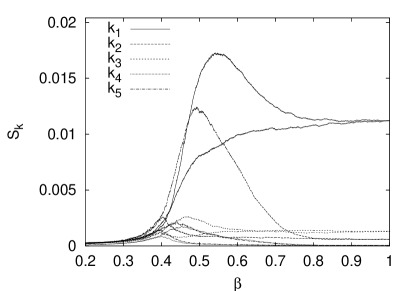
Figure 15: Hysteresis of the $S_{k}(t)$ structure functions for the 2-state Potts model on an $80\times 80$ lattice ($n_{\beta}=1$).

Figure 16: Time evolution of the $S_{k}(t)$ structure functions for the 10-state Potts model on an $80\times 80$ lattice after quenching from $\beta_{\min}=0.4$ to $\beta_{\max}=0.8$.

Figure 17: Time evolution of the $S_{k}(t)$ structure functions for the 2-state Potts model on an $80\times 80$ lattice after quenching from $\beta_{\min}=0.2$ to $\beta_{\max}=0.6$.

Figure 18: Time evolution of the $S_{k}(t)$ structure functions for the 2-state Potts model on an $80\times 80$ lattice after quenching from $\beta_{\min}=0.2$ to $\beta_{\max}=0.6$ at a magnetic field $h=0.01$.

Miller and Ogilvie MiOg02 investigated the dynamics of SU(2) gauge theory after quenching from a low to a high physical temperature (corresponding to the $\beta_{\min}\to\beta_{\max}$ half-cycle of the spin system). They report a critical value $k_{c}$, so that modes grow (do not grow) exponentially for $k<k_{c}$ ($k>k_{c}$).

In figures 14 and 15 we show for our $n_{\beta}=1$ dynamics all structure functions, which we have measured. It is notable that we observe a large gap between the peaks for $S_{k_{i}}(\beta)$, $i=1,2$ and for $S_{k_{j}}(\beta)$, $j\geq 3$. We also performed quenching runs. In figure 16 we show the time evolution on an $80\times 80$ lattice after quenching the 10-state Potts model from $\beta=0.4$ to $\beta=0.8$ and in figure 17 we show the time evolution after quenching the 2-state Potts model from $\beta=0.2$ to $\beta=0.6$. As in our hysteresis investigations averages of 640 independent repetitions are taken. Again, we find a large gap between the peaks for $S_{k_{i}}(\beta)$, $i=1,2$ and for $S_{k_{j}}(\beta)$, $j\geq 3$. Further it is remarkable that the height of the peaks in the hysteresis cooling half-cycles and under quenching are almost identical, while the time scale is according to equation (7) extended to 3200 sweeps for the hysteresis curve.

For figure 18 we have changed the second order phase transition of the 2-state Potts model to a crossover by adding the term $h\sum_{\vec{r}}\delta_{\sigma(\vec{r},t),\,q_{0}}$ with a small magnetic field $h$, $h=0.01$, with respect to the spin $q_{0}$ in the Hamiltonian (1). In essence the time evolution after quenching is similar as without the magnetic field, only that the magnitude of the $S_{k_{1}}$ and $S_{k_{2}}$ peaks decreases, maintaining still a clearly visible gap to the peaks of the $S_{k_{j}}$, $j\geq 3$ structure functions. Increasing the magnetic field further, to $h=0.1$, the large peaks disappear altogether by merging into the small peaks. The signal of a transition is possibly lost for such high values of the magnetic field.

The observed peaks suggest a critical $k_{i}$ value between $i=2$ and $i=3$ for the Potts models. However, the issue is more subtle. Cahn-Hilliard theory CaHi58 ; Ca68 (model B for reviews see ChLu97 ; La92 ; Gu83 ) predicts an exponential growth of the low momentum structure function in the initial part of the time evolution after quenching (also applies to model A). Whether such an exponential growth is found or not was used by Miller and Ogilvie MiOg02 to determine the critical $k_{c}$ between the low and the high momentum mode. However, none of our structure functions in figures 16 to 18 shows initial exponential growth. This is already kind of obvious by looking at the figures, where the shape of the increasing parts of the curves is always concave and is quantitatively determined by performing fits. A likely explanation is that the Cahn-Hilliard theory relies on approximations which are not justified in our $2d$ models. In $3d$ we find exponential growth in the very early stage of the time evolution after quenching (incrementing then $\beta$ after every update and fitting the time evolution within the first sweep BV ). Interestingly, our hysteresis curves of figures 14 and 15, which rely on the smoother dynamics of temperature changes in small steps, show an initial exponential growth.

We find no peaks in the structur factors when we quench from an ordered initial state into the disordered phase. The reason may be that the structure factor is defined with respect to the order parameter. Under a quench into the ordered phase $q$-ality order-order domain may emerge, whereas there is only one disordered phase.

IV Summary and Conclusions

Our energy hysteresis method allows for dynamical estimates of the equilibrium transition temperatures for first as well as for second order phase transitions. While the precision of these estimates is not competitive with those of equilibrium investigations, the hysteresis method provides information about dynamically rooted deviations of accompanying physical observables from their equilibrium values. For second order transitions we find that the dynamics generates a latent heat and for a weak first order transition we find a ‘dynamical’ latent heat much larger than its equilibrium value, whereas for a strong first order transition the dynamical latent heat agrees with the equilibrium value (the magnetization allows for a similar analysis, which is not reported here).

In our analysis of $2d$ Potts models, we find spinodal decomposition to be the dominant feature as soon as we turn on the dynamics. For instance, the equilibrium (quasi static) phase conversion of first order phase transitions is due to nucleation. Even our slowest dynamics ($n_{\beta}=16$) changes the phase conversion of the investigated weak ($q=5$) and strong ($q=10$) first order transitions from nucleation to spinodal. For the $q=2$ (weak) second order transition the $n_{\beta}=16$ dynamics appears to be already rather close to equilibrium, which is formally reached for $n_{\beta}\to\infty$. These results are mainly based on analyzing the dynamical time evolution of Fortuin-Kasteleyn (FK) clusters and structure functions.

• For FK clusters we find that the largest cluster surface area is quite sensitive to dynamical effects and yields for all considered $q$-values signals in favor of a spinodal decomposition on the cooling ($\beta\to\beta_{\max}$) and heating ($\beta\to\beta_{\min}$) half-cycles of our hysteresis loops. This may be illustrated by comparing the results of our fast ($n_{\beta}=1$) dynamics of figure 8 with the equilibrium results of figure 6. For the first order transitions the dynamics enhances the peak values to take on similar values as one finds for the $q=2$ and $q=4$ second order configurations near the critical point.

• For the structure factor our $n_{\beta}=1$ dynamics leads on the $\beta_{\min}\to\beta_{\max}$ half-cycle to amplitude maxima, which are considerably larger than those from the second order equilibrium configurations, see figure 11. The dynamical peaks on the $\beta_{\max}\to\beta_{\min}$ half-cycle are comparable to those of from the equilibrium configurations, which has for figure 11 the consequence that they are not visible at all, because the systems are still out of equilibrium at $\beta_{\max}$ and on their return path. That is of potential interest for heavy ion collision, where our $\beta_{\min}\to\beta_{\max}$ half cycle corresponds to heating for which the dynamics of the experiment is definitely fast. We have no entirely satisfactory theoretical explanation for the observed asymmetry, but think that is is related to the fact that $q$-ality order-order domain may emerge in the ordered (deconfined) phase.

Using quenching, we find dynamical signals surviving even after the proper (second order) phase transition is converted into a crossover. Moving then far away from the transition, the dynamical signals fade away too and the issue of crossovers requires further investigations.

Our computer programs allow to extend the present study to the 3-state Potts model in three dimensions with an external magnetic field representing quark effects. In a more remote future, one could carry out similar studies for quenched and even full QCD. But none of these studies could resolve the problem of a quantitative relationship between the Glauber time scale of our Euclidean dynamics and the time scale of the Minkowskian dynamics in the real world. In this context it is of interest that Pisarski and Dumitru developed recently a Polyakov loop model DuPi01 which allows for simulations in the Minkowskian formulation Sc01 . It may be possible to address questions similar to those raised in our paper within the hyperbolic dynamics of their model.

Most likely the aim of such studies cannot be to make precise quantitative predictions. Instead, one may have to be content with illustrating the effect of different speeds of the phase conversion on the observable signals qualitatively. If spinodal decomposition of Polyakov loops is indeed realized in heavy ion collisions, one may observe an enhancement in the production of low-energy gluons.

- (1) S. Ejiri, Nucl. Phys. Proc. Suppl. 94 (2001) 19; F. Karsch, Lect. Notes Phys. 583 (2002) 209; H. Meyer-Ortmanns, Rev. Mod. Phys. 68 (1996) 473.
- (2) Ch. Schmidt, C.R. Allton, S. Ejiri, S.J. Hands, O. Kaczmarek, F. Karsch and E. Laermann, Nucl. Phys. B. (Proc. Suppl.) 119 (2003) 517; F. Karsch, AIP Conf. Proc. 602 (2001) 323 (hep-lat/0109017); F. Karsch, E. Laermann, and Ch. Schmidt, Phys. Lett. B 520 (2001) 41. F.R. Brown, F.P. Butler, H. Chen, N.H. Christ, Z. Dong, W. Schaffer, L.I. Unger, and A. Vaccino, Phys. Lett. B 251 (1990) 181;
- (3) H. Meyer-Ortmanns and B.-J. Schaefer, Phys. Rev. D 53 (1996) 6586-6601.
- (4) T.R. Miller and M.C. Ogilvie, Nucl. Phys. B (Proc. Suppl.) 106 (2002) 357; Phys. Lett. B 488 (2000) 313.
- (5) R. Anishetty, P. Koehler, and L. McLerran, Phys. Rev. D 22 (1980) 2793.
- (6) J.D. Bjorken, Phys. Rev. D 27 (1983) 140 and references given therein.
- (7) J.D. Bjorken, Int. J. Mod. Phys. A 7 (1992) 4189; J.D. Bjorken, K.L. Kowalski and C.C. Taylor, hep-ph/9309235.
- (8) K. Rajagopal and F. Wilczek, Nucl. Phys. B 399 (1993) 395; 404 (1993) 577; F. Wilczek, Nucl. Phys. A 566 (1994) 123.
- (9) B.A. Berg, U.M. Heller, H. Meyer-Ortmanns, and A. Velytsky, hep-lat/0308032, to appear in the Proceedings of the Tsukuba Lattice 2003 Conference, Nucl. Phys. B (Proc. Suppl).
- (10) A.M. Polyakov, Phys. Lett. B72 (1978) 477.
- (11) B. Svetitsky and L.G. Yaffe, Nucl. Phys. B 210 (1982) 423.
- (12) M. Gross, J. Bartholomew, and D. Hochberg, Phys. Lett. B 113 (1983) 218.
- (13) M. Ogilvie, Phys. Rev. Lett. 52 (1984) 1369.
- (14) A. Gocksch and M. Ogilvie, Phys. Rev. D 31 (1985) 877.
- (15) T. Banks and A. Ukawa, Nucl. Phys. B 225 [FS9] (1983) 145.
- (16) R.J. Baxter, J. Phys. C6 (1973) L445.
- (17) C. Borgs and W. Janke, J. Phys. I France 2 (1992) 2011, and references given therein.
- (18) F.Y. Wu, Rev. Mod. Phys. 54 (1982) 235.
- (19) R.J. Glauber, J. Math. Phys. 4 (1963) 294; K. Kawasaki, in Phase Transitions and Critical Phenomena, C. Domb and M.S. Green (editors), Vol. 2 (1972) 443.
- (20) P.M. Chaikin and T.C. Lubensky, Principles of condensed matter physics, Cambridge University Press, Cambridge, 1997.
- (21) H.J. Rothe, Lattice Gauge Theories – An Introduction, World Scientific Lecture Notes in Physics Vol.43 (Chapter 17), Singapore, 1992, and references given therein.
- (22) C.M. Fortuin and P.W. Kasteleyn, Physica 57 (1972) 536; A. Coniglia and W. Klein, J. Phys. A13 (1980) 2775.
- (23) B.A. Berg, H. Meyer-Ortmanns, and A. Velytsky, in preparation.
- (24) M. Creutz, L. Jacobs and C. Rebbi, Phys. Rev. Lett. 42 (1979) 1390.
- (25) R.H. Swendsen and J. Wang, Phys. Rev. Lett. 58 (1987) 86.
- (26) J.W. Cahn, Trans. Metall. Soc. AIME 242 (1968) 166.
- (27) M. Hillert, Acta Met. 9 (1961) 525.
- (28) J.S. Langer in ”Solids far from Equilibrium”, C. Godreche (editor), Cambridge University Press, Cambridge, 1992.
- (29) J.D.Gunton, M. San Miguel and P.S. Sahni, in ”Phase Transitions and Critical Phenomena”, Vol.8, C. Domb and J.L. Lebowitz (editors), Academic Press, London, 1983.
- (30) A. Velytsky, Ph.D. thesis, in preparation.
- (31) J. Kertész, Physica A161 (1989) 58.
- (32) D. Stauffer and A. Aharony, Introduction to Percolation Theory, Taylor & Francis, London 1994.
- (33) H. Satz, Comp. Phys. Commun. 147 (2002) 40, and references given therein.
- (34) H.E. Stanley, Introduction to Phase Transitions and Critical Phenomena, Clarendon Press, Oxford, 1972, p.98–p.100 and p.204–p.210.
- (35) A. Velytsky, B.A. Berg and U. Heller, Nucl. Phys. B (Proc. Suppl.) 119 (2003) 861.
- (36) M.E. Fisher, in Nobel Symposium 24, edited by B. Lundquist and S. Lundquist (Academic Press, New York, 1974).
- (37) B.A. Berg and T. Neuhaus, Phys. Rev. Lett. 68 (1992) 9.
- (38) A. Billoire, T. Neuhaus and B.A. Berg, Nucl. Phys. B 396 (1993) 779; B 413 (1994) 795; T. Neuhaus and J.S. Hager, J. Stat. Phys. 113 (2003) 47.
- (39) H.W.J. Blöte and M.P. Nightingale, Phys. Rev. B 62 (2000) 1089.
- (40) J.W. Cahn and J.E. Hilliard, J. Chem. Phys. 28 (1958) 258.
- (41) R.D. Pisarski, Phys. Rev. D 62 (2000) 111501(R); A. Dumitru and R. Pisarski, Phys. Lett. B 504 (2001) 282.
- (42) O. Scavenius, A. Dumitru and A.D. Jackson, Phys. Rev. Lett. 87 (2001) 182302