Matrix elements of decays††thanks: Presented by Mauro Papinutto at Lattice 2003
Abstract
We present a numerical computation of matrix elements of decays by using Wilson fermions. In order to extrapolate to the physical point we work at unphysical kinematics and we resort to Chiral Perturbation Theory at the next-to-leading order. In particular we explain the case of the electroweak penguins which can contribute significantly in the theoretical prediction of . The study is done at on a lattice.
1 INTRODUCTION
The study of non-leptonic kaon decays is a challenging but important task, which is underlined by the recent accurate measurement of a non-zero parameter [1] (the first confirmed observation of direct CP violation) and the long-standing puzzle of the rule.
For example, the electroweak penguins (EWPs)
although suppressed by the factor when compared to the QCD penguins, are enhanced by the rule and tends to cancel significantly the contribution of the QCD penguins in the theoretical prediction of .
Here we present the first lattice determination of the matrix elements (MEs) of the EWPs obtained directly with a two-pion final state. The strategy, explained in [2, 3], consists in computing at some unphysical kinematics on the lattice (called SPQR kinematics) and then using next-to-leading order (NLO) Chiral Perturbation Theory (PT) to obtain the MEs at the physical point.
2 OPERATOR MATCHING
We now discuss the problem of the matching of lattice-regularised operators to the continuum renormalization scheme in which the Wilson coefficients are calculated. Even if chirality is preserved by the regularization, and (the parts of ) mix between themselves. In a Wilson-like regularization there is in general also mixing with operators of different naive chiralities. In the case, isospin symmetry forbids mixing with lower dimensional operators while symmetry implies that mixing with other dimension six operators with different chiral properties occurs only in the parity conserving sector [5]. The mixing is thus:
| (5) |
where is the renormalization scale. With an obvious notation we define , , , to be the MEs of .

To compute we use the (mass independent) RI-MOM renormalization scheme which can be easily implemented in a non-perturbative way, also in the case of four fermion operators [5]. Spurious effects due to the Goldstone boson contamination have been removed by using the method explained in [6, 2].
Once computed non-perturbatively, we have to check to what extent it follows the renormalization group behaviour predicted by perturbation theory at the NLO. We thus compute
| (6) |
The observation that no clear lattice artifacts are visible in , together with the very large anomalous dimension of , (6 and 16 at LO) suggest that higher orders in PT could contribute significantly in particular to the RG evolution of .
The central value for the renormalization constants at a given scale is extracted in the following way: we compute by fitting the plateaux to a constant in the interval . We then run down to the desired scale . The systematic error is estimated by computing the variation of the value obtained at this scale from the evolution of the original values (those used to build the combination of Eq. 2 and Fig. 1) at the different scales .
3 USE OF THE CHIRAL EXPANSION
| fit | |||||
|---|---|---|---|---|---|
| poly. | 0.120(11) | 0.023 | 0.714(62) | 0.031 | |
| poly. | 0.125(13) | 0.012 | 0.715(75) | 0.037 | |
| PT | 0.143(13) | 0.817 | 0.836(73) | 0.815 | |
| PT | 0.123(13) | 0.482 | 0.700(72) | 0.626 | |
| qPT | 0.254(25) | 13.2 | 1.49(16) | 10.8 | |
| qPT | 0.212(24) | 5.95 | 1.19(14) | 4.91 |
The NLO contribution in PT, both in the quenched approximation and in the full-QCD case, has been computed for the SPQR kinematics in [4]. One can thus think of extracting the low energy constants (LECs) of the LO and NLO (in the case of the EWPs and respectively) from lattice data and to use them in the NLO formula for the physical kinematics. Both forms can be derived from the formula in the most general kinematics (energy momentum injection via the weak operator allowed but with all the particles on-shell) which reads
| (7) |
where we have symmetrized over , since the two pion state is a pure state.
The SPQR kinematics corresponds to put the and one at rest while the other is either at rest or has the minimum momentum allowed on the lattice. The previous formula can thus be re-expressed in terms of , and , where is the energy of the (possibly) moving pion.
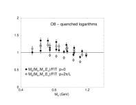
Besides the fit with the complete form predicted by PT (Eq. 7), we also try a fit with the polynomial part only (the coefficients of which are now “effective” LECs) which we call . Tab. 1 reports the results of the fits. It is clear by looking at the that our data are not in the kinematical range where the chiral logarithms are visible. This is visualized in Fig. 2.a-b. A possible explanation for this behaviour is that, since logarithms come from loops of Goldstone bosons (GBs), they become relevant at a scale of the order of the mass of the GBs. Since the contribution of the counterterms is instead controlled by the physics at the scale of the cut-off (i.e. ), it is dominant in the kinematical region accessible on the lattice (in our simulation ).
| poly. | ||||
|---|---|---|---|---|
| match. | PT | qPT | PT | qPT |
| 0.3,0.5 | ||||
| 0.4,0.5 | ||||
| 0.3,0.31 | ||||
| 0.5,0.51 | ||||
On the other hand, one expects that predictions of PT (including the logs.) are valid when all the energy scales are sufficiently small (let’s say below the mass of the Kaon). If we assume that there exists a region in which the two descriptions of the form factors are reasonably close to each other, we can perform the matching between these two forms [8]. This amounts to fit the data with and then to impose the equality of with and of their first derivatives with respect to the kinematical variables , , , at a matching point (chosen in the SPQR kinematics).
Results for different matching points are shown in Tab. 2. Lattice data have not yet been corrected for all of the finite volume corrections explained in [2] and so our results are still preliminary. Nevertheless it’s interesting to study the systematics of the PT-polynomial matching and the contribution of the NLO at the physical point. Since quenched logarithms are very different from the full QCD ones (and assuming that quenching does not change drastically the kinematical behaviour of the form factors in the range accessible to the lattice) we think that the most sensible way of extrapolating to the physical point is to perform the matching with full PT. If we choose the matching point ()=(0.4,0.5) GeV we get:
where the first error is statistical, the second is the systematics of non-perturbative renormalization and the third is the systematics due to the variation of the matching point. At the physical point, the NLO gives a negative contribution of order with respects to the LO.
References
- [1] J. R. Batley et al. [NA48 Coll.], Phys. Lett. B544 (2002) 97, A. Alavi-Harati et al. [KTeV Coll.], Phys. Rev. D67 (2003) 012005.
- [2] P. Boucaud et al. [SPQR Coll.], Nucl. Phys. Proc. Suppl. 106 (2002) 323-325 and 329-331.
- [3] D. Becirevic et al. [SPQR Coll.], Nucl. Phys. Proc. Suppl. 119 (2003) 359-361.
- [4] C.-J. D. Lin et al., Nucl. Phys. B650 (2003) 301.
- [5] A. Donini et al., Eur. Phys. J. C10 (1999) 121.
- [6] D. Becirevic et al., JHEP 0204 (2002) 025.
- [7] M. Ciuchini et al., Nucl. Phys. B523 (1998) 501.
- [8] A. S. Kronfeld and S. M. Ryan, Phys. Lett. B543 (2002) 59, D. Becirevic, S. Prelovsek and J. Zupan, Phys. Rev. D67 (2003) 054010.