DESY 03-149
SFB/CPP-03-39
September 2003

Pion parton distribution functions from lattice QCD

Abstract

We report on recent results for the pion matrix element of the twist-2 operator corresponding to the average momentum of non-singlet quark densities. For the first time finite volume effects of this matrix element are investigated and come out to be surprisingly large. We use standard Wilson and non-perturbatively improved clover actions in order to control better the extrapolation to the continuum limit. Moreover, we compute, fully non-perturbatively, the renormalization group invariant matrix element, which allows a comparison with experimental results in a broad range of energy scales. Finally, we discuss the remaining uncertainties, the extrapolation to the chiral limit and the quenched approximation.

1 INTRODUCTION

Parton distribution functions of hadrons are in the focus of several theoretical and experimental investigations. In recent years lattice QCD calculations have provided estimates for the lowest moments of parton distribution functions, but so far most of the results have been obtained at one fixed lattice spacing only and using perturbative renormalization factors for the bare operators.

The scope of our current investigation is the pion matrix element of the twist-2 operator corresponding to the average momentum of non-singlet quark densities. This operator belongs to two irreducible representations of the lattice $H(4)$ group. We will concentrate solely on the matrix element of the operator

$${\cal O}_{44}(x) = \bar{\psi}(x)\Big{[}\gamma_{4}\stackrel{{\scriptstyle\leftrightarrow}}{{D}}_{4}-\frac{1}{3}\sum_{k=1}^{3}\gamma_{k}\stackrel{{\scriptstyle\leftrightarrow}}{{D}}_{k}\Big{]}\frac{\tau^{3}}{2}\psi(x)\;,$$

since it can be computed at zero external pion momentum and thus provides a reliable signal. In particular we use Schrödinger functional (SF) boundary conditions [1] for our computation, which allows the extraction of the matrix element from one large plateau around the middle of the time extent $T$ of the lattice. The correlation function of the matrix element $f_{M}$ is obtained by inserting the ${\cal O}_{44}$ operator between two SF pion states ${\cal O}_{0}$ and ${\cal O}_{T}$ at the time boundaries $t=0$ and $T$ and suitable normalization with the boundary-to-boundary correlator $f_{1}$ [2, 3]

$$f_{M}(t) = a^{3}\sum_{\rm x,y,z}\langle{\cal O}_{0}\;{\cal O}_{44}(x)\;{\cal O}_{T}\rangle$$

$$\sim e^{-m_{\pi}T}\;\langle\pi|{\cal O}_{44}|\pi\rangle\;\{1+\dots\}$$

$$f_{1} = -\langle{\cal O}_{0}{\cal O}_{T}\rangle\;\sim\;e^{-m_{\pi}T}\;.$$

The bare pion matrix element is then defined by

$$\langle x\rangle^{bare}\equiv\frac{2\kappa}{m_{\pi}}\langle\pi|{\cal O}_{44}|\pi\rangle=\frac{2\kappa}{m_{\pi}}f_{M}(t)/f_{1}\;,$$

considering a plateau region around $T/2$ where the relative excited state contribution $\epsilon$ is below 0.4%. The pion mass is obtained from the time dependence of the improved axial-vector correlator $f^{I}_{A}$ following [2] and requiring $\epsilon$ smaller than 0.1%.

2 FINITE VOLUME EFFECTS

Finite volume effects for pion and nucleon matrix elements have not been studied before, but might influence the precise determination of moments of parton distribution functions from lattice QCD. We have investigated the effects of limited lattice extent in detail at $\beta$=6.1 ($a$=0.079 fm) with the non-perturbatively improved clover fermion action and lattice sizes ranging from $12^{3}\times 36$ to $32^{3}\times 56$.

While the pion mass reaches a constant value already for $L\simeq 1.2$ fm and $T\simeq 2.8$ fm (see figure 1), the bare pion matrix element in figure 2 shows very strong finite volume effects. For the largest quark mass $L\simeq 1.6$ fm and $T\simeq 3.2$ fm seems to be sufficient, whereas an even larger spatial extent of 1.9 fm is needed for the smallest quark mass. The lines in both figures represent exponential fits with the purely phenomenological ansatz $X(L)\!=\!c_{0}+c_{1}/L^{3/2}\exp(-c_{2}L)$, where $X\!\!=\!\!m_{\pi}a$ or $\langle x\rangle$. Please note that a power-law fit ansatz would describe the data almost equally well.

These observations lead to the expectation that the finite volume effects for nucleon matrix elements could be even larger, since the influcence of the limited lattice size on the nucleon mass has already been observed to be much stronger than for the pion mass [4]. This might be one ingredient for the deviation of current lattice QCD estimates of $\langle x\rangle$ for the nucleon in comparison with experimental data.

Figure 1: Finite volume effects for $m_{\pi}a$

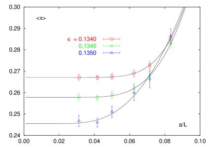
Figure 2: Finite volume effects for $\langle x\rangle$

3 CONTINUUM EXTRAPOLATION

In order to improve the continuum extrapolation we use both the unimproved Wilson and non-perturbatively improved clover fermion action, which can have different ${\cal O}(a)$ effects due to the usage of the unimproved ${\cal O}_{44}$ operator, but should agree in the continuum limit. We have complemented a previous data set [3] with simulations at $\beta$=6.1 $(24^{3}\times 42)$ and $\beta$=6.45 $(32^{3}\times 72)$. The bare matrix elements were renormalized with the appropriate Z factors computed non-perturbatively at the same low energy scale $\mu_{0}$ in the SF scheme [5]. In figure 3 we show the combined continuum extrapolation (4 smaller lattice spacings) of the renormalized matrix element

$$\langle x\rangle^{ren}_{SF}(\mu_{0})=\lim_{a\to 0}\lim_{m\to 0}\frac{\langle\pi|{\cal O}_{44}|\pi\rangle(a)}{Z_{SF}(1/\mu_{0},a)}\;,$$

where the chiral extrapolation had been performed linearly in the quark mass. This yields a value of $\langle x\rangle^{ren}_{SF}(\mu_{0})=0.870(33)$ for the renormalized pion matrix element in the SF scheme.

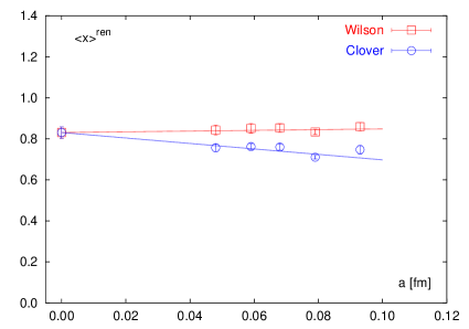
Figure 3: Combined continuum extrapolation for different discretizations of the fermion action

4 RGI MATRIX ELEMENT

The phenomenological analysis of the experimental data is usually done in the $\overline{MS}$ scheme. In order to translate our fully non-perturbatively computed matrix element $\langle x\rangle^{ren}_{SF}(\mu_{0})$ renormalized in the SF scheme to the $\overline{MS}$ scheme, we need first to calculate the universal renormalization group invariant (RGI) matrix element. This is done following the complete non-perturbative evolution [5] in the SF scheme until it is possible to make (at small volumes) a matching with perturbation theory. Using the so-called UV-invariant step scaling function it is then possible to eliminate any reference to the scale $\mu_{0}$ and obtain finally the RGI matrix element

$${\langle x\rangle}^{RGI}={\langle x\rangle}^{ren}_{SF}(\mu_{0})\;\sigma^{UV}_{INV}(\mu_{0})=0.192(11)\;.$$

The RGI matrix element allows a simple conversion to any desired scheme (e.g.$\;\overline{MS}$ at 2GeV) requiring only the knowledge of the $\beta$- and $\gamma$-function up to a certain order in perturbation theory in this scheme [5]. The resulting number $\langle x\rangle_{\overline{MS}}(\mu$=2GeV)=0.265(15) has decreased slightly compared to the previous lattice computation [6] $\langle x\rangle_{\overline{MS}}(\mu$=2.4GeV)=0.273(12), which has been performed only at one lattice spacing and with perturbative renormalization factors.

5 LIMITATIONS

Our new result is still higher, but already more precise than the latest NLO analyses of Drell-Yan and prompt photon $\pi N$ data [8, 9], which yield a combined experimental value of $\langle x\rangle_{\overline{MS}}(\mu$=2GeV) = 0.21(2). The quenched approximation is certainly one limitation that has to be explored in the future.

Another aspect that has been investigated recently is the chiral extrapolation. It has been shown [7] that a non-linear fit of the previous data [6] leads to $\langle x\rangle_{\overline{MS}}=0.24(1)(2)$, which is much more compatible with the experimental number. The first error is the statistical and the second describes the variation with the fit parameters.

In figure 4 we show our results performing first the combined continuum extrapolation of Wilson and clover data at fixed $m_{\pi}^{2}$. A linear chiral fit yields a consistent result $\langle x\rangle_{\overline{MS}}=0.263(14)$ with interchanged limits, while a non-linear fit similar to [7] yields $\langle x\rangle_{\overline{MS}}=0.22(1)(2)$ and is thus compatible within error with the experimental number. Despite these results the correct chiral extrapolation needs further investigations, especially in the region of smaller and realistic quark masses.

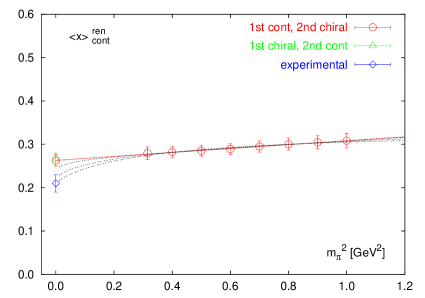
Figure 4: Comparison of chiral expolations: linear (solid line) and non-linear [7] with $\Lambda$=0.4, 0.7, 1.0 GeV (dotted lines)

References

-
[1]
M. Lüscher et al., NPB 384 (1992) 168;
S. Sint, NPB 421 (1994) 135 - [2] M. Guagnelli et al. (ALPHA Collaboration), NPB 560 (1999) 465
- [3] M. Guagnelli, K. Jansen, R. Petronzio, PLB 493 (2000) 77
- [4] S. Aoki et al., PRD 50 (1994) 486
- [5] M. Guagnelli et al. (ZeRo Collaboration), NPB 664 (2003) 276; A. Shindler et al. (ZeRo Collaboration), these proceedings
- [6] C. Best et al., PRD 56 (1997) 2743
- [7] W. Detmold, W. Melnitchouk, A.W. Thomas, hep-lat/0303015
- [8] P.J. Sutton, A.D. Martin, R.G. Roberts, W.J. Stirling, PRD 45 (1992) 2349
- [9] M. Glück, E. Reya, I. Schienbein, Eur.Phys.J. C10 (1999) 313