Baryons and Confining Strings

Abstract

The subleading term of the heavy quark potential (the analogue of the Lüscher term) is computed in a string model for the case of three quarks. It turns out to be positive in 2+1 dimensions, making the potential non-concave as a function of the scale for fixed geometry. The results are compared to numerical simulations of the lattice gauge theory.

1 Motivation

The potential of three heavy quarks has recently been the object of detailed numerical studies [1, 2], which lend support to the so-called Y law, inspired by a string picture of heavy baryons. Here, we study the leading effect of string fluctuations on the potential, the analogue of the Lüscher term [3, 4, 5] in the quark-antiquark potential. Understanding such corrections to the Y law is particularly important since the transition from $\Delta$ to Y law occurs at large quark separations [1].

2 Setup

We study three static quarks in a $D$-dimensional Euclidean space with periodic Euclidean time extent $T$. The potential is obtained from the $T\to\infty$ limit,

$$V_{{\textrm{q}}{\textrm{q}}{\textrm{q}}}=-\lim_{T\to\infty}\frac{1}{T}\ln Z_{{\textrm{q}}{\textrm{q}}{\textrm{q}}}\;.$$ (1)

In the string picture, the classical ground state of the three-quark system is given by three strings meeting at a junction, whose position is determined by the requirement of minimal total length of the strings. The balance of tensions implies angles of $\frac{2\pi}{3}$ between the strings. The classical potential is proportional to the total length of the strings in this configuration,

$$V_{\text{cl}}=\sigma(L_{1}+L_{2}+L_{3})+m=\sigma L_{\textrm{Y}}+m\;,$$ (2)

where $\sigma$ is the same string tension that appears in the mesonic potential. $m$ represents the self-energy of the junction.

Following the mesonic case [4], we shall expand the action to second order in the transverse fluctuations $\vec{\xi}_{a}(t,s)$ of the string world sheets $a=1,2,3$ around the classical configuration. Transversality means $\xi_{a}^{D}=0$ and $\vec{e}_{a}\cdot\vec{\xi}_{a}=0$, where $\vec{e}_{a}$ is a spatial unit vector in the direction of string $a$. With $\vec{\phi}(t)$ denoting the position of the fluctuating junction, the boundary conditions are

$$\vec{\xi}_{a}(t,0)=\vec{x}_{a}\;,\quad\vec{\xi}_{a}\bigl{(}t,L_{a}+\vec{e}_{a}{\cdot}\vec{\phi}(t)\bigr{)}=\vec{\phi}_{\perp a}(t)\;,$$ (3)

where $\vec{\phi}_{\perp a}\equiv\vec{\phi}-\vec{e}_{a}(\vec{e}_{a}\cdot\vec{\phi})$, and periodic in $t$.

Invariance under Euclidean transformations inside the plane of the sheet and perpendicular to it fixes the leading term in a derivative expansion of the bulk string action to

$$S_{\textrm{fluct}}^{\text{bulk}}=\frac{\gamma}{2}\sum_{a=1}^{3}\int_{\Gamma_{a}}\!\partial\vec{\xi}_{a}\cdot\partial\vec{\xi}_{a}\;,$$

where $\Gamma_{a}$ is the domain of $\xi_{a}$ implied by the boundary conditions (3). We also include a boundary term,

$$S_{\textrm{fluct}}^{\text{bound}}=\frac{\mu}{2}\int\!{\mathrm{d}}t\,|\dot{\vec{\phi}}|^{2}\;.$$

The change of area caused by fluctuations of the junction in the plane of a given sheet cancels in the sum over sheets. The three-quark potential including leading fluctuation effects can thus be extracted from the partition function

$$Z_{{\textrm{q}}{\textrm{q}}{\textrm{q}}}=\int\!{\mathrm{D}}\vec{\phi}\int\prod_{a=1}^{3}{\mathrm{D}}\vec{\xi}_{a}\,{\mathrm{e}}^{-TV_{\text{cl}}-S_{\textrm{fluct}}^{\text{bulk}}-S_{\textrm{fluct}}^{\text{bound}}}.$$ (4)

3 Calculation

We shall compute $Z_{{\textrm{q}}{\textrm{q}}{\textrm{q}}}$ in two steps. For fixed $\vec{\phi}$, each of the string partition functions,

$$Z_{a}(\vec{\phi})=\int\!{\mathrm{D}}\xi_{a}\,\exp\left\{\textstyle-\frac{\gamma}{2}\int|\partial\vec{\xi}_{a}|^{2}\right\}\;,$$

splits into a minimal-area and a fluctuation part,

$$Z_{a}(\vec{\phi})={\mathrm{e}}^{-\frac{\gamma}{2}\int|\partial{\vec{\xi}_{a,{\textrm{min}}}}|^{2}}\;\left|\det\nolimits_{\Gamma_{a}}\bigl{(}{-\Delta}\bigr{)}\right|^{-\frac{D-2}{2}}\;,$$

where $\vec{\xi}_{a,{\textrm{min}}}$ is harmonic and satisfies (3) and the determinant is computed with Dirichlet boundary conditions on the domain $\Gamma_{a}=\{(t,s)\mid 0\leq s\leq L_{a}+\vec{e}_{a}\cdot\vec{\phi}(t)\}$.

To leading order in $\vec{\phi}$,

$$\vec{\xi}_{a,{\textrm{min}}}=\frac{1}{\sqrt{T}}\sum_{\omega}\vec{\phi}_{\omega}^{\perp}\,\frac{\sinh(\omega s)}{\sinh(\omega L_{a})}\,{\mathrm{e}}^{{\mathrm{i}}\omega t}+{\mathcal{O}}(\phi^{2})\;,$$

where $\vec{\phi}_{\omega}$ are the Fourier components of $\vec{\phi}(t)$. This implies

$$\int|\partial\vec{\xi}_{a,{\textrm{min}}}|^{2}=\sum_{\omega}\omega\coth(\omega L_{a})\,|\vec{\phi}_{\omega}^{\perp}|^{2}+{\mathcal{O}}(\phi^{3})\;,$$

which is the change in minimal area due to $\vec{\phi}_{\perp a}$.

The determinant induces a renormalisation of both $\sigma$ and $m$. After applying a Pauli–Villars regularisation, the determinant, which can be expressed in terms of the heat kernel of $\Delta$, can be computed by mapping the domain $\Gamma_{a}$ conformally to a rectangle $L_{a}^{\prime}\times T$. Since the conformal map cannot change the ratio $L_{a}^{\prime}/T$ (the modular parameter of the cylinder), one has to choose $L_{a}^{\prime}=L_{a}+\frac{1}{T}\int\vec{e}_{a}\cdot\vec{\phi}\,{\mathrm{d}}t$. To leading order in $\vec{\phi}$, the conformal map is

$$f(z)=z+\frac{1}{\sqrt{T}}\sum_{\omega\neq 0}\frac{\vec{e}_{a}\cdot\vec{\phi}_{\omega}}{\sinh(\omega L_{a})}\,{\mathrm{e}}^{\omega z}+{\mathcal{O}}(\phi^{2})\;.$$

Following Ref. [3], the determinant on $\Gamma_{a}$ can be related to that on the rectangle, and one finds

$$\ln\det\nolimits_{\Gamma_{a}}(-\Delta)=2\ln\eta\!\left(\frac{{\mathrm{i}}\,T}{2L_{a}^{\prime}}\right)\\ -\frac{1}{12\pi}\sum_{\omega}\omega^{3}\coth(\omega L_{a})\,|\vec{e}_{a}{\cdot}\vec{\phi}_{\omega}|^{2}\;+\;{\mathcal{O}}(\phi^{3})\;,$$

where $\eta$ is Dedekind’s function.

The Gaussian integral over $\vec{\phi}$ in (4) can now be performed and $V_{{\textrm{q}}{\textrm{q}}{\textrm{q}}}$ be extracted from the limit $T\to\infty$, cf. (1). One obtains:

$$\mskip-36.0muV_{{\textrm{q}}{\textrm{q}}{\textrm{q}}} =V_{\text{cl}}^{\text{ren}}+V_{1/L}^{\parallel}+(D{-}3)V_{1/L}^{\perp}\;+{\mathcal{O}}(L^{-2})\;,$$

$$\mskip-36.0muV_{1/L}^{\parallel} ={-\frac{\pi}{24}\sum_{a}\frac{1}{L_{a}}}$$

$$\mskip 12.0mu+\int\limits_{0}^{\infty}\!\frac{{\mathrm{d}}\omega}{2\pi}\ln\biggl{[}\tfrac{1}{3}\sum_{a<b}{\coth(\omega L_{a})\coth(\omega L_{b})}\biggr{]}\;,$$

$$\mskip-36.0muV_{1/L}^{\perp} ={-\frac{\pi}{24}\sum_{a}\frac{1}{L_{a}}}$$

$$\mskip 12.0mu+\int\limits_{0}^{\infty}\!\frac{{\mathrm{d}}\omega}{2\pi}\ln\biggl{[}\tfrac{1}{3}\sum_{a}{\coth(\omega L_{a})}\biggr{]}\;.$$ (5)

Here, we have separated contributions from fluctuations in the plane of the three quarks, $V_{1/L}^{\parallel}$, and perpendicular to it, $V_{1/L}^{\perp}$. Note that both expressions are homogeneous in $L_{a}$, representing exactly the ${\mathcal{O}}(L^{-1})$ term.

4 Check on the mesonic string

As a check, we can (artificially) split the string connecting a quark and an antiquark into two sections of length $L_{1}$ and $L_{2}$, pretending there is a junction in between. The mass of the junction should not affect the large-$L$ behaviour, and we should recover the known result. In this case, there is no contribution $V_{1/L}^{\parallel}$ and the integral in $V_{1/L}^{\perp}$ becomes

$$\int\limits_{0}^{\infty}\!\frac{{\mathrm{d}}\omega}{2\pi}\,\ln\Bigl{[}\tfrac{1}{2}\bigl{(}\coth(\omega L_{1})+\coth(\omega L_{2})\bigr{)}\Bigr{]}\\ =\frac{\pi}{24}\left(\frac{1}{L_{1}}+\frac{1}{L_{2}}-\frac{1}{L_{1}+L_{2}}\right)\;,$$

which just corrects the Lüscher terms of the two string sections into that of the full string.

5 Special cases

The following special cases reveal interesting consequences of our result. In the equilateral case, $L_{a}=L=\frac{L_{\textrm{Y}}}{3}$, it so happens that the fluctuations in the plane do not contribute. Those perpendicular to it yield

$$V_{1/L}=V_{1/L}^{\parallel}+(D{-}3)V_{1/L}^{\perp}=-(D-3)\,\frac{\pi}{16L}\;.$$

This means that there is no $1/L$ term in $D=3$.

Expanding about the equilateral case, $L_{a}=(1+\varepsilon_{a})L$ with $\sum_{a}\varepsilon_{a}=0$, one finds

$$V_{1/L}\approx\frac{\pi}{144L}\sum_{a}\varepsilon_{a}^{2}-(D{-}3)\frac{\pi}{16L}\biggl{(}1+\frac{2}{9}\sum_{a}\varepsilon_{a}^{2}\biggr{)}\;,$$

so in $D=3$, the $1/L$ term is positive. This makes $V_{{\textrm{q}}{\textrm{q}}{\textrm{q}}}$ non-concave as a function of the scale $L$ for fixed angles between the quarks. This is actually true for all geometries, not just almost equilateral ones. Fig. 1 shows a density plot of $V_{1/L}$, as given by Eq. (5), as a function of $L_{1}$ and $L_{2}$ for fixed $L_{3}=1$. In $D\geq 4$, the $1/L$ term is always negative, so $V_{{\textrm{q}}{\textrm{q}}{\textrm{q}}}$ is concave.

 

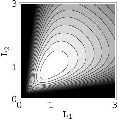
Figure 1: $\frac{24L_{\textrm{Y}}}{\pi}V_{1/L}(L_{1},L_{2},1)$ in $D=3$.

6 Lattice gauge theory

Numerical simulations of lattice gauge theory were performed in $D=3$. $V_{{\textrm{q}}{\textrm{q}}{\textrm{q}}}$ was extracted from Polyakov loop correlators using the method of Ref. [5] on a $48^{2}\times 32$ lattice with lattice spacing $a\approx 0.15\,\text{fm}$ ($\beta=11$), for one qqq geometry. The deviation from a pure Y law (with the measured mesonic string tension) is shown in Fig. 2.

Figure 2: $V_{{\textrm{q}}{\textrm{q}}{\textrm{q}}}-\sigma_{{\textrm{q}}\bar{\textrm{q}}}L_{\textrm{Y}}-c_{{\textrm{q}}\bar{\textrm{q}}}$ from lattice simulations for rectangular, isosceles qqq geometries with either the large side or the small sides of the triangle aligned with lattice axes. The curves are fits $c-b/L_{\textrm{Y}}$.The Y law is approached from above.

The asymptotic Y law is clearly approached from above as predicted, making the potential non-concave, but the magnitude of the $1/L$ term appears too large: $V_{1/L}=1.2(2)\frac{\pi}{24L_{\textrm{Y}}}$ compared to a coefficient of $0.39$ as predicted by Eq. (5). The discrepancy may be due to the small quark separations: even for the largest geometries, the shortest string in the classical configuration is only $0.45\,\text{fm}$ long, so the string picture is hardly applicable. In addition, it should be noted that the numerical result is very sensitive to the estimate of the mesonic string tension. Finally, a mandatory extrapolation to $T\to\infty$ has not been performed yet, so that excited-state contributions may significantly affect the measured coefficient.

A more thorough check of the string predictions should also include other geometries. Finally, it would be very interesting to extend the calculation to larger $\text{SU}(N)$ gauge groups and compare with predictions from $1/N$ expansions.

References

[1]
C. Alexandrou, Ph. de Forcrand and A. Tsapalis,
Phys. Rev. D 65 (2002) 054503;
C. Alexandrou, Ph. de Forcrand and O. Jahn,
Nucl. Phys. Proc. Suppl. 119 (2002) 649.
[2]
T. T. Takahashi, H. Matsufuru, Y. Nemoto and H. Suganuma,
Phys. Rev. Lett. 86 (2001) 18;
Phys. Rev. D 65 (2002) 114509.
[3] M. Lüscher, K. Symanzik, P. Weisz,
Nucl. Phys. B 173 (1980) 365.