Searching for KvBLL calorons in $SU(3)$ lattice gauge field ensembles
${}^{\;}$ HU-EP-03/65

Abstract

We discuss Kraan - van Baal - Lee - Lu (KvBLL) solutions of the classical Yang-Mills equations with temperature in the context of $SU(3)$ lattice gauge theory. We present discretized lattice versions of KvBLL solutions and other dyonic structures, obtained by cooling in order to understand their variety and signature. An analysis of the zero modes of the lattice Dirac operator for different fermionic boundary conditions gives clear evidence for a KvBLL-like background of finite $T$ lattice subensembles with $Q=\pm 1$. Using APE-smearing we are able to study the topological charge density $q(x)$ of the configurations and to corroborate this interpretation.

1 INTRODUCTION AND RETROSPECT TO $SU(2)$

The discovery of new caloron solutions with non-trivial holonomy [1] has revived hopes for a semiclassical description of Yang-Mills theory at $T\neq 0$, in particular of the deconfinement transition. A new aspect of these solutions is the interplay between topological charge and the local and asymptotic Polyakov loop. One new feature, the separation of a $Q=1$ object (caloron) into $N_{c}$ dyonic ($D$) constituents, happens only in some part of the parameter space which seems to be statistically enhanced in the confinement phase.

For a couple of years some of us have been searching [2] for this type of semiclassical background in $SU(2)$ lattice Monte Carlo configurations at finite $T$, mostly using cooling. Besides of opening a zoo of possible lattice solutions, a remarkable outcome was that, near $T_{c}$, the confinement phase is distinguished from deconfinement by a finite yield of non-trivial caloron configurations with 2 dyonic constituents. Sometimes they are separated into peaks of action, identifiable also by different localizations of the fermionic zero mode for periodic/antiperiodic temporal b.c., but always monopole pairs can be seen inside, such that the Polyakov loop $P(x)$ changes from $+1$ to $-1$. Somewhat unexpectedly, also $D\bar{D}$ pairs have been obtained by cooling as metastable solutions, with action $S\approx S_{inst}$ and equal-sign Polyakov loop. This happens only in the confined phase where the $D\bar{D}$ pairs originate from caloron-anti-caloron structures. Recently we have repeated the $SU(2)$ cooling studies at lower temperature. We found now that all calorons consist of overlapping action lumps, yet the Polyakov loop exhibits their non-trivial caloron nature.

2 SIGNATURE OF $SU(3)$ CALORONS

Let us now come to $SU(3)$. We parametrize as ${\cal P}_{\infty}=\mathrm{diag}(\mathrm{e}^{2\pi i\mu_{1}},\mathrm{e}^{2\pi i\mu_{2}},\mathrm{e}^{2\pi i\mu_{3}})$ the asymptotic holonomy, with $\mu_{1}\leq\mu_{2}\leq\mu_{3}\leq\mu_{4}=1+\mu_{1}$ and $\mu_{1}+\mu_{2}+\mu_{3}=0$. Let $\vec{y}_{1}$, $\vec{y}_{2}$ and $\vec{y}_{3}$ be three $3D$ position vectors remote from each other. Then a KvBLL [1] caloron consists of 3 lumps carrying the instanton action split into fractions $\mu_{2}-\mu_{1}$, $\mu_{3}-\mu_{2}$ and $\mu_{4}-\mu_{3}$, concentrated near the $\vec{y}_{i}$.

We discretized continuum calorons and applied a few cooling iterations to adapt it to torus boundary condition for the gauge field. Then an action $S\approx 1.3S_{inst}$ and a topological charge $Q=\pm 1$ are found. In Fig. 1 we show two extreme cases of lattice KvBLL solutions with well separated positions $\vec{y}_{i}$: a non-trivial one with almost equidistant phases $\mu_{i}$ and a caloron of trivial holonomy, i.e., ${\cal P}_{\infty}\approx\mathrm{diag}(1,1,1)$, $\mu_{1},\mu_{2},\mu_{3}\approx 0$. In the trivial case one of the constituents carries (almost) all action and topological charge.

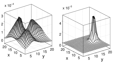
Figure 1: Topological charge density in the plane through all 3 constituent positions for a nontrivial (l.h.s.) and a trivial (r.h.s) KvBLL caloron.

In Ref. [3] the zero mode $\psi_{0}$ of the Dirac operator in the background of a KvBLL solution was analytically computed, introducing an arbitrary phase in the temporal b.c. of the Dirac operator, i.e., $\psi_{0}(t+1/T,\vec{x})=\exp(2\pi i\zeta)\,\psi_{0}(t,\vec{x})$. An intricate interplay between the phase parameter $\zeta$ and the holonomy phases $\mu_{i}$ was found. The zero mode is not localized simultaneously at all dyonic constituents. Instead, it chooses one of them and changes its position with changing value of $\zeta$. A selection rule states that the zero mode is localized at the position $\vec{y}_{i}$ of the $i$-th constituent if $\mu_{i}\leq\zeta\leq\mu_{i+1}$. This implies that for a set of well-separated $\mu_{i}$ and $\vec{y}_{i}$ the zero mode will visit all 3 constituents during one cycle of $\zeta$ from 0 to 1. 

We demonstrate this effect using the chirally improved lattice Dirac operator [4]. This operator has good chiral properties and is known to reproduce the zero mode of latticized standard instantons [5]. We clearly reproduce the behavior of the zero mode for the non-trivial caloron (see Fig. 2). We plot the scalar density of the zero mode. This gauge invariant observable is obtained by summing $|\psi_{0}(x)|^{2}$ at each lattice point $x$ over color and Dirac indices. In order to assess the physical relevance of calorons, one should study the correlation between the zero mode positions and the topological charge density $q(x)$ and find out the statistical distribution in the caloron parameter space. This could be difficult because generic equilibrium configurations might contain dyonic constituents difficult to separate. Yet it is indispensable because the calorons have to be disentangled from the additional topological structure which might be of different nature.

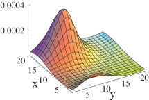
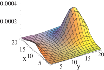
Figure 2: Scalar density for the non-trivial KvBLL caloron of Fig. 1. We show 2 zero modes obtained with $\zeta=0.5$ (l.h.s.) and $\zeta=0.8$ (r.h.s.).

3 COOLED CALORONS AND OTHER OBJECTS

In order to explore the appearance of more general $SU(3)$ KvBLL solutions on the lattice we cooled hot configurations in the confinement phase on $16^{3}\times 4$ lattices (created with Wilson gauge action at $\beta=5.5$), keeping torus b.c. for the gauge field. Then the evolution of the holonomy, starting from an average Polyakov loop $\bar{P}\approx 0$ (where $P=\frac{1}{3}\mbox{tr}{\cal P}$), is not predictable. With increasing number of cooling steps $n_{cool}$ the asymptotic Polyakov loop $\bar{P}_{\infty}$ (an average over all lattice points where the local action density $s<10^{-4}$) becomes more and more scattered over the complex region accessible for the Polyakov loop. One can find cooled configurations with any non-trivial holonomy. Quasiclassical lattice configurations are identified when the cooling history $S(n_{cool})$ goes through a plateau i.e., the equations of motion are minimally violated. The distribution in $\bar{P}_{\infty}$ is more centered around the origin for higher plateaus and more spread for the caloron plateaus $S=S_{inst}$. Of course, only part of the caloron events with asymptotic holonomy $\bar{P}_{\infty}\notin Z(3)$ have such a clean $DDD$ structure of the action density as the non-trivial example shown in Fig. 1. Most of the $S=S_{inst}$ plateaus have only two distinguishable lumps of action. Nevertheless, all caloron events are characterized by a distribution of the Polyakov loop field $P(\vec{x})$ as shown in Fig. 3 where the ideal non-trivial caloron is compared with a generic caloron (two-lump) event. The bulk of lattice points represents the asymptotic holonomy while the constituents are mapped to the envelope of this plot. In the metric of $P$, the distance of a constituent from the bulk is proportional to the fraction of action (topological charge) it carries.

Purely (anti-)selfdual configurations are most frequently observed on the $S=S_{inst}$ and $S=2S_{inst}$ plateaus. The latter, analogous to the calorons, preferentially contain four lumps of action, but probably belong to a wider class of $Q=\pm 2$ KvBLL solutions. Besides of these, we have found metastable cooled configurations which are not of KvBLL caloron type. In the $Q=0$ sector we found $D\bar{D}$ events at plateaus $S\approx 0.65S_{inst}$ as well as $DD\bar{D}\bar{D}$ events at $S\approx 1.35S_{inst}$, usually left over from the annihilation of $D$’s and $\bar{D}$’s, former constituents of caloron and anti-caloron in a confinement configuration.

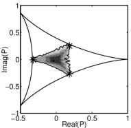
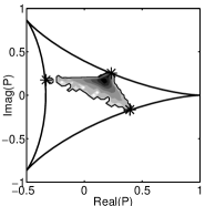
Figure 3: Polyakov loop distributions over the volume for the constructed non-trivial caloron of Fig. 1 (l.h.s) and for a caloron obtained by cooling (r.h.s.). Constituents are marked with stars.

4 ZERO MODES FOR $Q=\pm 1$ EQUILIBRIUM CONFIGURATIONS

In the last few years it was understood that the low lying eigenmodes of the lattice Dirac operator provide a good filter which removes short distance fluctuations of the gauge field allowing the study of topological objects on the lattice. This mostly concerns the near zero modes. The peculiar behavior of the zero mode known for the KvBLL configurations suggests that this $\zeta$ dependence for any zero mode might be an excellent, simple and stable tool to highlight the presence of caloron background fields in equilibrium configurations among other carriers of topological charge, without cooling. A more detailed account of the results presented in this section can be found in Ref. [6].

We have computed eigenmodes of the chirally improved lattice Dirac operator [4], using quenched $SU(3)$ gauge ensembles generated with the Lüscher-Weisz action [7] on $20^{3}\times 6$ lattices at inverse gauge couplings of $\beta=8.20$ and $\beta=8.45$. These values correspond to lattice spacings of $a=0.115$ fm and $a=0.094$ fm and describe physics just below and above the QCD phase transition (located at $\beta_{c}=8.24$ [8]). From the full ensembles of gauge configurations we have selected those configurations which have only a single zero mode, i.e., configurations with topological charge $Q=\pm 1$. This choice leads one to consider only the simplest case where no mixing between different zero modes can occur. All or a certain fraction of these configurations might contain the excess topological charge $\pm 1$ in the form of well-separated dyons.

For an equilibrium configuration, let us illustrate the effect of changing fermionic b.c. on the scalar density of the zero mode $\psi_{0}$. In Fig. 4 we show $x$-$y$ slices of the scalar density of the zero mode for the configuration No. 125 from the confined ensemble and compare the cases of anti-periodic and periodic temporal fermionic boundary conditions. The position of the zero mode is seen to change under a switch from $\zeta=0$ to $\zeta=0.5$ which gives us 2 out of 3 expected locations. Later we will show that in all 3 positions the zero mode is located on top of lumps of topological charge with appropriate sign. In the particular example shown in Fig. 4 the two positions are 1.3 fm apart.

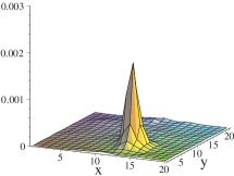
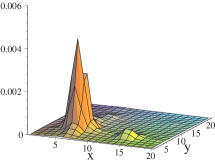
Figure 4: Scalar density of the zero mode of config. No. 125 (confined phase) for anti-periodic (l.h.s.) and periodic b.c. (r.h.s.). In each case we show the $x$-$y$ slice containing the maximum.

For a more systematical study we computed the zero mode 10 times on the same configuration using values of $\zeta=0.0,0.1,0.2,...,0.9$ in the fermionic b.c.. This detailed investigation was done for 10 configurations in the confined phase ($\beta=8.20$) and 10 configurations in the deconfined phase ($\beta=8.45$).

In the confined phase the expectation value of the Polyakov loop vanishes, suggesting a choice $\mu_{1}=-1/3$, $\mu_{2}=0$, $\mu_{3}=1/3$, $\mu_{4}=2/3$. The selection rule then implies that $\zeta$ can be contained in three different intervals $[0,1/3]$, $[1/3,2/3]$, $[2/3,1]$, each selecting another dyonic constituent. For 5 of our 10 configurations we found that the zero mode indeed visits exactly 3 different lumps. For 3 of the 10 configurations we found only 2 distinct lumps. The explanation might be that two of the constituents are very close to each other in space. Finally, for 2 of the 10 configurations we found even 4 different positions of the zero mode. This latter observation could be an effect of large quantum fluctuations on top of the infrared structure mimicking an additional peak. It would be interesting to repeat the calculation on a finer lattice with the same temperature where one expects the disturbance from quantum fluctuations to be less severe.

In the deconfined phase the Polyakov loop has a non-vanishing expectation value. Due to the center symmetry of the gauge action this expectation value can be realized with three different $Z(3)$ phases $0,\pm 2\pi/3$. For real Polyakov loop one has $\mu_{1}\approx\mu_{2}\approx\mu_{3}\approx 0$ and $\mu_{4}\approx 1$. Roughly speaking, the boundary phase parameter $\zeta$ can be contained only in the two intervals $[0,0]$ and $[0,1]$. Only for $\zeta\approx 0$ the zero mode is not able to see the same lump that it sees for all other $\zeta\neq 0$, which contains a well-localized topological charge ($Q\approx\pm 1$). For configurations with complex Polyakov loop (phase $\pm 2\pi/3$) this critical value of $\zeta$ is shifted to $1/3$ respectively $2/3$. Our set of 10 configurations in the deconfined phase contained configurations with real Polyakov loop as well as with complex Polyakov loop (here we also computed the values $\zeta=1/3,2/3$). For all 10 configurations we confirmed that only for the critical value of $\zeta$ a different position of the zero mode may be taken.

For a larger set of 89 deconfined configurations and 70 confined ones we followed the numerically cheaper approach of comparing only the periodic ($\zeta=0.0$) with the the anti-periodic ($\zeta=0.5$) zero mode. For both boundary conditions we determined the position of the corresponding peak and then computed the Euclidean distance $d_{4}$ between the two peaks. The histograms of distances are shown in Fig. 5. In the confinement phase (l.h.s.) $d_{4}$ is distributed over all distances. The histogram for deconfinement (r.h.s.) shows that for many configurations the mode does not jump at all or only over a small $d_{4}$. There is only a small, separate component in the histogram with $d_{4}\geq 9a$, all related to configurations having a real Polyakov loop $\bar{P}$. We highlight this subsample of the deconfined phase in the r.h.s. plot.

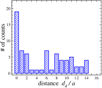
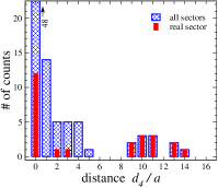
Figure 5: Histograms of the distance between the peak positions of the periodic and the anti-periodic zero mode in the confined (l.h.s) and deconfined phase (r.h.s.).

This observation confirms the selection rule for zero modes in a KvBLL background. It allows jumps between periodic and anti-periodic b.c. only in the real sector. This does, however, not imply that the zero mode in the real sector always jumps over large distances since the two constituents might be close to each other. In Ref. [6] several other tests of the zero modes were performed such as a study of their inverse participation ratio, a measure of their localization, as function of $\zeta$. Throughout we found fair agreement with the properties of zero modes in the background of a KvBLL solution in the confined phase and even excellent agreement in the case of the deconfined phase. We have also extended our study of zero modes with general boundary conditions to lattices with zero temperature geometry and still find jumping of the zero modes. A detailed writeup of these observations is in preparation.

In the meantime KvBLL solutions have been generalized to higher topological charge, and their corresponding zero modes have been constructed analytically [9]. It would be interesting to perform a study of the zero modes in higher topological sectors. We also remark that in Ref. [10] it was argued that the effect of jumping zero modes can hardly be due to overlapping standard instantons and therefore this effect is truly a consequence of the presence of a KvBLL background in the $Q=\pm 1$ configurations under study.

5 COMPARISON WITH SMOOTHING

We have experimented with cooling techniques in order to study the correlation between the topological charge density and the positions occupied by the zero mode with changing $\zeta$. We tried restricted cooling [11], adapted to the Lüscher-Weisz action, and APE smearing. The latter procedure was used by A. Hasenfratz et al. [12] to disclose the topological content of lattice fields. In the confinement phase the emerging structures are similar for both procedures (which therefore can be tuned to each other) and relatively stable with respect to cooling/smearing iterations.

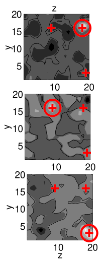
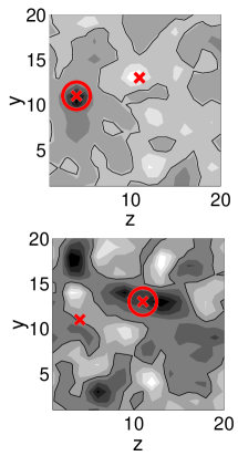
Figure 6: Topological charge density in $y$-$z$ planes, each through one of the zero mode positions (marked by the circle): confined config. No. 125 with 3 different localizations (l.h.s.) and deconfined config. No. 383 with 2 different localizations (r.h.s.).

Here we concentrate on results obtained by APE smearing with $N_{smear}=10$ iterations and $\alpha=0.45$ [12]. As an example for the confined phase we show configuration No. 125 on the l.h.s. of Fig. 6. The map of the topological density is shown in three $y$-$z$ slices, selected such that each contains one of the 3 zero mode positions. Crosses show the projection of all 3 positions on the given plane, while crosses with circles emphasize the zero mode sitting in the plane. There is a complex pattern of positive and negative charge density while the total charge is $Q=-1$. The zero mode always settles at same-sign lumps which are all well-localized. The topological charge is not exactly balanced between the lumps, because the largest $\zeta$ interval corresponds to $t_{zm}=5$, $x_{zm}=14$, $y_{zm}=16$, $z_{zm}=18$ (the position in the upper plot).

As an example for the deconfined phase we show configuration No. 383 on the r.h.s. of Fig. 6. The configuration has $Q=1$ and a real-valued asymptotic Polyakov loop. For almost all $\zeta$ the zero mode is localized on top of the well-localized constituent seen in the upper plot. For $\zeta\approx 0$ however, the zero mode appears much less-localized in another region of topological density $q(x)>0$. The topological charge is much less concentrated there, too, consisting of two lumps with the zero mode center in between.

Obviously, also in the deconfined phase one finds a complex topological structure which is more sensitive to cooling than in the confinement phase. The gap separating the near zero modes strongly depends on it. We have observed that the gap rapidly closes if we cool too much.

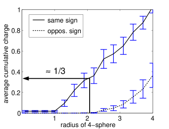
Figure 7: Cumulative topological charge of same sign and opposite sign as function of radius $R$ around the center of a zero mode (in the confined config. No. 125).

For the confined configuration No. 125 and for the three possible localizations of the zero mode we calculated the cumulative topological charges of same and opposite sign (relative to $Q$) as a function of the radius of a 4-sphere. The curves shown in Fig. 7 are an average over the three cases. The radius inside of which the topological density has a coherent sign of $q(x)$ is a good definition of the constituent radius. Then the average topological charge of a constituent is $Q_{const}\approx\pm\frac{1}{3}$ in the confinement phase.

6 CONCLUSIONS

We obtained new classical solutions by cooling of confined $SU(3)$ lattice configurations. For Monte Carlo configurations in the topological sector $Q=\pm 1$, the dependence of the localization of the fermionic zero mode on the aperiodicity angle $\zeta$ matches the specific expectations derived from the KvBLL caloron picture for the confined and deconfined phases. For slightly APE-smeared configurations we are able to corroborate these findings by considering the topological charge distribution close to the zero mode locations.

References

- [1] T.C. Kraan and P. van Baal, Phys. Lett. B 428 (1998) 268, ibid. B 435 (1998) 389, Nucl. Phys. B 533 (1998) 627; K. Lee and C. Lu, Phys. Rev. D 58 (1998) 1025011.
- [2] E.-M. Ilgenfritz, B. V. Martemyanov, M. Müller-Preussker, S. Shcheredin and A. I. Veselov, Phys. Rev. D 66 (2002) 074503.
- [3] M. Garcia Pérez, A. González-Arroyo, C. Pena and P. van Baal, Phys. Rev. D 60 (1999) 031901; M.N. Chernodub, T.C. Kraan and P. van Baal, Nucl. Phys. Proc. Suppl. 83 (2000) 556.
- [4] C. Gattringer, Phys. Rev. D 63 (2001) 114501; C. Gattringer, I. Hip and C.B. Lang, Nucl. Phys. B 597 (2001) 451.
- [5] C. Gattringer et al. Phys. Lett. B 522 (2001) 194.
- [6] C. Gattringer, Phys. Rev. D 67 (2003) 034507; C. Gattringer and S. Schaefer, Nucl. Phys. B 654 (2003) 30.
- [7] M. Lüscher and P. Weisz, Commun. Math. Phys. 97 (1985) 59.
- [8] C. Gattringer, R. Hoffmann and S. Schaefer, Phys. Rev. D 65 (2002) 094503; C. Gattringer, P.E.L. Rakow, A. Schäfer and W. Söldner, Phys. Rev. D 66 (2002) 054502.
- [9] F. Bruckmann and P. van Baal, Nucl. Phys. B 645 (2002) 105; F. Bruckmann, D. Nogradi and P. van Baal, hep-th/0305063.
- [10] F. Bruckmann, M. Garcia Pérez, D. Nogradi and P. van Baal, hep-lat/0308017.
- [11] M. Garcia Pérez, O. Philipsen and I. O. Stamatescu, Nucl. Phys. B 551 (1999) 293.
- [12] T. DeGrand, A. Hasenfratz and T. G. Kovacs, Nucl. Phys. B 520 (1998) 301; A. Hasenfratz and C. Nieter, Phys. Lett. B 439 (1998) 366.