Recent Developments in Lattice Supersymmetry

Abstract

I discuss a new approach to constructing lattices for gauge theories with extended supersymmetry. The lattice theories themselves respect certain supersymmetries, which in many cases allows the target theory to be obtained in the continuum limit without fine-tuning.

1 Introduction

Supersymmetric gauge theories are known to exhibit diverse fascinating phenomena (See, for example, [1, 2, 3]). These include phenomena seen in QCD, such as confinement and chiral symmetry breaking. In some cases one can demonstrate phenomena suspected to be important in QCD, such as magnetic monopole condensation and instantons. Others exhibit phenomena which are decidedly unlike QCD, such as massless composite fermions. There exist pairs of theories which have quite different Lagrangian descriptions (such as different gauge groups) which are believed to be dual to each other. Some of these theories are expected to possess nontrivial conformal fixed points in the infrared. A particularly special case, ${\cal N}=4$ supersymmetric Yang-Mills theory (SYM) in four dimensions is thought to be exactly conformal and to be self-dual. Understanding these theories in detail would greatly expand our knowledge of field theory. These theories could be of more than pedagogical importance however. Many have speculated that strongly coupled SYM theories could explain the hierarchy between the weak and GUT scales and the baffling pattern of quark and lepton masses. Beyond that, string theory and all of quantum gravity is thought to be related to such theories in the large-$N_{c}$ limit, where $N_{c}$ is the number of colors of the gauge group.

Up until recently there has not existed a non-perturbative regulator for such theories, and so our knowledge of their behavior has been limited to certain analytical calculations and informed speculation.

Recently there have been a number of interesting developments in lattice supersymmetry, such as work on the $d=2$ dimensional Wess-Zumino model [4, 5, 6, 7], on $d=4$, ${\cal N}=1$ SYM theory [8, 9, 10], as well as other supersymmetric theories [11, 12, 13]. In this talk I will tell you about recent progress I have made with my collaborators A. Cohen, E. Katz, and M. Ünsal in constructing lattice theories whose continuum limits are various SYM theories in various dimensions [14, 15, 16, 17]. In many cases we can show that the target theory is obtained in the continuum limit without the need for fine-tuning of couplings. This is accomplished by maintaining some unbroken supersymmetry at finite lattice spacing, an approach shared by the recent work discussed at this conference by Simon Catterall [4, 11]. The lattices that result are quite unlike ones that are usually considered by lattice theorists. I intend to exhibit some of their peculiar and almost magical properties, such as the emergence of chiral symmetries in the continuum without having to resort to overlap or domain wall fermions.

2 Accidental Supersymmetry

Formulating a supersymmetric lattice gauge theory is difficult, since supersymmetry is actually an extension of the Poincaré algebra, which is explicitly broken by the lattice. In particular, the central feature of the super-Poincaré algebra is the anti-commutator of a supercharge $Q_{\alpha}$ and its conjugate $\kern 0.6pt\overline{\kern-0.6ptQ\kern-0.6pt}\kern 0.6pt_{\dot{\alpha}}$, which yields the generator of infinitesimal translations, $P_{\mu}$. Schematically, $\{Q,\kern 0.6pt\overline{\kern-0.6ptQ\kern-0.6pt}\kern 0.6pt\}\sim 2P$. On the lattice there are no infinitesimal translations, and therefore the supersymmetry algebra must be broken.

Nevertheless, we are quite familiar with the continuum limit of a lattice theory possessing more symmetry than the lattice action itself, and we might hope to construct non-supersymmetric lattices with supersymmetric continuum limits. Certainly it ought to be possible to accomplish with enough fine-tuning of coupling constants, but that approach is neither feasible in practice nor theoretically satisfying. An obvious paradigm to emulate is the emergence of Poincaré symmetry without fine-tuning in lattice QCD. The way this works is that the exact symmetries of the lattice theory — specifically gauge symmetry and the hypercubic crystal symmetry — forbid operators with dimension $\leq 4$ which violate Poincaré symmetry. Thus at weak coupling, the theory flows to a Poincaré symmetric point in the infrared without any fine-tuning of couplings required. In this sense, Poincaré symmetry emerges as an “accidental” symmetry in the continuum. As we well know, one is not always so lucky: witness the difficulties in obtaining chiral symmetry in the continuum limit of lattice QCD.

Although we cannot construct lattices which obey the super-Poincaré algebra, we may still hope to find lattices for which supersymmetry emerges as an accidental symmetry in the infrared.

A simple example of a non-supersymmetric theory with a supersymmetric limit in the infrared is an $SU(N)$ gauge theory with a single Weyl spinor transforming in the adjoint representation, respecting an exact $Z_{2N}$ chiral symmetry, the anomaly-free subgroup of phase rotations of the fermion. Such a theory has ${\cal N}=1$ SYM as its infrared limit, since the only possible supersymmetry violating relevant operator allowed by the gauge and spacetime symmetries is a fermion mass, and that is forbidden by the anomaly-free $Z_{2N}$ chiral symmetry [18]. It is possible to construct such a theory on the lattice using overlap or domain wall fermions [19, 20, 21, 22]. It is also possible to dispense with the chiral symmetry and to use Wilson fermions, making one fine-tuning (setting the fermion mass to zero) in order to obtain the supersymmetric target theory [8]. This is a very interesting theory to study, but as it requires dynamical fermions to exhibit supersymmetry, the technical challenges to simulating the theory are great.

In four dimensions, the above example of pure ${\cal N}=1$ SYM theory is the only supersymmetric theory without scalar fields. If one wishes to simulate any other supersymmetric theory in $d=4$ dimensions, then scalars must be introduced, and the situation looks grim. That is because among the plethora of relevant supersymmetry violating operators that must now be considered, one is a mass term for the scalar. There are only two symmetries which can forbid a scalar mass term. The first is a shift symmetry, $\phi\to\phi+f$, where $f$ is a constant. This results in $\phi$ only having derivative interactions…it is a Goldstone boson. Such a theory cannot describe most supersymmetric theories of interest, including SYM theories, in which scalar fields have gauge interactions.

The second symmetry which can forbid mass terms is supersymmetry. This reasoning seems to have led us in full circle: due to the difficulties in realizing supersymmetry exactly on the lattice, we are led to look for non-supersymmetric theories exhibiting accidental supersymmetry; but accidental supersymmetry seems to require exact supersymmetry in order to forbid scalar mass terms.

All that remains to us is a sort of compromise: perhaps we can construct a lattice with a little bit of exact supersymmetry, enough to forbid relevant operators which violate any of the target theories more extensive supersymmetry. There are lots of reasons to expect this approach to fail for SYM theories, however:

$\bullet$ Presumably the exact supersymmetry would require scalar, fermions and gauge fields to exist in the same multiplet. But then if gauge fields live on links, one would expect their supersymmetric partners to as well. But how can spin zero bosons reside on links, which would require them to transform nontrivial under the exact lattice rotations, and hence (one would expect) under continuum Lorentz transformations?

$\bullet$ With so many particles of different spin around, it would seem difficult to even realize accidental Lorentz symmetry in the continuum due to the large number of relevant Lorentz violating interactions. Lorentz violation has been the outcome of many attempts to construct lattices with partial supersymmetry, such as in ref. [23];

$\bullet$ The SYM target theories typically have large chiral symmetries (called $R$-symmetries) which do not commute with the supersymmetry. For example, ${\cal N}=4$ supersymmetry in $d=4$ has an $SU(4)$ $R$-symmetry, under which the fermions transform as the four dimensional defining representation, while the scalars transform as the six dimensional antisymmetric tensor. Our experience with lattice QCD suggests that we would either have to fine-tune the theory to realize these symmetries, or else employ overlap or domain wall fermions. In the latter cases it is hard to imagine how there could be a supersymmetry relating such fermions to scalars or gauge bosons, which have quite different implementations.

Happily, we have found that there exist lattices which get around all of the above objections. The technical details of how to construct these lattices are given in refs. [14, 15, 16, 17]; here I will focus instead on what the lattices look like, and how they work. I will begin by discussing a lattice theory for SYM in two Euclidean dimensions, possessing four real supercharges.

(A matter of nomenclature: rather than designating the amount of supersymmetry by ${\cal N}=1$, ${\cal N}=2$, etc. in dimensions $d<4$, which gets confusing, I will instead refer to the number of real supercharges ${\cal Q}$. For comparison, ${\cal N}=1$, ${\cal N}=2$ and ${\cal N}=4$ SYM theories in $d=4$ possess ${\cal Q}=4$, ${\cal Q}=8$ and ${\cal Q}=16$ real supercharges respectively.)

3 Super Yang Mills in $d=2$ with ${\cal Q}=4$

This target theory is just what one gets upon reducing conventional ${\cal N}=1$ SYM theory in $d=4$ down to $d=2$. The particle content is a two component gauge field $v_{m}$, one complex scalar $s$, and a Dirac fermion $\psi$. All of these fields transform as adjoints under the gauge symmetry. The Lagrangean in Euclidean space is given by

$${\cal L} =\frac{1}{g_{2}^{2}}\,{\rm Tr}\,\Biggl{(}\bigl{|}D_{m}s\bigr{|}^{2}+\kern 0.6pt\overline{\kern-0.6pt\psi\kern-0.6pt}\kern 0.6pt\,D_{m}\gamma_{m}\psi+{\textstyle{\frac{1}{4}}}v_{mn}v_{mn}$$ (1)

$$+\sqrt{2}(\kern 0.6pt\overline{\kern-0.6pt\psi\kern-0.6pt}\kern 0.6pt_{L}[s,\psi_{R}]+\kern 0.6pt\overline{\kern-0.6pt\psi\kern-0.6pt}\kern 0.6pt_{R}[s^{\dagger},\psi_{L}])-{\textstyle{\frac{1}{2}}}[s^{\dagger},s\,]^{2}\Biggr{)}$$

In the above equation, $v_{mn}$ is the gauge field strength, and $g_{2}$ is the gauge coupling. Note that this theory exhibits an anomalous chiral $U(1)$ symmetry, involving both $\psi$ and $s$.

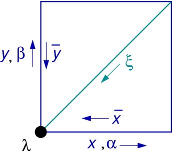
Figure 1: The lattice for SYM in $d=2$ with ${\cal Q}=4$ supercharges. Latin letters correspond to one-component complex bosons, Greek letters to one component fermions.

Our lattice for this theory has the structure shown in Fig. 1. It consists of two complex bosons $x$ and $y$, and four one-component Grassmann variables $\alpha$, $\beta$, $\lambda$ and $\xi$. All fields are $k\times k$ matrices At each site there is an independent $U(k)$ symmetry, which will become a $U(k)$ gauge symmetry in the continuum; $\lambda$ transforms as a $U(k)$ adjoint, while the link variables are bifundamentals $(\,\raisebox{-0.5pt}{\hbox{\rule{0.4pt}{6.5pt}\hskip-0.4pt\rule{6.5pt}{0.4pt}\hskip-6.5pt\rule[6.5pt]{6.5pt}{0.4pt}}\rule[6.5pt]{0.4pt}{0.4pt}\hskip-0.4pt\rule{0.4pt}{6.5pt}}\,,\kern 0.6pt\overline{\kern-0.6pt\raisebox{-0.5pt}{\hbox{\rule{0.4pt}{6.5pt}\hskip-0.4pt\rule{6.5pt}{0.4pt}\hskip-6.5pt\rule[6.5pt]{6.5pt}{0.4pt}}\rule[6.5pt]{0.4pt}{0.4pt}\hskip-0.4pt\rule{0.4pt}{6.5pt}}\kern-0.6pt}\kern 0.6pt\,)$ or the conjugate, depending on the orientation of the arrows shown in the figure.

3.1 The lattice action and its classical limit

The lattice action is given by

$$\frac{1}{g^{2}}\sum_{\mathbf{n}}{\rm Tr}\,\Bigl{[} {\textstyle{\frac{1}{2}}}\left(\kern 0.6pt\overline{\kern-0.6ptx\kern-0.6pt}\kern 0.6pt_{\mathbf{n}-\mathbf{\hat{e}}_{1}}x_{\mathbf{n}-\mathbf{\hat{e}}_{1}}-x_{\mathbf{n}}\kern 0.6pt\overline{\kern-0.6ptx\kern-0.6pt}\kern 0.6pt_{\mathbf{n}}\right.\Bigr{.}$$ (2)

$$+\left.\kern 0.6pt\overline{\kern-0.6pty\kern-0.6pt}\kern 0.6pt_{\mathbf{n}-\mathbf{\hat{e}}_{2}}y_{\mathbf{n}-\mathbf{\hat{e}}_{2}}-y_{\mathbf{n}}\kern 0.6pt\overline{\kern-0.6pty\kern-0.6pt}\kern 0.6pt_{\mathbf{n}}\right)^{2}$$

$$+2\,\bigl{|}x_{\mathbf{n}}y_{\mathbf{n}+\mathbf{\hat{e}}_{1}}-y_{\mathbf{n}}x_{\mathbf{n}+\mathbf{\hat{e}}_{2}}\bigr{|}^{2}$$

. $$+\sqrt{2}\,\left(\Delta_{{\bf n}}(\lambda,\kern 0.6pt\overline{\kern-0.6ptx\kern-0.6pt}\kern 0.6pt,\alpha)+\Delta_{{\bf n}}(\lambda,\kern 0.6pt\overline{\kern-0.6pty\kern-0.6pt}\kern 0.6pt,\beta)\right.$$

$$\left.-\Delta_{{\bf n}}(\xi,y,\alpha)+\Delta_{{\bf n}}(\xi,x,\beta)\right)\Bigr{]}$$

where ${\mathbf{n}}$ denotes the lattice position, $\mathbf{\hat{e}}_{1}$ and $\mathbf{\hat{e}}_{2}$ are unit lattice vectors, and

$$\Delta_{{\bf n}}(\lambda,\kern 0.6pt\overline{\kern-0.6ptx\kern-0.6pt}\kern 0.6pt,\alpha) =\lambda_{\bf n}\left(\kern 0.6pt\overline{\kern-0.6ptx\kern-0.6pt}\kern 0.6pt_{{\bf n}-\mathbf{\hat{e}}_{1}}\alpha_{{\bf n}-\mathbf{\hat{e}}_{1}}-\alpha_{\bf n}\kern 0.6pt\overline{\kern-0.6ptx\kern-0.6pt}\kern 0.6pt_{\bf n}\right)\ ,$$ (3)

$$\Delta_{{\bf n}}(\lambda,\kern 0.6pt\overline{\kern-0.6pty\kern-0.6pt}\kern 0.6pt,\beta) =\lambda_{\bf n}\left(\kern 0.6pt\overline{\kern-0.6pty\kern-0.6pt}\kern 0.6pt_{{\bf n}-\mathbf{\hat{e}}_{2}}\beta_{{\bf n}-\mathbf{\hat{e}}_{2}}-\beta_{\bf n}\kern 0.6pt\overline{\kern-0.6pty\kern-0.6pt}\kern 0.6pt_{\bf n}\right)\ ,$$

$$\Delta_{{\bf n}}(\xi,y,\alpha) =\xi_{\bf n}\left(y_{\bf n}\alpha_{{\bf n}+\mathbf{\hat{e}}_{2}}-\alpha_{\bf n}y_{{\bf n}+\mathbf{\hat{e}}_{1}}\right),$$

$$\Delta_{{\bf n}}(\xi,x,\beta) =\xi_{\bf n}\left(x_{\bf n}\beta_{{\bf n}+\mathbf{\hat{e}}_{2}}-\beta_{\bf n}x_{{\bf n}+\mathbf{\hat{e}}_{2}}\right)$$

(In fact I will need to add some more terms to the above action, as discussed below in §3.3.) As it stands, this “lattice” action looks bizarre: there are no hopping terms and no lattice spacing defined. The action has “classical flat directions”, or moduli. We will choose to expand the action about one particular point in this moduli space, namely

$$\langle x\rangle=\langle\kern 0.6pt\overline{\kern-0.6ptx\kern-0.6pt}\kern 0.6pt\rangle=\langle y\rangle=\langle\kern 0.6pt\overline{\kern-0.6pty\kern-0.6pt}\kern 0.6pt\rangle=\frac{1}{\sqrt{2}\,{a}}\,\times{\boldsymbol{1_{k}}}\ .$$ (4)

Here $\boldsymbol{1_{k}}$ is the $k$-dimensional unit matrix, and ${a}$ will soon be interpreted as the lattice spacing.

First, consider the bosonic part of the action. I rewrite the bosonic variables as

$$x\equiv\frac{1}{\sqrt{2}\,a}+\frac{s_{1}+iv_{1}}{\sqrt{2}}\ ,\quad y\equiv\frac{1}{\sqrt{2}\,a}+\frac{s_{2}+iv_{2}}{\sqrt{2}}\$$ (5)

and expand in powers of $a$. For example, $\kern 0.6pt\overline{\kern-0.6ptx\kern-0.6pt}\kern 0.6pt_{\mathbf{n}-\mathbf{\hat{e}}_{1}}x_{\mathbf{n}-\mathbf{\hat{e}}_{1}}-x_{\mathbf{n}}\kern 0.6pt\overline{\kern-0.6ptx\kern-0.6pt}\kern 0.6pt_{\mathbf{n}}$ is expanded as

$$\left(\frac{1}{\sqrt{2}\,a}+\frac{s_{1}-iv_{1}}{\sqrt{2}}-a\frac{\partial\ }{\partial x}\frac{s_{1}-iv_{1}}{\sqrt{2}}+O(a^{2})\right)$$

$$\times \left(\frac{1}{\sqrt{2}\,a}+\frac{s_{1}+iv_{1}}{\sqrt{2}}-a\frac{\partial\ }{\partial x}\frac{s_{1}+iv_{1}}{\sqrt{2}}+O(a^{2})\right)$$

$$- \left(\frac{1}{\sqrt{2}\,a}+\frac{s_{1}+iv_{1}}{\sqrt{2}}\right)\times\left(\frac{1}{\sqrt{2}\,a}+\frac{s_{1}-iv_{1}}{\sqrt{2}}\right)$$

$$= -i[v_{1},s_{1}]-\frac{\partial s_{1}}{\partial x}+O(a)$$

$$= -D_{1}s_{1}+O(a)\ ,$$

with $D_{m}=\partial_{m}+i[v_{m},\cdot]$. Note that while naively the expression $(\kern 0.6pt\overline{\kern-0.6ptx\kern-0.6pt}\kern 0.6pt_{\mathbf{n}-\mathbf{\hat{e}}_{1}}x_{\mathbf{n}-\mathbf{\hat{e}}_{1}}-x_{\mathbf{n}}\kern 0.6pt\overline{\kern-0.6ptx\kern-0.6pt}\kern 0.6pt_{\mathbf{n}})$ looks to be $O(a^{-2})$, it is in fact finite as $a\to 0$ due to its commutator-like structure.

Carrying out this expansion in powers of $a$ of the various terms in the lattice action Eq. (2) I find

$$\frac{1}{g^{2}}\sum_{\mathbf{n}}{\rm Tr}\,\Bigl{[}{\textstyle{\frac{1}{2}}}\left(\kern 0.6pt\overline{\kern-0.6ptx\kern-0.6pt}\kern 0.6pt_{\mathbf{n}-\mathbf{\hat{e}}_{1}}x_{\mathbf{n}-\mathbf{\hat{e}}_{1}}-x_{\mathbf{n}}\kern 0.6pt\overline{\kern-0.6ptx\kern-0.6pt}\kern 0.6pt_{\mathbf{n}}\right.$$ (6)

$$\qquad\qquad+\left.\kern 0.6pt\overline{\kern-0.6pty\kern-0.6pt}\kern 0.6pt_{\mathbf{n}-\mathbf{\hat{e}}_{2}}y_{\mathbf{n}-\mathbf{\hat{e}}_{2}}-y_{\mathbf{n}}\kern 0.6pt\overline{\kern-0.6pty\kern-0.6pt}\kern 0.6pt_{\mathbf{n}}\right)^{2}\Bigr{]}$$

$$=\ \ \frac{1}{g^{2}a^{2}}\int d^{2}z\frac{1}{2}{\rm Tr}\,\left(D_{1}s_{1}+D_{2}s_{2}\right)^{2}+O(a)\ ,$$

and

$$\quad\frac{1}{g^{2}}\sum_{\mathbf{n}}2\,{\rm Tr}\,\bigl{|}x_{\mathbf{n}}y_{\mathbf{n}+\mathbf{\hat{e}}_{1}}-y_{\mathbf{n}}x_{\mathbf{n}+\mathbf{\hat{e}}_{2}}\bigr{|}^{2}$$ (7)

$$=\ \ \frac{1}{g^{2}a^{2}}\int d^{2}z\ \frac{1}{2}\left(D_{1}s_{2}-D_{2}s_{1}\right)^{2}+\frac{1}{4}[s_{1},s_{2}]^{2}$$

$$\qquad\qquad\qquad\qquad+\frac{1}{2}\left(v_{12}\right)^{2}+O(a)\ ,$$

with the field strength defined as $v_{mn}=-i[D_{m},D_{n}]$.

Note that the two terms Eq. (6) and Eq. (7) each individually violate the Euclidean rotation symmetry, but when added together they yield

$$\frac{1}{g^{2}a^{2}}\int d^{2}z\ \frac{1}{2}|D_{m}s|^{2}-\frac{1}{2}[s^{\dagger},s]^{2}+\frac{1}{4}v_{mn}v_{mn}+O(a),$$ (8)

with $s\equiv(s_{1}+is_{2})/\sqrt{2}$. This is identical to the bosonic action of the the target theory Eq. (1). Note that even though $\{x,y\}$ transform non-trivially under the discrete $C_{2v}$ symmetry of the lattice in Fig. 1, we see that the leading term in our expansion in powers of $a$ is invariant under rotations, with $v_{m}$ and $D_{m}$ transforming as 2-vectors and $s$ as a scalar — even though $s$ is constructed out of the real parts of $x$ and $y$, while the gauge fields are constructed out of the imaginary parts of $x$ and $y$. Even better, the action Eq. (8) exhibits an internal $U(1)$ symmetry consisting of phase rotations of $s$. This symmetry is just the $U(1)_{R}$ symmetry of the target theory; it does not exist as a symmetry in the lattice action. This bizarre and delightful behavior is characteristic of the supersymmetric lattices I will present here.

To expand the fermionic part of the lattice action Eq. (2) in powers of $a$, I define the spinors

$$\psi=\begin{pmatrix}\lambda\cr\xi\end{pmatrix}\ ,\qquad\kern 0.6pt\overline{\kern-0.6pt\psi\kern-0.6pt}\kern 0.6pt=i\begin{pmatrix}\alpha&\beta\end{pmatrix}$$ (9)

and the $\gamma$ matrices

$$\gamma_{1}=\sigma_{3}\ ,\quad\gamma_{2}=\sigma_{1}\ ,\quad\gamma_{3}=\sigma_{2}\ .$$ (10)

After a little work one finds that the fermionic part of the lattice action Eq. (2) reproduces the fermionic part of the target theory’s action in Eq. (1), plus corrections of $O(a)$. The lattice theory has no fermion doubler modes, and the anomalous $U(1)_{R}$ symmetry emerges in the fermion sector as well at leading order in $a$, even though not present as a symmetry of the lattice action. And, of course, we know that by yielding the ${\cal Q}=4$ SYM theory in the continuum limit, somehow the full two dimensional super-Poincaré symmetry has emerged as well.

At least at the classical level then, one finds that the lattice theory, expanded about the values Eq. (4) yields the desired target theory in the limit

$$a\to 0\ ,\quad g\to\infty\ ,\quad g_{2}\equiv ag\ {\text{fixed}}.$$ (11)

At this point I have provided no reason to expect radiative corrections to respect the symmetries we have found at the classical level. For example, the two expressions in Eqs. (6,7) indicate that bosonic kinetic terms which do not respect two dimensional Lorentz invariance are allowed by the $C_{2v}$ symmetry of the lattice, and that the target theory only emerges if the two terms are added with precisely related coefficients. One might expect that this delicate balance is destroyed by quantum effects. In fact, this does not happen, and that is because the lattice action Eq. (2) possesses an exact supersymmetry that tames the radiative corrections.

3.2 Exact lattice supersymmetry and radiative corrections

In order to make explicit the supersymmetry of the lattice action Eq. (2), it is convenient to develop a lattice superfield notation, with the action of a supercharge $Q$ being translation along a Grassmann coordinate $\theta$: $Q=\frac{\partial\ }{\partial\theta}$. We can define superfields constructed out of our lattice variables (and a new auxiliary field $d$):

$$\hskip 21.68121pt\mathbf{X}_{\mathbf{n}} =x_{\mathbf{n}}+\sqrt{2}\,\theta\,\alpha_{\mathbf{n}}$$ (12)

$$\mathbf{Y}_{\mathbf{n}} =y_{\mathbf{n}}+\sqrt{2}\,\theta\,\beta_{\mathbf{n}}$$

$$\boldsymbol{\Lambda}_{\mathbf{n}} =\lambda_{\mathbf{n}}-\left(({\kern 0.6pt\overline{\kern-0.6ptx\kern-0.6pt}\kern 0.6pt}_{\mathbf{n}-\mathbf{\hat{e}}_{1}}x_{\mathbf{n}-\mathbf{\hat{e}}_{1}}-x_{\mathbf{n}}{\kern 0.6pt\overline{\kern-0.6ptx\kern-0.6pt}\kern 0.6pt}_{\mathbf{n}})\right.$$

$$\ \left.+({\kern 0.6pt\overline{\kern-0.6pty\kern-0.6pt}\kern 0.6pt}_{\mathbf{n}-\mathbf{\hat{e}}_{2}}y_{\mathbf{n}-\mathbf{\hat{e}}_{2}}-y_{\mathbf{n}}{\kern 0.6pt\overline{\kern-0.6pty\kern-0.6pt}\kern 0.6pt}_{\mathbf{n}})+id_{\mathbf{n}}\right)\,\theta$$

$$\boldsymbol{\Xi}_{\mathbf{n}} =\xi_{\mathbf{n}}+2\left({\kern 0.6pt\overline{\kern-0.6ptx\kern-0.6pt}\kern 0.6pt}_{\mathbf{n}+\mathbf{\hat{e}}_{1}}{\kern 0.6pt\overline{\kern-0.6pty\kern-0.6pt}\kern 0.6pt}_{\mathbf{n}}-{\kern 0.6pt\overline{\kern-0.6pty\kern-0.6pt}\kern 0.6pt}_{\mathbf{n}+\mathbf{\hat{e}}_{2}}{\kern 0.6pt\overline{\kern-0.6ptx\kern-0.6pt}\kern 0.6pt}_{\mathbf{n}}\right)\,\theta\ .$$

The structure of these superfields is revealing. We see that application of the supercharge $Q=\frac{\partial\ }{\partial\theta}$ transforms $x$ into $\alpha$ and $y$ into $\beta$, as one might expect from Fig. 1. However the site fermion $\lambda$ transforms into a combination of the link bosons $x$ and $y$, which after the expansion about $x=y=\frac{1}{\sqrt{2}\,a}$ is related to the hopping terms for the scalar $s$. The diagonal link fermion $\xi$ transforms into a combination of the link bosons related to the plaquette, which gives hopping terms for the gauge field $v_{m}$. In this devious way supersymmetry becomes entwined with translations in the continuum limit of our lattice: the supercharge $Q$ does not have a $\frac{\partial\ }{\partial x}$ in its definition, but the superfields it acts on are slightly nonlocal. Note that in spite of this non-locality, the supersymmetry transformations are all gauge covariant, since the superfields I have written down are gauge covariant.

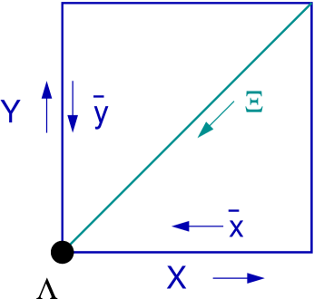
Figure 2: The lattice for SYM in $d=2$ with ${\cal Q}=4$ supercharges, in terms of the superfields of Eq. (12)

In terms of the superfields of Eq. (12) the lattice may be drawn as in Fig. 2. The lattice action Eq. (2) may be rewritten in terms of the superfields as

$$S= \frac{1}{g^{2}}\int\!d\theta\,\sum_{\mathbf{n}}{\rm Tr}\,\biggl{[}-{\textstyle{\frac{1}{2}}}\boldsymbol{\Lambda}_{\mathbf{n}}\,\partial_{\theta}\boldsymbol{\Lambda}_{\mathbf{n}}$$ (13)

$$-\boldsymbol{\Lambda}_{\mathbf{n}}(\kern 0.6pt\overline{\kern-0.6ptx\kern-0.6pt}\kern 0.6pt_{\mathbf{n}-\mathbf{\hat{e}}_{1}}{\mathbf{X}}_{\mathbf{n}-\mathbf{\hat{e}}_{1}}-{\mathbf{X}}_{\mathbf{n}}\kern 0.6pt\overline{\kern-0.6ptx\kern-0.6pt}\kern 0.6pt_{\mathbf{n}}$$

$$\qquad+\kern 0.6pt\overline{\kern-0.6pty\kern-0.6pt}\kern 0.6pt_{\mathbf{n}-\mathbf{\hat{e}}_{2}}{\mathbf{Y}}_{\mathbf{n}-\mathbf{\hat{e}}_{2}}-{\mathbf{Y}}_{\mathbf{n}}\kern 0.6pt\overline{\kern-0.6pty\kern-0.6pt}\kern 0.6pt_{\mathbf{n}})$$

$$-\,\boldsymbol{\Xi}_{\mathbf{n}}\,({\mathbf{X}}_{\mathbf{n}}{\mathbf{Y}}_{\mathbf{n}+\mathbf{\hat{e}}_{1}}-{\mathbf{Y}}_{\mathbf{n}}{\mathbf{X}}_{\mathbf{n}+\mathbf{\hat{e}}_{2}})\biggr{]}$$

This expression is not especially illuminating, except to show that the supercharge $Q$ generates an exact symmetry, as the action Eq. (13) is manifestly invariant under translations of $\theta$.

In order to analyze the stability of the theory under radiative corrections, we can follow the following sequence of well-defined steps:

1. We expand both the superfields and the action about the point in moduli space $x=y=\frac{1}{\sqrt{2}\,a}$ in powers of $a$, keeping the form of the action manifestly supersymmetric;

2. By power counting we identify the general form of all local operators consistent with the exact symmetries of the lattice whose coefficients could receive divergent contributions. At $\ell$-loops we determine how many powers of the coupling constant $g$ will accompany the operator, make up the needed dimension with powers of the lattice spacing $a$, and consider the $a\to 0$ limit.

3. Each possible counterterm which violates the symmetries of the target theory and has a divergent coefficient presumably requires a fine-tuning in order to obtain the target theory in the $a\to 0$ limit. (From our classical analysis, we already know that all bad operators have vanishing coefficient in the tree level action.)

As shown in ref. [16], the two dimensional lattice being discussed here has enough symmetry to forbid any supersymmetry violating divergences, with the exception of a harmless correction to the vacuum energy. We conclude that the target theory Eq. (1) is obtained in the continuum limit of our lattice theory without the need for fine-tuning.

(I should point out that the theories could be better behaved than I am assuming. I have not considered the possibility of holomorphy arguments which could protect the lattice against radiative corrections even when there are no exact symmetries that will [2].)

3.3 Infrared divergences and flat directions

The second step in the above procedure requires elaboration. The power counting and dimensional analysis is done in a perturbative expansion in the bare coupling $(g_{d})^{2}=g^{2}a^{d}$ of the $d$-dimensional target theory, which is justified so long as that coupling is small and one does not encounter infrared divergences. Let us consider first the applicability of perturbation theory. For SYM theories in $d=2$ and $d=3$ dimensions, the gauge coupling $g_{d}$ is dimensionful and corresponds to a fixed physical scale in the continuum limit. Therefore in these cases the bare coupling in lattice units ($(g_{d})^{2}a^{4-d}$) vanishes in the $a\to 0$ limit. In $d=4$ dimensions $(g_{d})^{2}$ is dimensionless and will be small as $a\to 0$ if the theory is either asymptotically free, or conformal and weakly coupled. The SYM theories in $d=4$ which can be analyzed using our methods are ${\cal N}=4$ (which is conformal in the continuum) or ${\cal N}=4$ broken by mass terms for the particles down to ${\cal N}=2$ or ${\cal N}=1$ (which are asymptotically free theories). Therefore the power counting arguments are justified for each of these cases, with the exception of the strongly coupled ${\cal N}=4$ theory, for which there is no perturbative expansion in the bare coupling.

As for infrared divergences encountered in a perturbative expansion of the lattice theory, there are three possible sources. In $d=4$ asymptotically free theories, there are the infrared divergences of the sort familiar from QCD; they actually validate the perturbative expansion by forcing us to take the bare coupling to zero in the continuum limit.

A second source of infrared divergences arises from the flat directions of the lattice action. In the two dimensional example here, these correspond to the family of transformations on the $x$ and $y$ lattice variables which leave the action invariant. One class of such transformations are the gauge transformations, which form a compact space and so are not a problem. However others form a noncompact space, such as shifting $x$ and $y$ everywhere on the lattice by the unit matrix times two independent constants. These latter global transformations correspond to changing the size of the lattice spacing independently in the $x$ and $y$ directions. Obviously, the existence of such flat directions implies that path integration over $x$ and $y$ will diverge; small consolation that the exact lattice supersymmetry implies that there are compensating fermion zeromodes! Nevertheless, we can treat the bosonic zeromodes exactly as in the case of spontaneous breaking of a compact global symmetry: we can introduce a small symmetry breaking term to the action, which we remove in the large volume limit. In the present case, such a term would take the form

$$\frac{1}{g^{2}}\sum_{\bf n}\mu^{2}a^{2}{\rm Tr}\,\left[\left(x_{\bf n}^{2}-\frac{1}{2a^{2}}\right)^{2}+\left(y_{\bf n}^{2}-\frac{1}{2a^{2}}\right)^{2}\right]$$ (14)

which serves to fix the values $x=y=\frac{1}{\sqrt{2}\,a}$ about which we are expanding. The corresponding fermionic zeromodes (corresponding to the zero momentum $U(1)$ photinos of the target theory’s $U(k)$ gauge symmetry) may also be regulated or eliminated from the theory.

The third possible source of infrared divergences is special to $d=2$. In dimensions $d>2$ the symmetry breaking terms Eq. (14) serve to fix the moduli, and one can take $\mu\to 0$ in the infinite volume limit. In $d=2$ the situation is somewhat more complicated. There is no spontaneous symmetry breaking in $d=2$ due to the log divergent fluctuations of the would-be Goldstone bosons. These fluctuations are proportional to $\ln(L/a)$, where $L$ and $a$ are the $IR$ and $UV$ cutoff lengths respectively. In the present case, if $\mu\to 0$ while $\mu L\sim 1$, we can expect fluctuations in $x$ (and $y$) to be given by $\delta x\sim g_{2}\ln(L/a)$. So long as we take the continuum and infinite volume limits to satisfy $(ag_{2})\ln(L/a)\to 0$ as $a\to 0$, $L\to\infty$ and $g_{2}$ is held fixed, then we are assured that $\delta x<<\langle x\rangle$ and so our expansion about $\langle x\rangle=\frac{1}{\sqrt{2}\,a}$ is justified, even in $d=2$. What makes this case different than the usual analysis of spontaneous symmetry breaking is that we are not trying to fix $\langle x\rangle$ to equal a physical scale, but rather to equal the cutoff.

Of course the fluctuations $\delta x$ may turn out to be much smaller than $g_{2}\ln(L/a)$ due to non-perturbative dynamics; that is a question of real physics. If the $L$ dependence of fluctuations does not go away, that probably signifies that the target theory Eq. (1) is ill defined with a noncompact moduli space.

4 SYM in $d=2$ with ${\cal Q}=8$

As another example of a $d=2$ supersymmetric theory I now briefly describe the lattice for $SYM$ in $d=2$ dimensions with ${\cal Q}=8$ supercharges. The target theory consists of a $U(k)$ gauge field $v_{m}$ with $m=1,2$; two Dirac spinors $\Psi_{i}$ with $i=1,2$; and four real scalars $s_{\mu}$ with $\mu=0,\ldots,3$. The Lagrangean of the target theory is

$${\cal L} =\frac{1}{g_{2}^{2}}{\rm Tr}\,\Biggl{[}\frac{1}{4}v_{mn}v_{mn}+\frac{1}{2}(D_{m}s_{\mu})^{2}+\kern 0.6pt\overline{\kern-0.6pt\Psi\kern-0.6pt}\kern 0.6pt_{i}\gamma_{m}D_{m}\Psi_{i}$$ (15)

$$+\kern 0.6pt\overline{\kern-0.6pt\Psi\kern-0.6pt}\kern 0.6pt_{i}[s_{0},\,\Psi_{i}]+i\kern 0.6pt\overline{\kern-0.6pt\Psi\kern-0.6pt}\kern 0.6pt_{i}\gamma_{3}\tau^{b}_{ij}[{s_{b}},\,\Psi_{j}]-{\textstyle{\frac{1}{4}}}[s_{\mu},\,s_{\nu}]^{2}\Biggr{]}\ .$$

In the above expression, $b=1,2,3$. This theory possesses an $SU(2)^{3}$ chiral symmetry (up to anomalies). An $SO(4)\simeq SU(2)\times SU(2)$ subgroup of this chiral symmetry is explicit, with $\Psi_{i}$ transforming as a two-component doublet and $s_{\mu}$ as a four-component vector; the remaining $SU(2)$ is somewhat obscure and involves transformations between $\Psi_{i}$ and $\kern 0.6pt\overline{\kern-0.6pt\Psi\kern-0.6pt}\kern 0.6pt_{i}$, which is possible since all fields are in the (real) adjoint representation of the gauge group.

Our lattice for this theory respects two exact supercharges, with the remaining six supersymmetries emerging only in the continuum limit. A unit cell consists of three complex bosons $z_{1,2,3}$ and eight one-component fermions $\psi_{1,2,3}$, $\xi_{1,2,3}$ $\chi$ and $\lambda$. The structure of the lattice is similar to the previous example, and is shown in Fig. 3.

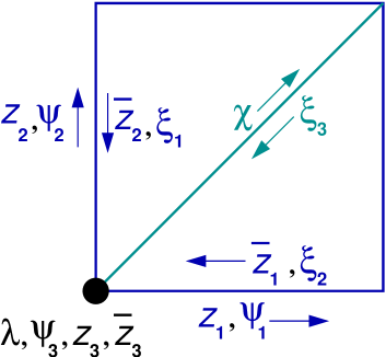
Figure 3: The lattice for SYM in $d=2$ with ${\cal Q}=8$ supercharges. the $z_{i}$ are complex bosons, while the other fields are one-component fermions.

The lattice action is given by

$$S=\frac{1}{g^{2}} \sum_{{\bf n}}{\rm Tr}\,\biggl{[}2\left|\epsilon_{ij}z_{i,{\bf n}}z_{j,{\bf n}+\mathbf{\hat{e}}_{i}}\right|^{2}$$ (16)

$$+2\left|z_{i,{\bf n}}z_{3,{\bf n}+\mathbf{\hat{e}}_{i}}-z_{3,{\bf n}}z_{i,{\bf n}}\right|^{2}$$

$${\textstyle{\frac{1}{2}}}\left(\kern 0.6pt\overline{\kern-0.6ptz\kern-0.6pt}\kern 0.6pt_{i,{\bf n}-\mathbf{\hat{e}}_{i}}z_{i,{\bf n}-\mathbf{\hat{e}}_{i}}-z_{i,{\bf n}}\kern 0.6pt\overline{\kern-0.6ptz\kern-0.6pt}\kern 0.6pt_{i,{\bf n}}+[\kern 0.6pt\overline{\kern-0.6ptz\kern-0.6pt}\kern 0.6pt_{3,{\bf n}},\,z_{3,{\bf n}}]\right)^{2}$$

$$+\sqrt{2}\Bigl{(}\Delta_{\bf n}(\lambda,\kern 0.6pt\overline{\kern-0.6ptz\kern-0.6pt}\kern 0.6pt_{a},\psi_{a})-\Delta_{\bf n}(\chi,\kern 0.6pt\overline{\kern-0.6ptz\kern-0.6pt}\kern 0.6pt_{a},\xi_{a})$$

$$\qquad\quad+\epsilon_{abc}\Delta_{\bf n}(\psi_{a},z_{b},\xi_{c})\Bigr{)}$$

where the $\Delta$ functions have the same structure seen in Eq. (3).

As before, analysis of the continuum limit is facilitated by making the supersymmetry explicit. A superfield notation is again possible by introducing two independent Grassmann variables $\theta$ and $\kern 0.6pt\overline{\kern-0.6pt\theta\kern-0.6pt}\kern 0.6pt$. There are seven bosonic superfields $Z_{i}$, $\kern 0.6pt\overline{\kern-0.6ptZ\kern-0.6pt}\kern 0.6pt_{i}$, and $S$, and three Grassmann superfields $\Upsilon$, $\kern 0.6pt\overline{\kern-0.6pt\Upsilon\kern-0.6pt}\kern 0.6pt$ and $\Xi$. Here are some examples of how several of the superfields are related to component fields:

$${\mathbf{Z}_{i,{\bf n}}} =z_{i,{\bf n}}+\sqrt{2}\,\theta\psi_{i,{\bf n}}$$ (17)

$$\quad-\sqrt{2}\,\theta{\kern 0.6pt\overline{\kern-0.6pt\theta\kern-0.6pt}\kern 0.6pt}(\kern 0.6pt\overline{\kern-0.6ptz\kern-0.6pt}\kern 0.6pt_{3,{\bf n}}z_{i,{\bf n}}-z_{i,{\bf n}}\kern 0.6pt\overline{\kern-0.6ptz\kern-0.6pt}\kern 0.6pt_{3,{\bf n}+\mathbf{\hat{e}}_{i}})\$$

$${\boldsymbol{\Xi}_{\bf n}} =\xi_{3,{\bf n}}+\sqrt{2}\,\theta\Bigl{(}G_{\bf n}-\sqrt{2}\,\epsilon_{ij}\,\kern 0.6pt\overline{\kern-0.6ptz\kern-0.6pt}\kern 0.6pt_{i,{\bf n}+\mathbf{\hat{e}}_{j}}\kern 0.6pt\overline{\kern-0.6ptz\kern-0.6pt}\kern 0.6pt_{j,{\bf n}}\Bigr{)}$$

$$\quad-\sqrt{2}\,\theta{\kern 0.6pt\overline{\kern-0.6pt\theta\kern-0.6pt}\kern 0.6pt}(\kern 0.6pt\overline{\kern-0.6ptz\kern-0.6pt}\kern 0.6pt_{3,{\bf n}+\mathbf{\hat{e}}_{1}+\mathbf{\hat{e}}_{2}}\xi_{3,{\bf n}}-\kern 0.6pt\overline{\kern-0.6ptz\kern-0.6pt}\kern 0.6pt_{3,{\bf n}}\xi_{3,{\bf n}})\ ,$$

$${\boldsymbol{\Upsilon}}_{\bf n} =\lambda_{\bf n}-\theta\Bigl{(}\kern 0.6pt\overline{\kern-0.6ptz\kern-0.6pt}\kern 0.6pt_{i,{\bf n}-\mathbf{\hat{e}}_{i}}z_{i,{\bf n}-\mathbf{\hat{e}}_{i}}-z_{i,{\bf n}}\kern 0.6pt\overline{\kern-0.6ptz\kern-0.6pt}\kern 0.6pt_{i,{\bf n}}$$

$$\quad+[\kern 0.6pt\overline{\kern-0.6ptz\kern-0.6pt}\kern 0.6pt_{3,{\bf n}},z_{3,{\bf n}}]+id_{\bf n}\Bigr{)}-\sqrt{2}\theta\kern 0.6pt\overline{\kern-0.6pt\theta\kern-0.6pt}\kern 0.6pt[\kern 0.6pt\overline{\kern-0.6ptz\kern-0.6pt}\kern 0.6pt_{3,{\bf n}},\lambda_{\bf n}]\ .$$

The action of the two supercharges on the superfields is given by

$$Q=\frac{\partial\ }{\partial\theta}+\sqrt{2}\,\kern 0.6pt\overline{\kern-0.6pt\theta\kern-0.6pt}\kern 0.6pt[\kern 0.6pt\overline{\kern-0.6ptz\kern-0.6pt}\kern 0.6pt_{3},\,\cdot\ ]\ ,\quad\kern 0.6pt\overline{\kern-0.6ptQ\kern-0.6pt}\kern 0.6pt=\frac{\partial\ }{\partial\kern 0.6pt\overline{\kern-0.6pt\theta\kern-0.6pt}\kern 0.6pt}+\sqrt{2}\,\theta[\kern 0.6pt\overline{\kern-0.6ptz\kern-0.6pt}\kern 0.6pt_{3},\,\cdot\ ]\ ,$$ (18)

with the nontrivial anti-commutator $\{Q,\kern 0.6pt\overline{\kern-0.6ptQ\kern-0.6pt}\kern 0.6pt\}=2\sqrt{2}[\kern 0.6pt\overline{\kern-0.6ptz\kern-0.6pt}\kern 0.6pt_{3},\,\cdot\ ]$. To obtain an off-shell realization of the super-algebra required introducing two auxiliary fields, $d$ and $G$. Note that again the supermultiplets are not entirely local, which is what leads to supersymmetry charges being related to translations in the continuum.

As in the ${\cal Q}=4$ example, the continuum limit of the $d=2$, ${\cal Q}=8$ lattice is defined as an expansion about the point in moduli space

$$\langle z_{1}\rangle=\langle z_{2}\rangle=\frac{1}{\sqrt{2}\,a}\ ,$$ (19)

in the limit

$$a\to 0,\quad g\to\infty\ ,\quad ga=g_{2}\ {\text{fixed}}.$$ (20)

Again one finds that at the classical level, the lattice theory Eq. (16) yields the target theory Eq. (15) with the complex $z_{3}$ and the real parts of $z_{1,2}$ forming the four real scalars $s_{\mu}$ of the target theory, while the fermions arrange themselves as

$$\kern 0.6pt\overline{\kern-0.6pt\Psi\kern-0.6pt}\kern 0.6pt_{1} =\begin{pmatrix}-\chi&\psi_{3}\end{pmatrix}\ , \quad\kern 0.6pt\overline{\kern-0.6pt\Psi\kern-0.6pt}\kern 0.6pt_{2} =\begin{pmatrix}\psi_{1}&\psi_{2}\end{pmatrix}\ ,$$ (21)

$$\Psi_{1} =\begin{pmatrix}\xi_{1}\\ \xi_{2}\end{pmatrix}\ , \quad\Psi_{2} =\begin{pmatrix}\ \lambda\\ -\xi_{3}\end{pmatrix}\ ,\quad$$ (22)

Furthermore, an analysis of the radiative corrections again reveals that no fine-tuning is required to obtain the ${\cal Q}=8$ target theory of Eq. (15) continuum limit. I refer you to Ref. [17] for details.

5 Constructing the supersymmetric lattices

I purposely did not begin this talk by explaining how to construct the supersymmetric lattices I have presented. The technique is described in detail in Refs. [14, 15, 16, 17], and explaining it in a dark room tends to encourage people to go to sleep. But at this point I have nothing to lose, so here is a brief overview of the recipe.

For a target SYM theory in $d$ dimensions with a $U(k)$ gauge group and ${\cal Q}$ real supercharges:

• Begin with a SYM theory in the continuum with ${\cal Q}$ supercharges, but with the much bigger gauge group $U({k}{N}^{{d}})$;

• Reduce the theory to zero dimensions, yielding a matrix model, with ${{\cal Q}}$ supersymmetries, and a $U({k}{N}^{{d}})\times G_{R}$ global symmetry

  • For ${{\cal Q}}=4$, $G_{R}=SO(4)\times U(1)$;

  • For ${{\cal Q}}=8$, $G_{R}=SO(6)\times SU(2)$;

  • For ${{\cal Q}}=16$, $G_{R}=SO(10)$.

  $G_{R}$ is an “$R$-symmetry” which does not commute with the supercharges. These $G_{R}$ groups are uniquely determined by the number of supercharges ${\cal Q}$.

• Identify a particular $(Z_{{N}})^{{d}}$ subgroup of the $U({k}{N}^{{d}})\times G_{R}$ symmetry. Remove from the matrix model any variables which transform non-trivially under this discrete symmetry (a process called “orbifolding”).

I will illustrate how this sequence of steps was followed to produce the $d=2$, ${\cal Q}=4$ lattice discussed in § 3.

Step 1: We desire a matrix model with ${\cal Q}=4$ supercharges and a $U(kN^{2})$ gauge symmetry. This is easily constructed by starting with the familiar ${\cal N}=1$ SYM theory in four dimensions, and then erasing the spacetime dependence of all the fields. We are left with the matrix model

$$S=\frac{1}{g^{2}}{\rm Tr}\,\left(\frac{1}{4}v_{mn}v_{mn}+\kern 0.6pt\overline{\kern-0.6pt\psi\kern-0.6pt}\kern 0.6pt\kern 0.6pt\overline{\kern-0.6pt\sigma\kern-0.6pt}\kern 0.6pt_{m}[v_{m},\psi]\right)$$ (23)

where $m=0,\ldots,4$, $\kern 0.6pt\overline{\kern-0.6pt\sigma\kern-0.6pt}\kern 0.6pt_{m}=\{1,i\vec{\sigma}\}$ (where $\vec{\sigma}$ are the three Pauli matrices), and $v_{mn}=i[v_{m},v_{n}]$. The fields $\psi$, $\kern 0.6pt\overline{\kern-0.6pt\psi\kern-0.6pt}\kern 0.6pt$ and $v_{m}$ are all $kN^{2}$ dimensional-matrices. The symmetries of the action $S$ are: (i) $U(kN^{2})$, under which $v_{m}\to Uv_{m}U^{\dagger}$, and similarly for $\psi$ and $\kern 0.6pt\overline{\kern-0.6pt\psi\kern-0.6pt}\kern 0.6pt$; (ii) an $R$-symmetry $G_{R}=SO(4)\times U(1)$ under which $v_{m}$ transforms as a neutral 4-vector, while $\psi$ and $\kern 0.6pt\overline{\kern-0.6pt\psi\kern-0.6pt}\kern 0.6pt$ transform as charged spinors; and (iii) ${\cal Q}=4$ supersymmetry, consisting of the following transformations

$$\delta\psi =-iv_{mn}\sigma_{mn}\kappa\ ,$$ (24)

$$\delta\kern 0.6pt\overline{\kern-0.6pt\psi\kern-0.6pt}\kern 0.6pt =iv_{mn}\kern 0.6pt\overline{\kern-0.6pt\kappa\kern-0.6pt}\kern 0.6pt\kern 0.6pt\overline{\kern-0.6pt\sigma\kern-0.6pt}\kern 0.6pt_{mn}\ ,$$

$$\delta v_{m} =-i\left(\kern 0.6pt\overline{\kern-0.6pt\psi\kern-0.6pt}\kern 0.6pt\kern 0.6pt\overline{\kern-0.6pt\sigma\kern-0.6pt}\kern 0.6pt_{m}\kappa-\kern 0.6pt\overline{\kern-0.6pt\kappa\kern-0.6pt}\kern 0.6pt\sigma_{m}\psi\right)\ ,$$

with $\kern 0.6pt\overline{\kern-0.6pt\sigma\kern-0.6pt}\kern 0.6pt_{m}=\sigma_{m}^{\dagger}$ and $\sigma_{mn}=\frac{1}{4}(\sigma_{m}\kern 0.6pt\overline{\kern-0.6pt\sigma\kern-0.6pt}\kern 0.6pt_{n}-\sigma_{n}\kern 0.6pt\overline{\kern-0.6pt\sigma\kern-0.6pt}\kern 0.6pt_{m})$; $\kappa$ and $\kern 0.6pt\overline{\kern-0.6pt\kappa\kern-0.6pt}\kern 0.6pt$ are independent two-component Grassmann spinor parameters.

Step 2: Next we project out a $Z_{N}\times Z_{N}$ symmetry, which means that we identify a particular $Z_{N}\times Z_{N}$ subgroup of the global $U(kN^{2})\times SO(4)\times U(1)$ symmetry of our matrix model, and then set to zero all fields except those which are neutral under this discrete symmetry. The result is to render the $kN^{2}$-dimensional matrix variables sparse, inhabited by only $N^{2}$ $k$-dimensional blocks. These nonzero blocks will be identified with $k$-dimensional matrix variables inhabiting the sites or links of the $N^{2}$ cells of the two dimensional lattice, as shown in Fig. 1.

The details of how this projection works are given in Ref. [16] and won’t be repeated here, but the procedure may be illustrated by a toy example of two $3k$-dimensional matrix fields $\Phi_{0}$ and $\Phi_{1}$. Assume that we have an action $S$ depending on $\Phi_{0}$ and $\Phi_{1}$ which is invariant under a $U(3k)\times U(1)$ symmetry, where $\Phi_{0}$ and $\Phi_{1}$ are both $U(3k)$ adjoints with $U(1)$ charges $0$ and $1$ respectively (the $U(1)$ plays the role of $G_{R}$). We can define a $Z_{3}\subset U(3k)\times U(1)$ subgroup whose action on the two fields is

$$\Phi_{q}\to e^{i(2\pi q)/3}U\Phi_{q}U^{\dagger},\quad U\equiv\begin{pmatrix}1&&&\cr&\omega&&\cr&&\omega^{2}&\end{pmatrix}\ ,$$ (25)

with $\omega=e^{2\pi i/3}\times\boldsymbol{1_{k}}$. Setting to zero all components of $\Phi_{0,1}$ except those which are invariant under this $Z_{3}$ symmetry results in $\Phi_{0}$ consisting of three nonzero $k$-dimensional blocks along the diagonal, and $\Phi_{1}$ consisting of three nonzero $k$-dimensional blocks in the $\{12\}$, $\{23\}$ and $\{31\}$ positions. We can interpret these remaining variables as degrees of freedom on a three-site, one-dimensional lattice with periodic boundary conditions—the three blocks in $\Phi_{0}$ become site variables, while those in $\Phi_{1}$ become link variables. Substituting the projected $\Phi$ matrices back into the original action results in a lattice action that respects a $U(k)^{3}$ subgroup of the original $U(3k)$ symmetry, with a $U(k)$ factor associated with each of the three sites. The $Z_{N}\times Z_{N}$ projection of the matrix model Eq. (23) works similarly, except that we get an $N$-site dimension for each of the two $Z_{N}$ factors, resulting in a two-dimensional, $N^{2}$-site lattice.

The supersymmetric lattices we construct suffer from two general limitations: Firstly, the group $G_{R}$ needs to be able to contain a $Z_{N}^{d}$ subgroup, which means that it has to be at least of rank $d$. Secondly, projecting out a $Z_{N}$ always breaks at least half of the supersymmetries. This means that lattices for higher dimensional theories are in general less supersymmetric, and therefore less well protected from radiative corrections. For example, if we tried to construct a lattice action for $d=3$, ${\cal Q}=4$ SYM theory, we would find that the lattice would not respect any exact supersymmetries, and so would presumably require fine-tuning. It is impossible to construct any lattice for ${\cal Q}=4$ SYM in $d=4$ following our method, since for ${\cal Q}=4$, $G_{R}=SO(4)\times U(1)$ which is only rank three.

6 The bestiary of supersymmetric lattices

I now give a quick survey of the various supersymmetric lattices we have succeeded in constructing. The ${\cal Q}=4$ and ${\cal Q}=8$ lattices are discussed in Refs. [16], [17] respectively; a paper on ${\cal Q}=16$ target theories is in preparation, and our work on Euclidean lattices in $d=1$ is unpublished.

One-dimensional lattices. We can construct one dimensional lattices for supersymmetric quantum mechanics with ${\cal Q}=2,4,8$, or $16$ supercharges, with ${\cal Q}/2$ of those supercharges realized exactly on the lattice. No fine-tuning is required for any of these theories. These may prove to be the most reasonable starting point for a numerical investigation of supersymmetric lattices, as one may be able to use conventional Hamiltonian techniques with which to compare the answers obtained from a latticized path integral. Furthermore, the ${\cal Q}=16$ case is interesting in its own right, as it is believed that the large $N_{c}$ limit of such a theory is in fact $M$-theory [24]. Understanding this theory could conceivably answer questions about quantum gravity.

Two-dimensional lattices. Beside the ${\cal Q}=4$ and ${\cal Q}=8$ examples I have discussed, we can also construct the $d=2$, ${\cal Q}=16$ lattice which has the triangular structure shown in Fig. 4. This lattice respects four exact supersymmetries, and requires no fine-tuning.

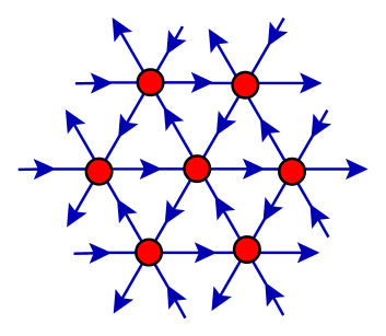
Figure 4: The lattice for SYM in $d=2$ with ${\cal Q}=16$ supercharges.

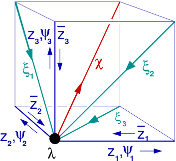
Figure 5: The lattice for SYM in $d=3$ with ${\cal Q}=8$ supercharges.

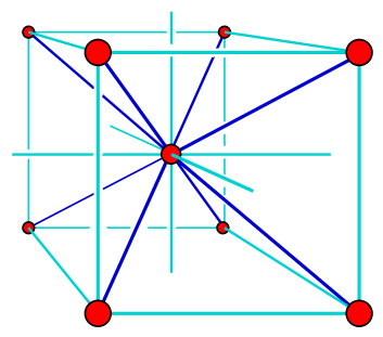
Figure 6: The bcc lattice for SYM in $d=3$ with ${\cal Q}=16$ supercharges. Link orientation and particle content are not shown.

Three-dimensional lattices. We can construct $d=3$ lattices for ${\cal Q}=8$ and ${\cal Q}=16$ which respect one and two exact supercharges respectively. The lattices take the form shown in Fig. 5 and Fig. 6 respectively. We find that two fine-tunings are indicated in the ${\cal Q}=8$ case, but none for ${\cal Q}=16$. These theories both have interesting features. The ${\cal Q}=8$ SYM theory possesses something called “mirror symmetry”, which has been analyzed in Ref. [25], while the ${\cal Q}=16$ theory is expected to have a nontrivial infrared fixed point [26]. required.

A four-dimensional lattice. The only $d=4$ lattice we can construct has as its target theory ${\cal N}=4$ SYM. The target theory is expected to be finite, and its large-$N_{c}$ limit is expected to have a dual string theory description. The lattice we construct is of the $A_{4}^{*}$ type [27]; it respects a single exact supersymmetry. In this case it appears that the supersymmetry of the lattice is not sufficiently powerful to eliminate the need for fine-tuning, but we have not yet explored how many fine-tunings are

Spatial lattices. Up to now I have only discussed Euclidean lattices, but it is also possible to construct spatial lattices in continuous Minkowski time for a Hamiltonian approach [14]. The advantage of these lattices is that, being lower by one dimension from the corresponding Euclidean lattices, they possess twice as many exact supersymmetries. This suffices, for example, to eliminate the need for fine-tuning in the $d=3$, ${\cal Q}=8$ case. Fine-tuning may be required for the ${\cal Q}=16$ lattice in $d=3+1$ dimensions, but that is not certain [14].

7 Future directions

I hope I have given you a sense of the unusual and beautiful properties of these supersymmetric lattices, and how they circumvent the apparent obstacles discussed in §2 — such as the need for chiral symmetries in the continuum — in devious and novel ways. I hope that further study will enlarge the class of supersymmetric theories that can be constructed on the lattice, perhaps making contact with the ideas presented at this conference by Simon Catterall. I am also optimistic that these lattices may prove useful for analytical studies of supersymmetry, perhaps allowing one to construct explicit Nicolai maps [28] in a regulated theory, or leading to a better understanding of duality in SYM theories. Eventually I hope that such lattices could provide a window onto quantum gravity through the connection discovered between string theories and SYM in the large-$N_{c}$ limit.

The greatest obstacle now to numerical study of these theories is the issue of simulating dynamical fermions. Not only is there the challenge of exactly massless fermions, but apparently there is a sign problem as well [29, 30]. It can be shown analytically that the sign problem must disappear in the continuum limit for the ${\cal Q}=4$ lattices, but it is unknown what happens in the cases with more supersymmetry. In any case, it would seem that analysis of one-dimensional lattices for a path integral formulation of supersymmetric quantum mechanics would be the technically most feasible place to start any investigation.

References

- [1] N. Seiberg and E. Witten, Nucl. Phys. B431 (1994) 484, hep-th/9408099,
- [2] J. Terning, (2003), hep-th/0306119,
- [3] I.R. Klebanov, (2000), hep-th/0009139,
- [4] S. Catterall and S. Karamov, Phys. Rev. D65 (2002) 094501, hep-lat/0108024,
- [5] S. Catterall and S. Karamov, Phys. Rev. D68 (2003) 014503, hep-lat/0305002,
- [6] M. Beccaria, M. Campostrini and A. Feo, Nucl. Phys. Proc. Suppl. 106 (2002) 944, hep-lat/0110056,
- [7] K. Fujikawa, (2002), hep-th/0205095,
- [8] I. Montvay, (2001), hep-lat/0112007,
- [9] A. Feo, (2002), hep-lat/0210015,
- [10] A. Feo, (2003), hep-lat/0305020,
- [11] S. Catterall, JHEP 05 (2003) 038, hep-lat/0301028,
- [12] J. Nishimura, S.J. Rey and F. Sugino, JHEP 02 (2003) 032, hep-lat/0301025,
- [13] K. Itoh et al., JHEP 02 (2003) 033, hep-lat/0210049,
- [14] D.B. Kaplan, E. Katz and M. Unsal, JHEP 05 (2003) 037, hep-lat/0206019,
- [15] D.B. Kaplan, (2002), hep-lat/0208046,
- [16] A.G. Cohen et al., JHEP 08 (2003) 024, hep-lat/0302017,
- [17] A.G. Cohen et al., (2003), hep-lat/0307012,
- [18] D.B. Kaplan, Phys. Lett. B136 (1984) 162,
- [19] H. Neuberger, Phys. Rev. D57 (1998) 5417, hep-lat/9710089,
- [20] D.B. Kaplan and M. Schmaltz, Chin. J. Phys. 38 (2000) 543, hep-lat/0002030,
- [21] J. Nishimura, Phys. Lett. B406 (1997) 215, hep-lat/9701013,
- [22] G.T. Fleming, J.B. Kogut and P.M. Vranas, Phys. Rev. D64 (2001) 034510, hep-lat/0008009,
- [23] T. Banks and P. Windey, Nucl. Phys. B198 (1982) 226,
- [24] T. Banks et al., Phys. Rev. D55 (1997) 5112, hep-th/9610043,
- [25] A. Kapustin and M.J. Strassler, JHEP 04 (1999) 021, hep-th/9902033,
- [26] N. Seiberg, Nucl. Phys. Proc. Suppl. 67 (1998) 158, hep-th/9705117,
- [27] J.H. Conway and N.J.A. Sloane, New York, USA: Springer-Verlag (1991) 703 P. (Grundlehren der mathematischen Wissenschaften 290).
- [28] H. Nicolai, Phys. Lett. B89 (1980) 341,
- [29] J. Giedt, Nucl. Phys. B668 (2003) 138, hep-lat/0304006,
- [30] J. Giedt, (2003), hep-lat/0307024,