HU-EP-03/61 DESY 03-137 SFB/CPP-03-38 September 2003
Simulating the Schrödinger functional with two pseudo-fermions: algorithmic study and the running mass

Abstract

We present an algorithmic study for the simulation of two massless flavors of O(a) improved Wilson quarks with Schrödinger functional boundary conditions. The algorithm used is Hybrid Monte Carlo with two pseudo-fermion fields as proposed by M. Hasenbusch. A gain in CPU cost of a factor two is reached when compared to one pseudo-fermion field due to the larger possible step-size. This study is integrated in the ALPHA project for the computation of the running of the renormalized quark mass. We include an update on these physics results.

1 HMC with two pseudo-fermion fields

We study [1] a variant of the Hybrid Monte Carlo (HMC) algorithm that uses two pseudo-fermion fields per degenerate flavor doublet, as proposed by M. Hasenbusch [2, 3] and recently tested in [4]. The Wilson-Dirac operator with Schrödinger functional (SF) boundary conditions $D_{\rm w}+m_{0}$ is considered together with O($a$) improvement $\delta D$ respectively $T$ (clover term) and even-odd preconditioning

$$a(D_{\rm w}+\delta D+m_{0})=\frac{1}{2\kappa}M\,,$$ (1)

$$M=\left(\begin{array}[]{cc}1+T_{ee}&M_{eo}\\ M_{oe}&1+T_{oo}\end{array}\right)\,.$$ (4)

For one mass-degenerate flavor doublet of quarks the partition function reads

$$Z = \int_{U}\exp(-S_{\rm g}(U))\det(1+T_{ee})^{2}\det{\hat{Q}}^{2}\,,$$ (5)

$$\hat{Q} = \tilde{c}_{0}\gamma_{5}\{1+T_{oo}-M_{oe}(1+T_{ee})^{-1}M_{eo}\}\,,$$ (6)

with $\tilde{c}_{0}=(1+64\kappa^{2})^{-1}$ and $S_{\rm g}(U)$ is the Wilson plaquette action. To simulate eq. (5) we use the Hybrid Monte Carlo algorithm. The determinant $\det{\hat{Q}}^{2}$ is represented in terms of pseudo-fermion fields $\phi$. If $\hat{Q}$ is factorized in $n_{\rm pf}$ factors then one pseudo-fermion field for each factor is introduced. The aim of the factorization is to make the fermionic contribution to the forces associated with each factor as small as possible. We take $n_{\rm pf}=2$ and the factorization

$$\hat{Q}=(\tilde{Q})(\tilde{Q}^{-1}\hat{Q})\,,\quad\tilde{Q}=\hat{Q}-i\rho\,,$$ (7)

which leads to the pseudo-fermion actions $i=1,2$

$$S_{{\rm F}_{i}}=\phi_{i}^{\dagger}\left[\sigma_{i}^{2}+(\hat{Q}^{2}+\rho_{i}^{2})^{-1}\right]\phi_{i}\,,$$ (8)

$$\sigma_{1}=0\,,\;\rho_{1}=\rho\,,\quad\sigma_{2}=\frac{1}{\rho}\,,\;\rho_{2}=0\,.$$ (9)

The real parameter $\rho$ is chosen to minimize the sum of the condition numbers of the two operators appearing in eq. (8),

$$\rho = \left[\lambda_{\min}(\hat{Q}^{2})\lambda_{\max}(\hat{Q}^{2})\right]^{1/4}\,,$$ (10)

in terms of the smallest and largest eigenvalue of $\hat{Q}^{2}$. The operators in eq. (8) have then both condition number equal to the square root of the condition number of $\hat{Q}^{2}$.

This algorithmic study is part of the ALPHA large scale simulations for the computation of the running of the renormalized quark mass [5]. For the temporal and spatial lattice size, the background gauge field and the parameter controlling the spatial boundary conditions of the fermion fields we take respectively

$$T=L\,,\quad C=C^{\prime}=0\,,\quad\theta=0.5\,.$$ (11)

The theory is simulated along the critical line where the PCAC mass vanishes. These simulations are possible in the SF due to the infrared cut-off proportional to $1/T^{2}$ in the spectrum of the Dirac operator squared. In our simulations the renormalized coupling $u=\bar{g}^{2}(L)$ [6] takes values in the range $u=1.0\ldots 5.7$. In the SF $u$ is presumably a monotonically growing function of $L$ and our simulations correspond approximately to the range $L=10^{-2}\ldots 1\,{\rm fm}$.

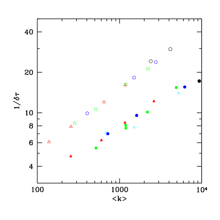
Figure 1: Step-sizes $\delta\tau$ for 80% acceptance. Open symbols are for $n_{\rm pf}=1$, filled symbols and crosses for $n_{\rm pf}=2$.

2 PERFORMANCE

In the integration of the molecular dynamics equations of motion we adjust the step-size $\delta\tau$ to yield an acceptance of 80% for trajectories of length one. Fig. 1 shows the inverse step-size, i.e. the number of steps, as a function of the average condition number of $\hat{Q}^{2}$

$$\langle k\rangle=\Big{\langle}\frac{\lambda_{\max}(\hat{Q}^{2})}{\lambda_{\min}(\hat{Q}^{2})}\Big{\rangle}\,.$$ (12)

Data are shown for different lattice sizes $L/a$ and renormalized couplings $u=1.0,1.1$ (triangles), $u=2.5$ (squares), $u=3.3$ (pentagons), $u=5.7$ (circles) together with simulations at $\beta=5.2,\;\kappa=0.1355$ (crosses). The filled symbols and crosses are obtained with $n_{\rm pf}=2$ and the open symbols with $n_{\rm pf}=1$ (standard HMC). With $n_{\rm pf}=2$ we can choose step-sizes which are a factor two larger than with $n_{\rm pf}=1$.

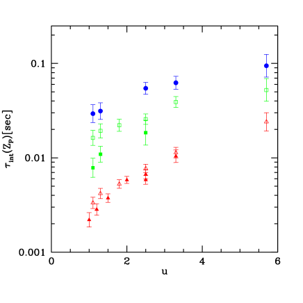
Figure 2: Integrated autocorrelation time of $Z_{\rm P}$. Data are for lattices $L/a=12$ (triangles), $L/a=16$ (squares) and $L/a=24$ (circles), open symbols for $n_{\rm pf}=1$ and filled symbols for $n_{\rm pf}=2$.

In Fig. 2 we plot the integrated autocorrelation time $\tau_{\rm int}(Z_{\rm P})$ [7] of the pseudoscalar density $Z_{\rm P}$ as a function of $u$. $Z_{\rm P}$ is the quantity we need in order to compute the running of the renormalized mass. The units are CPU seconds per lattice point for the simulation of one lattice on one APEmille crate, which consists of 128 nodes and has a peak performance of 68 GFlops. Data are for lattices $L/a=12$ (triangles), $L/a=16$ (squares) and $L/a=24$ (circles), open symbols for $n_{\rm pf}=1$ and filled symbols for $n_{\rm pf}=2$. A systematic difference between $n_{\rm pf}=1$ and $n_{\rm pf}=2$ is seen for the $L/a=16$ lattices, the smallest couplings show a reduction in CPU cost by about a factor two for $n_{\rm pf}=2$. This CPU gain is due to the larger possible step-size. A comparison at $L/a=24$ would demand too much CPU time, precisely because of this it was essential to our project to speed up the standard HMC.

3 THE RUNNING MASS

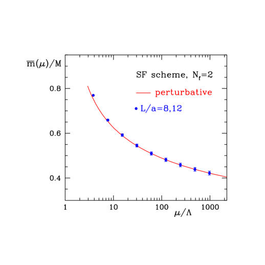
Figure 3: The running of the renormalized quark mass.

The running of the renormalized quark mass $\overline{m}(\mu)$ with the renormalization scale $\mu=1/L$ is extracted from the step scaling function $\sigma(u)$ of the coupling and the step scaling function $\sigma_{\rm P}(u)$ of the pseudoscalar density,

$$\sigma(u) = \bar{g}^{2}(2L)\,,\quad u=\bar{g}^{2}(L)\,,$$ (13)

$$\sigma_{\rm P}(u) = \left.\lim_{a/L\to 0}\,\frac{Z_{\rm P}(g_{0},2L/a)}{Z_{\rm P}(g_{0},L/a)}\right|_{u=\bar{g}^{2}(L)}$$ (14)

$$= \frac{\overline{m}(1/L)}{\overline{m}(1/2L)}\,.$$ (15)

We solve the joint recursion: $k=0,1,2,\ldots$

$$\left\{\begin{array}[]{l}u_{0}=\bar{g}^{2}(L_{\rm max})=4.6800\\ \sigma(u_{k+1})=u_{k}\end{array}\right.\,,$$ (18)

$$\Rightarrow u_{k}=\bar{g}^{2}(L_{k})\,,\quad L_{k}=2^{-k}L_{\rm max}\,,$$ (19)

$$w_{0}=1\,,\quad w_{k}=\left[\prod_{i=1}^{k}\sigma_{\rm P}(u_{i})\right]^{-1}\,,$$ (20)

$$\Rightarrow w_{k}=\frac{\overline{m}(1/L_{\rm max})}{\overline{m}(1/L_{k})}\,,$$ (21)

which gives the running of $\overline{m}(\mu)$ starting at the scale $1/L_{\rm max}$ defined by $\bar{g}^{2}(L_{\rm max})=4.6800$.

For the step scaling function $\sigma_{\rm P}(u)$ we take the average $\overline{\Sigma}_{\rm P}^{(8,12)}(u)$ of its values $\Sigma_{\rm P}(u,a/L)$, which we computed on $L/a=8,12$ (and $2L/a$) lattices for 6 couplings in the range $u=0.98\dots 3.3$. Then we interpolate by the Ansatz

$$\overline{\Sigma}_{\rm P}^{(8,12)}(u) = 1-\ln(2)d_{0}u+p_{2}u^{2}+p_{3}u^{3}$$ (22)

with $d_{0}$ perturbative, fitted parameters $p_{2}$ and $p_{3}$ and use this fit formula in the recursion eq. (20). At high energies contact with the perturbative regime is made from which the RGI parameters $\Lambda$ and $M$ can be extracted [1]

$$\ln(\Lambda L_{\rm max})=-1.34(7)$$ (23)

$$\frac{M}{\overline{m}(1/L_{\rm max})}=1.30(3)\,.$$ (24)

Fig. 3 is then obtained from the coefficients eq. (19) and eq. (21). The errors of the points come from the statistical errors in the coefficients $w_{k}$, the scale ambiguities in the quantities $\Lambda L_{\rm max}$ and $M/\overline{m}(1/L_{\rm max})$ are not shown.

The outlook of this work is the determination of $L_{\rm max}$ using available data from JLQCD [8] and UKQCD [9]. A hadronic scheme has to be set up to determine combinations of $M_{u}$, $M_{d}$ and $M_{s}$.

Acknowledgement. We thank NIC/DESY Zeuthen for allocating computer time on the APEmille machine and the APE group for their support. This work was supported by the European Community’s Human Potential Programme under contract HPRN-CT-2000-00145 and by the Deutsche Forschungsgemeinschaft in the SFB/TR 09.

References

- [1] M. Della Morte et al. (ALPHA collaboration), (2003), hep-lat/0307008, to appear in Comput. Phys. Commun..
- [2] M. Hasenbusch, Phys. Lett. B519, (2001) 177; M. Hasenbusch and K. Jansen, Nucl. Phys. B659, (2003) 299.
- [3] M. Hasenbusch, “Full QCD Algorithms toward the Chiral Limit”, these proceedings.
- [4] A. Ali Khan et al. (QCDSF collaboration), Phys. Lett. B564, (2003) 235; H. Stüben (QCDSF collaboration), these proceedings.
- [5] F. Knechtli et al. (ALPHA collaboration), Nucl. Phys. B Proc. Suppl. 119, (2003) 320.
- [6] A. Bode et al. (ALPHA collaboration), Phys. Lett. B515, (2001) 49.
- [7] U. Wolff, (2003), hep-lat/0306017.
- [8] S. Aoki et al. (JLQCD collaboration), (2002), hep-lat/0212039.
- [9] C.R. Allton et al. (UKQCD collaboration), Phys. Rev. D65, (2002) 054502.