Moments of nucleon spin-dependent generalized parton distributions

Abstract

We present a lattice measurement of the first two moments of the spin-dependent GPD $\tilde{H}(x,\xi,t)$. From these we obtain the axial coupling constant and the second moment of the spin-dependent forward parton distribution. The measurements are done in full QCD using Wilson fermions. In addition, we also present results from a first exploratory study of full QCD using Asqtad sea and domain-wall valence fermions.

1 INTRODUCTION

Generalized parton distributions (GPDs) [1] (see also [2] for a recent review) provide a means of parametrizing hadronic contributions to both exclusive and inclusive processes. They reduce in certain limits to form factors and to (forward) parton distributions. For a review on the nucleon axial structure see [3] and for spin-dependent parton distributions consult [4].

GPDs depend on three independent kinematic variables and are therefore far more difficult to extract from experiments than forward parton distributions. Lattice simulations provide a general, model-independent way to compute their moments directly. First results for spin-independent GPDs have been presented in [5]. These papers, however, concentrate on rather large quark masses. It is imperative to extend these studies down into the chiral regime.

In this talk, we will present a first study of spin-dependent GPDs, both with Wilson fermions at large quark masses and with staggered sea and domain-wall valence fermions at intermediate quark masses.

2 PARAMETRIZATION

Spin-dependent GPDs are specified by $\tilde{E}^{\mbox{\tiny f}}(x,\xi,t)$ and $\tilde{H}^{\mbox{\tiny f}}(x,\xi,t)$, defined via

$$\!\!\!\!\bar{p}^{+}\int\frac{dz^{-}}{2\pi}e^{\mbox{\tiny i}\bar{p}^{+}z^{-}}\langle p^{\prime}|\bar{\psi}^{\mbox{\tiny f}}(-z^{-}/2)\gamma_{5}\gamma^{+}\psi^{\mbox{\tiny f}}(z^{-}/2)|p\rangle$$

$$\!\!\!=\tilde{H}^{\mbox{\tiny f}}(x,\xi,t)\langle\!\langle\gamma_{5}\gamma^{+}\rangle\!\rangle-\tilde{E}^{\mbox{\tiny f}}(x,\xi,t)\frac{\Delta^{+}}{2m}\langle\!\langle\gamma_{5}\rangle\!\rangle\,.$$ (1)

The upper index f denotes the quark flavor, $x$ is the average longitudinal momentum fraction of the struck quark, and $\xi$ the longitudinal momentum transfer. The total invariant momentum transfer squared is given by $t\equiv\Delta^{2}$, with the four-momentum transfer $\Delta=p^{\prime}-p$. The average hadron momentum is denoted by $\bar{p}=(p^{\prime}+p)/2$. We also use the short-hand notation $\langle\!\langle\Gamma\rangle\!\rangle=\bar{u}(p^{\prime})\Gamma u(p)$.

By taking moments with respect to $x$, we end up with a tower of local matrix elements of the form

$$\langle p^{\prime}|\bar{\psi}^{\mbox{\tiny f}}\gamma^{\{\mu_{1}}\gamma_{5}\mbox{i}D^{\mu_{2}}\cdots\mbox{i}D^{\mu_{n}\}}\psi^{\mbox{\tiny f}}|p\rangle\,.$$ (2)

SESAM $\Omega=16^{3}\times 32$
$\beta=5.6,N_{\mbox{\tiny f}}=2$ Wilson
Num	$\kappa_{\mbox{\tiny sea}}=\kappa_{\mbox{\tiny val}}$		$a^{-1}/\mbox{GeV}$
$197$	$0.1560$		$2.01(1)$
$205$	$0.1565$		$2.08(2)$
$194$	$0.1570$		$2.16(3)$
MILC $\Omega=20^{3}\times 64$
$\beta=6.85,N_{\mbox{\tiny f}}=3$ Asqtad
Num	$am_{\mbox{\tiny s}}$	$am_{\mbox{\tiny u+d}}$	$a^{-1}/\mbox{GeV}$
$105$	$0.05$	$0.05$	$1.507(6)$
$\beta=6.76,N_{\mbox{\tiny f}}=2+1$ Asqtad
$105$	$0.05$	$0.01$	$1.464(5)$

Table 1: Working points and simulation parameters.

These matrix elements can then be computed by a lattice simulation. The parametrization of these matrix elements follows from their Lorentz-structure in the continuum and is expressed in terms of the generalized form factors (GFFs) $\tilde{A}_{ni}^{\mbox{\tiny f}}$ and $\tilde{B}_{ni}^{\mbox{\tiny f}}$. For example, for $n=2$:

$$\!\!\!\!\!\langle p^{\prime}|\bar{\psi}^{\mbox{\tiny f}}\gamma^{\{\mu}\gamma_{5}\mbox{i}D^{\nu\}}\psi^{\mbox{\tiny f}}|p\rangle$$

$$\!\!\!\!\!=\tilde{A}^{\mbox{\tiny f}}_{20}(t)\langle\!\langle\gamma^{\{\mu}\gamma_{5}\rangle\!\rangle\bar{p}^{\nu\}}+\tilde{B}^{\mbox{\tiny f}}_{20}(t)\frac{\mbox{i}}{2m}\langle\!\langle\gamma_{5}\rangle\!\rangle\bar{p}^{\{\mu}\Delta^{\nu\}}$$ (3)

The moments of $\tilde{E}^{\mbox{\tiny f}}(x,\xi,t)$ and $\tilde{H}^{\mbox{\tiny f}}(x,\xi,t)$ are polynomials in $\xi^{2}$ with $\tilde{A}^{\mbox{\tiny f}}_{ni}(t)$ and $\tilde{B}^{\mbox{\tiny f}}_{ni}(t)$ as coefficients,

$$\int dx\,x^{n-1}\,\tilde{H}^{\mbox{\tiny f}}(x,\xi,t) = \sum_{i=0}^{n/2}(2\xi)^{2i}\tilde{A}^{\mbox{\tiny f}}_{n(2i)}(t)\,,$$

$$\int dx\,x^{n-1}\,\tilde{E}^{\mbox{\tiny f}}(x,\xi,t) = \sum_{i=0}^{n/2}(2\xi)^{2i}\tilde{B}^{\mbox{\tiny f}}_{n(2i)}(t)\,.$$ (4)

The reconstruction of the GPDs is therefore possible by an inverse Mellin transform.

3 LATTICE SIMULATION

We use five samples of unquenched gauge field data in our simulations. The parameters of the lattices are presented in tab. 1. As valence quarks we use Wilson fermions on the SESAM lattices and domain wall fermions with a height of $M=1.7$ and $L_{5}=16$ on the MILC lattices. In the latter case we also use HYP-smearing [6] with $\alpha_{1}=0.75,\alpha_{2}=0.6,$ and $\alpha_{3}=0.3$.

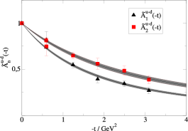
Figure 1: GFFs $\tilde{A}^{\mbox{\tiny u-d}}_{n0}(t)$ with $n=1,2$ for $\beta=5.6$, $\kappa_{\mbox{\tiny sea}}=\kappa_{\mbox{\tiny val}}=0.1560$. The form factors have been normalized to one at $t=0$ and fitted by a dipole form.

The domain-wall masses have been adjusted to keep the pseudoscalar lattice mass in the region of the lowest corresponding staggered one. For the Wilson fermion renormalization constants we use the perturbative one-loop results quoted in [7]. The renormalization constants for the domain-wall case are not yet calculated, so we use the tree-level value. Hence, our results are preliminary.

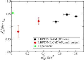
Figure 2: Axial coupling constant $g_{A}=\tilde{A}^{\mbox{\tiny u-d}}_{10}(0)$.

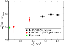
Figure 3: First moment of the spin-dependent parton distribution $\langle x\rangle_{\Delta u-\Delta d}=\tilde{A}^{\mbox{\tiny u-d}}_{20}(0)$.

We concentrate on the quark flavor combination u-d since the resulting matrix elements are free from disconnected contributions. The GFF $\tilde{A}^{\mbox{\tiny u-d}}_{10}(t)$ corresponds to the axial form factor, while $\tilde{A}^{\mbox{\tiny u-d}}_{20}(t)$ is the first GFF which is not directly accessible experimentally. Both GFFs are plotted with normalization $\tilde{A}^{\mbox{\tiny u-d}}_{n0}(0)=1$ for the heaviest quark mass in fig. 1. The curves provide dipole fits to the data points with the error bands representing one standard error. It is apparent that the dependencies on the parameters $x$ and $t$ of $\tilde{H}^{\mbox{\tiny u-d}}(x,\xi,t)$ do not factorize, a result that is very similar to the spin-independent case [8]. However, the difference between the two moments appears to be smaller in the spin-dependent case.

The axial coupling as a function of the quark mass is plotted in fig. 2. One should note, however, that this quantity is highly sensitive to finite-volume effects [9]. At least at the lightest mass, a couple of simulations at larger lattice volumes need to be performed to achieve a conclusive result for the chiral behavior.

The first moment of the forward parton distribution $\tilde{A}^{\mbox{\tiny u-d}}_{20}(0)$ is displayed in fig. 3. Although the measured values decrease in the chiral regime toward the experimental value, this result needs to be corroborated with better statistics.

4 CONCLUSIONS

In this talk we have presented first results on spin-dependent generalized parton distributions. In the forward case we have presented preliminary results for light quark masses which eventually should allow us to bridge the gap to the chiral regime.

While the axial coupling may be contaminated by substantial finite-size effects the first moment $\tilde{A}^{\mbox{\tiny u-d}}_{20}(0)$ of the spin-dependent GPD appears to be compatible with experiment in the chiral regime.

References

• [1] D. Müller, D. Robaschik, B. Geyer, F.M. Dittes and J. Horejsi, Fortsch. Phys.  42 (1994) 101. X.D. Ji, Phys. Rev. Lett.  78 (1997) 610. A.V. Radyushkin, Phys. Rev. D 56 (1997) 5524.
• [2] M. Diehl, arXiv:hep-ph/0307382.
• [3] V. Bernard, L. Elouadrhiri and U.G. Meissner, J. Phys. G 28 (2002) R1.
• [4] Y. Goto et al. [Asymmetry Analysis collaboration], Phys. Rev. D 62 (2000) 034017. M. Glück, E. Reya, M. Stratmann and W. Vogelsang, Phys. Rev. D 63 (2001) 094005. J. Blümlein and H. Böttcher, Nucl. Phys. B 636 (2002) 225.
• [5] M. Göckeler et al. [QCDSF Collaboration], arXiv:hep-ph/0304249. P. Hägler, J.W. Negele, D.B. Renner, W. Schroers, T. Lippert and K. Schilling [LHPC collaboration], Phys. Rev. D 68 (2003) 034505.
• [6] A. Hasenfratz and F. Knechtli, Phys. Rev. D 64 (2001) 034504.
• [7] D. Dolgov et al., Phys. Rev. D 66 (2002) 034506.
• [8] J.W. Negele et al., these proceedings, arXiv:hep-lat/0309060.
• [9] Th. Hemmert and A. Schäfer, private communication.