Investigations on the deconfining phase transition in QCD

Abstract

We investigate the deconfining phase transition in SU(3) pure gauge theory and in full QCD with two flavors of staggered fermions by means of a gauge invariant thermal partition functional. In the pure gauge case our finite size scaling analysis is in agreement with the well known weak first order phase transition. In the case of 2 flavors full QCD we find that the phase transition is consistent with weak first order, contrary to the expectation of a crossover for not too large quark masses.

1 INTRODUCTION

To detect the deconfinement phase transition in pure gauge theories the expectation value of the trace of the Polyakov loop is used as an order parameter. In presence of dynamical fermions the Polyakov loop ceases to be an order parameter since Z(N) symmetry is no longer a symmetry of the action. Alternatively deconfinement could be detected by looking at Abelian monopole condensation which can be detected [1] by means of the vacuum expectation value of a magnetically charged operator whose expectation value is different from zero in the confined phase and goes to zero at the deconfining phase transition.

In a different way, abelian monopole condensation can be signaled by the free energy needed to create an abelian monopole in the vacuum. This free energy can be computed [2, 3] through a gauge invariant lattice effective action which in turn is defined at zero temperature by means of the lattice Schrödinger functional and at finite temperature by means of a thermal partition functional. Since abelian monopole condensation is not related, as the Polyakov loop, to a symmetry of the lattice action, it could still be useful in order to detect a phase transition even if dynamical fermions are included into the action. The lattice thermal partition functional in presence of a static background field is defined [3, 4] as

$$\mathcal{Z}_{T}\left[\vec{A}^{\text{ext}}\right]=\int_{U_{k}(L_{t},\vec{x})=U_{k}(0,\vec{x})=U^{\text{ext}}_{k}(\vec{x})}\mathcal{D}U\,e^{-S_{W}}\,,$$ (1)

$T=1/aL_{t}$ is the physical temperature. T he spatial links belonging to the time slice $x_{t}=0$ are constrained to the value of the external background field,

$$U_{k}(x)|_{x_{t}=0}=U^{\text{ext}}_{k}(\vec{x})\,,\,\,\,\,\,(k=1,2,3)\,\,,$$ (2)

$U^{\text{ext}}_{k}(x)$ being the lattice version of the external continuum gauge field, the temporal links are not constrained. At finite temperature the relevant quantity is the free energy functional:

$$\frac{F[\vec{A}^{\text{ext}}]}{T_{\text{phys}}}=-\ln\frac{\mathcal{Z}_{T}[\vec{A}^{\text{ext}}]}{{\mathcal{Z}}_{T}[0]}\,.$$ (3)

When including dynamical fermions, the thermal partition functional in presence of a static external background gauge field, Eq. (1), becomes:

$$\begin{split}&\mathcal{Z}_{T}\left[\vec{A}^{\text{ext}}\right]=\\ &\quad=\int_{U_{k}(L_{t},\vec{x})=U_{k}(0,\vec{x})=U^{\text{ext}}_{k}(\vec{x})}\mathcal{D}Ue^{-S_{W}}\,\det M\,,\end{split}$$

where $S_{W}$ is the Wilson action and $M$ is the fermionic matrix. Notice that the fermionic fields are not constrained and the integration constraint is only relative to the gauge fields: this leads, as in the usual QCD partition function, to the appearance of the gauge invariant fermionic determinant after integration on the fermionic fields.

To detect monopole condensation we consider [2, 5] the following quantity defined in terms of free energy $F$ needed to create a monopole in the vacuum:

$$e^{-F/T_{\text{phys}}}=\frac{\mathcal{Z}_{T}\left[\vec{A}^{\text{ext}}\right]}{\mathcal{Z}_{T}[0]}\,.$$ (4)

In presence of monopole condensation $F$ is finite and $e^{-F/T_{\text{phys}}}\neq 0$. In practice it is easier to compute $F^{\prime}(\beta)$ the $\beta$-derivative of the free energy (eventually, since $F=0$ at $\beta=0$, $F$ can be obtained by numerical integration of $F^{\prime}(\beta)$).

2 SU(3) PURE GAUGE

We consider SU(3) pure gauge in an abelian monopole background field. The gauge potential in the continuum is

$$g\vec{b}^{a}({\vec{x}})=\delta^{a,3}\frac{n_{\mathrm{mon}}}{2}\frac{\vec{x}\times\vec{n}}{|\vec{x}|(|\vec{x}|-\vec{x}\cdot\vec{n})}\,,$$ (5)

where $\vec{n}$ is the direction of the Dirac string and $n_{\text{mon}}$ (integer) is the number of monopoles. On the lattice the spatial links exiting from the sites at the boundary of the time slice $x_{t}=0$ are constrained to the (lattice version of) the gauge potential Eq. (5). Links at spatial boundaries ($x_{t}\neq 0$) can be constrained to the monopole background field (“spatial fixed boundary conditions”) or can be periodic (“spatial periodic boundary conditions”). These two different choices (for the monopole field which vanishes at infinity) are equivalent in the thermodynamical limit. The simulations were performed on lattices of different spatial sizes ($16^{3}$, $24^{3}$, and $32^{3}$) and fixed the temporal extent ($L_{t}=4$), using APEmille/crate in Bari. We find that our data for $F^{\prime}(\beta,L_{s}^{\text{eff}})$ can be fitted according to the following scaling law

$$F^{\prime}(\beta,L_{s}^{\text{eff}})=\frac{a_{1}(L_{s}^{\text{eff}})^{\gamma}}{\left|(L_{s}^{\text{eff}})^{1/\nu}(\beta-\beta_{c})-d_{1}\right|^{\alpha}}\,,$$ (6)

where the above scaling relation holds quite well for a large range of the scaling variable $x=(L_{s}^{\text{eff}})^{1/\nu}(\beta-\beta_{c})$, with $\nu=0.334\pm 0.021$ consistent with a first order phase (see Fig. 1).

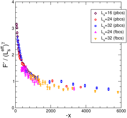
Figure 1: We plot together data for $F^{\prime}$ (fbcs: “spatial fixed boundary conditions”, $L_{s}^{\text{eff}}=L_{s}-2$) and (pbcs: “spatial periodic boundary conditions”, $L_{s}^{\text{eff}}=L_{s}$).

3 QCD ($N_{f}=2$)

We study QCD with two dynamical staggered fermions. We simulate the theory with a “cold” time-slice where (as in the case of pure gauge) the spatial links are constrained to the abelian monopole background field.

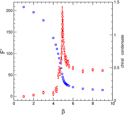
Figure 2: $F^{\prime}$ on a $16^{3}\times 4$ lattice in the case of full QCD with 2 dynamical flavors, is displayed together with chiral condensate.

In Fig. (2) the derivative of the free energy with respect to the gauge coupling $F^{\prime}(\beta)$ is displayed together with chiral condensate data suggest that the peak in $F^{\prime}(\beta)$ corresponds to the drop of the chiral condensate. Using our data for $F^{\prime}(\beta)$ on different spatial volumes and different bare quark masses we try to infer the critical behavior of two flavors full QCD near the phase transition. We varied the lattice size $L_{s}$ ($L_{s}=16,20,32$) and the staggered quark mass $m_{q}$ ($m_{q}=0.075,0.2676,0.5003$). At fixed $m_{q}$, as in the quenched case, the peak increases as the lattice volume is increased. At fixed spatial volume the critical coupling depends on $m_{q}$. All our lattice data can be described by a finite size scaling function where the gauge critical coupling now does depend on the quark mass and is determined by the chiral critical point[6, 7, 8]

$$\begin{split}&F^{\prime}(\beta,L_{s}^{\text{eff}},m_{q})=\\ &\quad\frac{a_{1}(L_{s}^{\text{eff}})^{\gamma}}{\left|(L_{s}^{\text{eff}})^{1/\nu}(\beta-\beta_{c}(0)-cm_{q}^{\eta})-d_{1}\right|^{\alpha}}\,,\end{split}$$ (7)

the relevant chiral critical exponents being compatible with those of the three-dimensional O(4) symmetric spin models [7]. We find that the critical exponent $\nu=0.31\pm 0.03$ is consistent with a first order phase transition, even though weaker than in SU(3) pure gauge (analogous indications have been obtained by the Pisa group [9]).

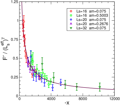
Figure 3: $F^{\prime}(\beta,L_{s}^{\text{eff}},m_{q})$ rescaled by the factor $(L_{s}^{\text{eff}})^{\gamma}$. The values of $L_{s}^{\text{eff}}$ and $m_{q}=am$ are displayed in the legend.

4 CONCLUSIONS

We investigated the phase transition in SU(3) pure gauge theory and in full QCD with two flavors of degenerate staggered fermions. To locate the phase transition we looked at the free energy to create a monopole in the vacuum. In the pure gauge case our finite size scaling analysis is consistent with the well known weak first order phase transition. In the case of QCD we find that the phase transition is compatible with a weak first order phase transition (contrary to the expectation of a crossover for not too large quark masses).

References

- [1] A. Di Giacomo et al., Phys. Rev. D61 (2000) 034503, hep-lat/9906024.
- [2] P. Cea and L. Cosmai, Phys. Rev. D62 (2000) 094510, hep-lat/0006007.
- [3] P. Cea and L. Cosmai, JHEP 11 (2001) 064.
- [4] P. Cea and L. Cosmai, JHEP 02 (2003) 031, hep-lat/0204023.
- [5] P. Cea and L. Cosmai, Nucl. Phys. Proc. Suppl. 94 (2001) 486, hep-lat/0010034.
- [6] F. Karsch and E. Laermann, Phys. Rev. D50 (1994) 6954, hep-lat/9406008.
- [7] J. Engels et al., Phys. Lett. B514 (2001) 299, hep-lat/0105028.
- [8] F. Karsch, E. Laermann and A. Peikert, Nucl. Phys. B605 (2001) 579, hep-lat/0012023.
- [9] J.M. Carmona et al., Phys. Rev. D66 (2002) 011503, hep-lat/0205025.