Numerical confirmation of analytic predictions for the finite volume mass gap of the XY-model

Abstract

Recent exact predictions for the massive scaling limit of the two dimensional XY-model are based on the equivalence with the sine-Gordon theory and include detailed results on the finite size behavior. The so-called step-scaling function of the mass gap is simulated with very high precision and found consistent with analytic results in the continuum limit. To come to this conclusion, an also predicted form of a logarithmic decay of lattice artifacts was essential to use for the extrapolation.

HU-EP-03/54

SFB/CCP-03-28

1 Introduction

For two-dimensional quantum field theories there are exact solutions available in quite a number of cases. The meaning of the notion ‘exact’ is however not quite universal. In many cases it does not imply a straight-forward evaluation, and often not rigorously provable conjectures are adopted at intermediate steps. To corroborate such solutions it is very attractive to compare — whenever possible — high precision numerical simulations with exact predictions. An interesting such opportunity arose in recent years from an exact solution of the famous XY-model [KosterlitzThouless73, Kosterlitz74] in its massive continuum limit taken from the vortex-phase. This solution involves a conjectured chain of equivalences that links it to the exactly solved sine-Gordon field theory [Zinn-Justin]. The predictions are particularly suitable for a numerical check since they include information about the XY-model in a finite volume and even about the asymptotic lattice spacing dependence for the standard discretization of the model. On the simulation side the XY-model profits from the practical absence of critical slowing down for cluster algorithms [Wolff89], allowing for large correlation lengths to be simulated, and from the availability of reduced variance estimators for correlations [Hasenbusch94_2].

Interesting light is shed on a problem inherent in all numerical lattice field theory computations, including QCD and asymptotically free two-dimensional models: the need of a continuum extrapolation. To carry it out, a theory based analytic form for the asymptotic dependence on the lattice spacing $a$ is required. Usually a power behavior $a$ and/or $a^{2}$ from Symanzik theory [Symanzik83], based on all-order perturbation theory, is used. In [Hasenfratz2000, Hasenbusch2001] high precision simulations of the $O(3)$-model revealed however that the expected $a^{2}$ behavior does not prevail down to very small lattice spacings, and at present there seems to be no theoretical understanding for this. The XY-model is not asymptotically free in the usual sense and the exact prediction for its $a$-dependence differs from the Symanzik behavior, which is very interesting to verify. A good understanding of the cut-off dependence is clearly important also for QCD simulations, in particular now that they become more and more precise and hence quantitatively useful for phenomenology.

2 Theoretical predictions

2.1 The LWW-coupling

The two dimensional nonlinear $O(2)$ symmetric $\sigma$-model can be defined by the classical Lagrangian

$$\mathcal{L}=\frac{1}{2g^{2}}\partial_{\mu}S^{a}\partial_{\mu}S^{a},\qquad S^{a}S^{a}=1,\qquad a=1,2\,.$$ (1)

When space-time is discretized the XY-model is recovered, its standard action being

$$S=-\beta\sum_{\langle k,l\rangle}\cos(\theta_{k}-\theta_{l})\,.$$ (2)

The summation is performed over all nearest neighbor pairs. The model describes a set of spins with unit length arranged on the sites of a square lattice that are subject to a ferromagnetic interaction. The angle $\theta_{n}$ denotes the alignment of the spin at site $n$ relative to an arbitrary axis and $\beta=1/g^{2}$ is the inverse temperature or bare coupling.

Let the spatial extent of the lattice be $L$. This introduces a natural external scale and renormalized couplings that run with $L$ can be defined. In [LWW91] the Lüscher-Weisz-Wolff-coupling (LWW) was introduced

$$\bar{g}^{2}(L)=2M(L)L\,.$$ (3)

Here $M(L)$ is the finite volume mass gap of the theory defined by the transfer matrix in the sector of zero spatial momentum. The running of the coupling is described by the $\beta$-function

$$\beta(\bar{g}^{2})=-L\frac{\partial\bar{g}^{2}}{\partial L}\,.$$ (4)

For finite scale changes the universal step-scaling function $\sigma$ has been defined, and it describes how the LWW coupling changes if the scale is dilated by a factor $s$

$$\sigma(s,\bar{g}^{2}(L))=\bar{g}^{2}(sL)\,.$$ (5)

The lattice version ($a$ is the lattice spacing) of the step scaling function $\Sigma(s,\bar{g}^{2},a/L)$ depends in addition on the resolution of the lattice.

2.2 DdV equation

Starting from the light-cone lattice regularization [DdV87, DdV89] of the sine-Gordon model and the corresponding Bethe Ansatz solution, a complete description of the exact spectrum of the model in finite volume is provided by the Destri-deVega (DdV) non-linear integral equations. They were originally suggested [DdV92, DdV95] for the ground state of the sine-Gordon or the closely related massive Thirring model, but can be systematically generalized to describe excited states as well; the (common) even charge sector of both models [DdV97, Feverati98, Feverati99] and the (different) odd charge sector in both sine-Gordon and massive Thirring model [Feverati98_2].

The ground state energy is given by

$$E_{0}(L)=-\frac{M}{\pi}\,{\rm Im}\int\limits_{-\infty}^{+\infty}\!\!dx\ \sinh(x+i\eta)\,\ln\left[1+e^{iZ_{0}(x+i\eta)}\right]\,.$$ (6)

The mass $M$ without an argument denotes here the infinite volume mass gap $M\equiv M(L=\infty)$. The parameter $\eta$ is needed to keep the branch of the logarithm well-defined. The result is independent of $\eta$ as long as $0<\eta<\pi$. The so-called counting function $Z_{0}(\theta)$ solves the nonlinear integral equation

$$\begin{split}Z_{0}(\theta)=&\ ML\sinh\theta\\ &-i\int\limits_{-\infty}^{+\infty}\!dx\ \left[G(\theta-x-i\eta)-G(\theta+x+i\eta)\right]\ln\left[1+e^{iZ_{0}(x+i\eta)}\right]\end{split}$$ (7)

with a kernel given by

$$G(\theta)=\frac{1}{2\pi}\int\limits_{-\infty}^{+\infty}\!\!dk\ e^{ik\theta}\ \frac{\sinh\frac{\pi k(p-1)}{2}}{2\,\cosh\frac{\pi k}{2}\sinh\frac{\pi kp}{2}}\,,$$ (8)

where $p=\beta^{2}_{\rm sG}/(8\pi-\beta_{\rm sG}^{2})$ parameterizes the sine-Gordon coupling $\beta_{\rm sG}$.

Similarly the energy of the first excited state is given by

$$E_{1}(L)=M-\frac{M}{\pi}\,{\rm Im}\int\limits_{-\infty}^{+\infty}\!\!dx\ \sinh(x+i\eta)\,\ln\left[1-e^{iZ_{1}(x+i\eta)}\right]\,,$$ (9)

with $Z_{1}(\theta)$ being a solution of

$$\begin{split}Z_{1}(\theta)=&\ ML\sinh\theta+\chi(\theta)\\ &-i\int\limits_{-\infty}^{+\infty}\!dx\ \left[G(\theta-x-i\eta)-G(\theta+x+i\eta)\right]\ln\left[1-e^{iZ_{1}(x+i\eta)}\right]\,.\end{split}$$ (10)

The source term $\chi(\theta)$ is of the form

$$\chi(\theta)=2\pi\,\int\limits_{0}^{\theta}\!\!dz\,G(z)$$ (11)

and $\eta$ is arbitrary within the same range as before.

The finite volume mass gap of the theory is $M(L)=E_{1}(L)-E_{0}(L)$. The XY-model is believed to lie in the same universality class as the sine-Gordon model with the sine-Gordon coupling $\beta_{\rm sG}=\sqrt{8\pi}$, or $p\to\infty$ [Zinn-Justin]. In this case the kernel simplifies to

$$G(\theta)=\frac{1}{2\pi}\int\limits_{-\infty}^{+\infty}\!\!dk\,\frac{e^{ik\theta}}{e^{\pi|k|}+1}\,.$$ (12)

The Fourier integral can be carried out

$$G(\theta)=\frac{1}{4\pi^{2}}\left(-\Psi(\frac{\pi-i\theta}{2\pi})-\Psi(\frac{\pi+i\theta}{2\pi})+\Psi(1-\frac{i\theta}{2\pi})+\Psi(1+\frac{i\theta}{2\pi})\right)$$ (13)

in terms of the digamma function $\Psi(z)$. Also the source term can be calculated exactly in the limit $p\to\infty$,

$$\begin{split}\chi(x+i\eta)=&-i\,\ln\left[\Gamma\left(\frac{1}{2}-\frac{ix-\eta}{2\pi}\right)\right]+i\,\ln\left[\Gamma\left(\frac{1}{2}+\frac{ix-\eta}{2\pi}\right)\right]\\ &+i\,\ln\left[\Gamma\left(1-\frac{ix-\eta}{2\pi}\right)\right]-i\,\ln\left[\Gamma\left(1+\frac{ix-\eta}{2\pi}\right)\right]\,.\end{split}$$ (14)

2.3 Asymptotic behavior

For large volumes ($L\to\infty$) and also for small volumes ($L\to 0$) asymptotic formulae exist which can be used to calculate the finite volume mass gap in this model independently of the DdV equation.

The $\beta^{2}_{\rm sG}\to 8\pi$ sine-Gordon model is equivalent to the $SU(2)$ symmetric chiral Gross-Neveu model and is thus asymptotically free. In principle it is straightforward to do perturbation theory for the XY-model using the formalism of Amit et al. [Amit79]. The final result, as usual in an asymptotically free model, is a power series in a running coupling. Technically however, the calculations are more involved than usual, since the perturbative contributions cannot be written in terms of usual Feynman integrals.

The 2-loop perturbative result for the LWW coupling is

$$\bar{g}^{2}=\frac{\pi}{2}(1+\gamma+u_{2}\gamma^{2})+\mathcal{O}(\gamma^{3})\,,$$ (15)

with the running coupling $\gamma$ solving

$$\frac{1}{2\gamma}-\frac{1}{2}\ln(2\gamma)=\ln\left(\frac{1}{ML}\right).$$ (16)

Along the lines described in [Amit79] we obtain

$$u_{2}=0.20(1),$$ (17)

where due to the complexity of the computation the 2-loop coefficient has to be obtained numerically in the end.

On the other hand, Lüscher has found a universal formula which describes the leading large volume corrections to the mass of the lightest particle on a spatial torus in terms of scattering amplitudes of the theory [Luescher86]. The formula exists in any dimension. It is particularly useful in two dimensional integrable models where the scattering amplitudes are known exactly. In our case it gives

$$\begin{split}\bar{g}^{2}=&2ML+\frac{2ML}{\pi}\int\limits_{-\infty}^{+\infty}\!\!d\theta\ \cosh\theta\,e^{-ML\cosh\theta}\left[1+e^{i\chi(\theta+\frac{i\pi}{2})}\right]\\ &+\mathcal{O}(e^{-2ML}).\end{split}$$ (18)

3 Numerical results

3.1 Numerical solution of the DdV equation

To calculate the finite volume mass gap $M(L)$ it is necessary to evaluate the nonlinear integral equations (7) and (10) numerically. The idea is to solve them iteratively [Ravanini2001]. In a first step the integral term on the right hand side is neglected, in every consecutive step the previous approximation is inserted into the integral. The iteration is aborted when the desired precision is reached. Further details of this procedure are described in [korzec2003]. Figure 1 shows some values of the LWW-coupling as a function of the the size in units of the infinite volume mass gap obtained from the numerical solutions of the DdV equations and compares them to the asymptotic formulas (15) and (18).

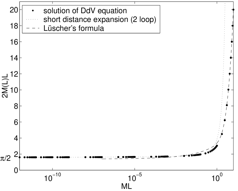
Figure 1: LWW coupling obtained from solutions of the DdV equation.

To compute the step-scaling function $\sigma(2,u)$ first a value $ML$ has to be found such that after solving the DdV equation for it $2M(L)L=u$ holds accurately enough. Then $\sigma$ is given by solving again with the doubled value $2ML$.

3.2 Monte Carlo study of the model

The XY-model can be simulated very effectively with cluster algorithms [Wolff89, Wolff88, Niedermayer97]. The finite volume mass gap may be obtained from the decay of the correlation function of spatially averaged spin fields (see [LWW91] for details). For our simulations we use a single cluster algorithm and an improved estimator for the correlation function [Hasenbusch94_2].

To calculate the step scaling function we perform calculations on lattices of different resolutions $a/L$. For each lattice a bare coupling $\beta$ is determined that leads to the desired value $u$ of the LWW-coupling. A simulation at the same bare coupling but with lattice size $2L/a$ yields a point of the lattice step-scaling function $\Sigma(2,u,a/L)$. To obtain the continuum step-scaling function it is necessary to perform a continuum extrapolation. The unusual form of the lattice artifacts in the XY-model was predicted in [Balog2000] and in the case of the step-scaling function reads

$$\Sigma(2,\bar{g}^{2},a/L)=\sigma(2,\bar{g}^{2})+\frac{c}{(\ln\xi+U)^{2}}+\mathcal{O}(\ln^{-4}\xi)\,,$$ (19)

where $U$ is a non-universal constant ($U=1.3(1)$ for the standard action [Balog2002]) and $c$ can be calculated for each $\bar{g}^{2}$ (see appendix A). The lattice resolution is expressed in terms of the infinite volume correlation length $\xi=\frac{1}{Ma}=\frac{L/a}{ML}$, which can be measured directly if it is not too large. When the bare coupling $\beta$ approaches $\beta_{c}$, the Kosterlitz Thouless (KT) theory [KosterlitzThouless73, Kosterlitz74] predicts the correlation length to diverge according to

$$\xi=A\exp\left(C\left|\frac{\beta_{c}-\beta}{\beta_{c}}\right|^{-\frac{1}{2}}\right)\,.$$ (20)

The non-universal constants are known with good precision for the standard action [Hasenbusch97],

$$A = 0.233\pm 0.003$$ (21)

$$C = 1.776\pm 0.004$$ (22)

$$\beta_{c} = 1.1199\pm 0.0001\,.$$ (23)

This result was derived in an approximative renormalization group study and is strictly valid only for $\beta\to\beta_{c}$. At $\beta\sim 1.05$ we see a numerical matching with KT, so we use eq. (20) to determine the correlation lengths yet closer to criticality. We emphasize that this result is only used for the lattice artifacts and that errors in $\xi$ are suppressed by the logarithm in (19).

Fitting the Monte Carlo estimates for the lattice step-scaling function to (19) yields a point of the continuum step scaling function and the constant $c$. Both values can be compared to predicted values, which is done for several values of the LWW-coupling in table 1. The small discrepancy between $c_{\rm th}$ and $c_{\rm MC}$ can presumably be attributed to subleading cutoff effects in the Monte Carlo data. Figure 2 illustrates the extrapolation for one of the points, the corresponding figures for the other points look qualitatively the same. Figure 3, which has an equally good $\chi^{2}$-value, demonstrates how important the knowledge of the lattice artifacts is. The data needed to extract these results are collected in table B of appendix B.

$\bar{g}^{2}$	$\sigma_{\rm DdV}(2,\bar{g}^{2})$	$\sigma_{\rm MC}(2,\bar{g}^{2})$	$c_{\rm th}$	$c_{\rm MC}$	$\chi^{2}/_{\rm dof}$
$3.0038$	$4.3895$	$4.40\phantom{0}\pm 0.02\phantom{0}$	$2.6176\pm 0.0002$	$2.4\pm 0.6$	$2.51/3$
$1.7865$	$1.8282$	$1.829\pm 0.007$	$5.30\phantom{00}\pm 0.01\phantom{00}$	$4.8\pm 0.5$	$0.73/3$
$1.6464$	$1.6515$	$1.657\pm 0.003$	$5.4\phantom{000}\pm 0.2\phantom{000}$	$4.3\pm 0.3$	$0.35/3$
$1.6020$	$1.6029$	$1.608\pm 0.004$	$5.5\phantom{000}\pm 1.5\phantom{000}$	$4.4\pm 0.5$	$0.90/3$

Table 1: At different values of the LWW-coupling theoretical predictions (DdV) for the step-scaling function are compared with numerical results (MC). Also the constant $c$ as predicted by theory (th) is compared to the numerical value.

\psfrag{tag1}{$(1.3+\ln\xi)^{-2}$}\psfrag{tag2}{$\Sigma(2,\bar{g}^{2}=1.7865,a/L)$}\psfrag{tag3}{MC-data}\psfrag{tag4}{solution of DdV equation}\psfrag{tag5}{linear fit}\includegraphics[width=433.62pt]{./images/u17865.eps}

Figure 2: Comparison of MC-data with a numerical solution of the DdV equation at $\bar{g}^{2}=1.7865$. The spatial extents $L/a$ of the lattices were $10,\ 20,\ 40,\ 80,\ 120$ and $160$. The smallest lattice was discarded in the fit.

\psfrag{tag1}{$a/L$}\psfrag{tag2}{$\Sigma(2,\bar{g}^{2}=1.7865,a/L)$}\psfrag{tag3}{MC-data}\psfrag{tag4}{solution of DdV equation}\psfrag{tag5}{polynomial fit}\includegraphics[width=433.62pt]{./images/u17865w.eps}

Figure 3: Comparison of MC-data with a numerical solution of the DdV equation at $\bar{g}^{2}=1.7865$. The predicted continuum value could not have been confirmed by an extrapolation with a second degree polynomial (including a linear term), as used in this plot.

4 Conclusions

In this work we have found a remarkable consistency between analytic and numerical results. For several values of the LWW coupling we found perfect agreement between numerical continuum-extrapolated values of the step scaling function and those following from solving the DdV equation. This agreement is only obtained by employing for the extrapolation a logarithmic dependence on the lattice spacing that follows from the connection between the sine-Gordon and the XY-model together with the KT-behavior of the correlation length close to the critical point.

This overall consistency furnishes strong evidence that all the considerations and assumptions leading from the six-vertex model via Bethe Ansatz to a set of integral equations that can be used to calculate the energy spectrum of the sine-Gordon model are correct. Simultaneously it also corroborates the assertion that the massive continuum limit of the lattice XY-model can be described by the $\beta^{2}_{\rm sG}\to 8\pi$ limit of the continuum sine-Gordon model. In Ref. [Balog2002] the latter was investigated by the Form Factor Bootstrap construction. The renormalized 4-point coupling $g_{\rm R}$ and 2-point correlation functions were compared to their lattice counterparts. Similarly to our findings here, after (and only after) the logarithmic lattice artifacts were taken into account, non-trivial agreement between lattice data and Form Factor results was found.

Indirectly also the KT-scenario is confirmed once more. Calculations leading to this scenario are more or less approximate and there has been a controversy whether they can be trusted or not for a long time [Luther77]. This result demonstrates in an impressive way, how important it is to have theory-based information on the functional form of lattice artifacts in order to extract the right continuum values from numerical data. Although the accessible range of lattices is much bigger and the precision higher than it would be in four dimensional theories, an extrapolation to the continuum could lead to uncontrolled systematic errors for precise data, if the right form of the lattice artifacts were not known.

Acknowledgement. We would like to thank Burkhard Bunk for discussions. This investigation was supported in part by the Hungarian National Science Fund OTKA (under T034299 and T043159) and by the German science foundation DFG in Graduiertenkolleg GK271 and SFB/TR9.

Appendix A Lattice artifacts of the step-scaling function

The LWW-coupling $\bar{g}^{2}=2M(L)L$ on a lattice is affected by lattice artifacts. In contrast to the simulations we now consider families of lattice calculations at fixed physical volume in units of the infinite volume mass gap, that is fixed $ML$. Then each chosen resolution $a/L$ in principle fixes a value for $\beta$ and hence also $\bar{g}^{2}$. In this sense we find $\bar{g}^{2}=f(ML,\xi)$, where $\xi=(Ma)^{-1}$ is used. The leading $\xi$-dependence is predicted by theory [Balog2000] to be

$$f(ML,\xi)=f_{0}(ML)-\frac{f_{1}(ML)\pi^{2}}{2(\ln\xi+U)^{2}}+\mathcal{O}([\ln\xi]^{-4}),\quad f_{0}(ML)=f(ML,\infty)$$ (24)

where $U$ is an action dependent constant ($U\approx 1.3$ for the standard action) and $f_{1}(ML)$ a coefficient. In solving the DdV equation (see figure 1) we evaluated $f_{0}(ML)$. In [Balog2000] it was shown that the same function $f_{1}$ also characterizes the approach of the the sine-Gordon model to its XY-model limit. Here one may also define an LWW coupling $\bar{g}^{2}_{\rm sG}$ and study its dependence on $p$ for fixed $ML$ to derive

$$\bar{g}^{2}_{\rm sG}=\tilde{f}(ML,p)=f_{0}(ML)+\frac{2f_{1}(ML)}{p^{2}}+\mathcal{O}(p^{-4})$$ (25)

for large $p$. This relation is entirely in the continuum and it hence becomes clear that $f_{1}$ is universal.

Numerically we avoid reference to infinite volume quantities (except here for the artifacts) and determine the step-scaling function $\sigma(2,\bar{g}^{2})$ at a certain fixed $\bar{g}^{2}=u$. The relation to the present language is

$$\sigma(2,u)=f_{0}[2f_{0}^{-1}(u)],$$ (26)

where $f_{0}^{-1}$ is the inverse function of $f_{0}$. At finite $\xi$ a computable slightly different value $(M+\delta M)L$ is associated with the target $u$-value. Then the doubled value is mapped to $\Sigma$ instead of $\sigma$. Collecting now all these corrections to leading order we obtain

$$\Sigma(2,u,a/L)-\sigma(2,u) = \left(\frac{2f_{0}^{\prime}(2ML)}{f_{0}^{\prime}(ML)}f_{1}(ML)-f_{1}(2ML)\right)\frac{\pi^{2}}{2(\ln\xi+U)^{2}}$$ (27)

$$= c(ML)\;\frac{1}{(\ln\xi+U)^{2}}$$

which defines $c(ML)$.

Further corrections to (27) are of order $\mathcal{O}([\ln\xi]^{-4})$. The required derivatives of $f_{0}$ in the continuum can be obtained numerically from solutions of the DdV equation. Also the coefficient $f_{1}$ may be gained from a numerical solution of the sine-Gordon version of the DdV equations. Instead of using the XY-model specific integral kernel (13) the version (8) with finite $p$ is taken. All data needed to calculate $c$ is collected in table LABEL:DdVtable.

Appendix B Tables

In the following two tables some of the data is collected that is needed to extract the results. An estimate of the derivative $\frac{\partial\Sigma}{\partial\bar{g}^{2}}$ is used to propagate into the total error of $\Sigma$ the statistical error of $\bar{g}^{2}$ and to correct the value of $\Sigma$ for the small difference between $u$ and $\bar{g}^{2}$. In most cases this correction amounts to a small shift compared with the statistical errors. The results in table LABEL:DdVtable were obtained twice independently.

$L/a$	$\phantom{0}\beta$	$\phantom{0}\bar{g}^{2}(L)$	$\bar{g}^{2}(2L)$	$\phantom{0}u$	$\Sigma(2ua/L)$
$20$	$0.9649$	$3.0022(45)$	$4.5144(74)$	$3.0038$	$4.519(13)$
$40$	$1.0000$	$3.0036(41)$	$4.4824(75)$	$3.0038$	$4.483(12)$
$80$	$1.0241$	$3.0146(39)$	$4.5055(76)$	$3.0038$	$4.480(12)$
$120$	$1.0359$	$2.9919(39)$	$4.4232(64)$	$3.0038$	$4.451(11)$
$160$	$1.0423$	$3.0069(38)$	$4.4742(64)$	$3.0038$	$4.466(11)$
$10$	$1.0358$	$1.7866(16)$	$1.9379(19)$	$1.7865$	$1.9378(31)$
$20$	$1.0541$	$1.7837(16)$	$1.9161(19)$	$1.7865$	$1.9222(40)$
$40$	$1.0668$	$1.7860(16)$	$1.9010(19)$	$1.7865$	$1.9019(35)$
$80$	$1.0756$	$1.7896(16)$	$1.8973(19)$	$1.7865$	$1.8911(37)$
$120$	$1.0800$	$1.7882(17)$	$1.8898(19)$	$1.7865$	$1.8869(38)$
$160$	$1.0830$	$1.7850(16)$	$1.8778(13)$	$1.7865$	$1.8796(21)$
$20$	$1.0758$	$1.64585(73)$	$1.71173(79)$	$1.6464$	$1.7125(12)$
$40$	$1.0844$	$1.64632(75)$	$1.70116(83)$	$1.6464$	$1.7013(16)$
$80$	$1.09076$	$1.64646(73)$	$1.69317(81)$	$1.6464$	$1.6931(13)$
$120$	$1.0937$	$1.64636(74)$	$1.68885(79)$	$1.6464$	$1.6889(13)$
$160$	$1.09551$	$1.64645(77)$	$1.68774(80)$	$1.6464$	$1.6877(13)$
$10$	$1.0720$	$1.5971(12)$	$1.6721(66)$	$1.602$	$1.6801(69)$
$20$	$1.0825$	$1.6033(12)$	$1.6574(13)$	$1.602$	$1.6556(21)$
$40$	$1.0903$	$1.6032(12)$	$1.6463(14)$	$1.602$	$1.6449(20)$
$80$	$1.0960$	$1.6020(11)$	$1.6397(13)$	$1.602$	$1.6397(20)$
$120$	$1.0984$	$1.6034(13)$	$1.6365(14)$	$1.602$	$1.6349(20)$
$160$	$1.1000$	$1.6028(13)$	$1.6330(13)$	$1.602$	$1.6321(20)$

Table 2: Sim