KANAZAWA-03-23     
ITEP-LAT-2003-18     
Energy-entropy study of projected space–like monopoles
in finite–T quenched SU(2) QCD

Abstract

Properties of space–like monopoles projected on the 3D space in finite temperature quenched SU(2) QCD are studied. The monopole energy is derived from the effective action of the monopoles which is determined by an inverse Monte-Carlo method. Then the entropy is fixed with the help of the monopole–loop distribution.

1 INTRODUCTION

The dual superconductor mechanism [1] of color confinement is confirmed in many numerical simulations in the Maximal Abelian (MA) gauge [2] (for a review, see Ref. [3]). This mechanism is based on the existence of the Abelian monopoles which are condensed in the confinement phase of QCD [4, 5]. The monopole condensate corresponds to the so-called percolating (infrared) cluster [6, 7] of the monopole trajectories. The tension of the confining string gets a dominant contribution from the IR cluster [7] while the finite-sized (ultraviolet) clusters do not play any role in confinement. Various properties of the UV and IR monopole clusters were studied previously in Refs. [7, 8, 9].

In the high temperature phase the monopoles become static. In this phase the IR cluster disappears [6, 7] and, consequently, the confinement of the static quarks is absent because only spatial components of the IR monopole cluster are relevant for the confinement. We investigate the action, the length distribution and the entropy of spatial components of the infrared monopole clusters following Ref. [9].

2 MODEL

We use the Wilson action, $S(U)=-\frac{\beta}{2}\,{\mathrm{Tr}}U_{P}$, to generate 1000-3000 configurations of the SU(2) gauge field, $U$, for $\beta=2.3\sim 2.6$ on $48^{3}\times N_{t}$, $N_{t}=6,8,12,16$ lattices. Performing the MA gauge fixing, we locate Abelian monopoles in the gluonic fields configurations in a standard way. The phase of the diagonal component of the SU(2) gauge field gives the Abelian gauge field, $\theta_{\mu}(s)=\arg\,U^{11}_{\mu}(s)$. Then we construct the Abelian field strength, $\theta_{\mu\nu}(s)\in(-4\pi,4\pi)$, which is decomposed into two parts, $\theta_{\mu\nu}(s)=\bar{\theta}_{\mu\nu}(s)+2\pi m_{\mu\nu}(s)$. Here $\bar{\theta}_{\mu\nu}(s)\in[-\pi,\pi)$ and $m_{\mu\nu}(s)$ are the electromagnetic flux and the Dirac string coming through the plaquette $P_{\mu\nu}(s)$, respectively. The ends of the Dirac strings correspond to the conserved elementary monopole currents [10], $k_{\mu}(s)=1/2\epsilon_{\mu\nu\rho\sigma}\partial_{\nu}m_{\rho\sigma}(s+\hat{\mu})\in{Z\!\!\!Z}$, where $\partial$ is the forward lattice derivative. The elementary monopoles are defined on the fine lattice with the spacing $a$. To study the monopole charges at various scales $b=na$, we use the extended $n^{3}$ monopole construction [6],

$$k_{\mu}^{(n)}(s)=\!\!\sum_{i,j,l=0}^{n-1}\!\!k_{\mu}(ns+(n-1)\hat{\mu}+i\hat{\nu}+j\hat{\rho}+l\hat{\sigma}).$$

The spatially projected currents are:

$$K_{i}^{(n)}(\vec{s})=\sum\nolimits^{N_{t}-1}_{s_{4}=0}\,k_{i}^{(n)}(s,s_{4})\,,\,\,i=1,2,3\,.$$ (1)

3 MONOPOLE ACTION

The monopole action of the $3D$ projected IR monopole clusters can be defined using the inverse Monte–Carlo method [4]. The action is represented in a truncated form [4, 11] as a sum of the $n$–point ($n\geq 2$) operators $S_{i}$:

$$S_{{\mathrm{mon}}}[k]=\sum\nolimits_{i}f_{i}S_{i}[k]\,,\vspace{-2mm}$$

where $f_{i}$ are the coupling constants. Following Ref. [9] we adopt only the two–point interactions in the monopole action ($i.e.$ interactions of the form $S_{i}\sim k_{i}(s)k_{j}(s^{\prime})$).

Figure 1: The parameter $f_{0}$ $vs.$ $b$ at $T=0.8T_{c}$.

Similarly to the $4D$ case we find that the monopole action of the $3D$ currents is proportional with a good accuracy to the length of the monopole loop, $S_{{\mathrm{mon}}}=f_{0}L+const$. The coupling $f_{0}$ shows a good scaling in agreement with Ref. [4], as can be seen from Fig. 1 where this coupling is shown as a function of the scale $b$ at $T=0.8T_{c}$.

4 LENGTH DISTRIBUTION

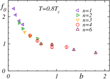
The length of the $4D$ IR monopole currents in the finite volume $V$ is distributed according to the Gaussian law [9]:

$$D^{IR}(L)\propto\exp\{-\alpha(b,V)L^{2}+\gamma(b,T)L\}\,.$$ (2)

The length distribution function, $D(L)$, is proportional to the weight with which the particular trajectory of the length $L$ contributes to the partition function. In Eq. (2) we neglect a power-law prefactor which is essential for the distribution of the ultraviolet clusters.

Since the monopole density, $\rho_{IR}=L_{max}/V$, is finite, the peak of the distribution (2), $L_{max}=\gamma(b,T)/2\,\alpha(b,V)$, must be proportional to the volume of the system for large volumes. Thus, in the thermodynamic limit we expect $\alpha(b,V)=A(b)/V$, where $A(b)$ is a certain function. Therefore in the thermodynamic limit the parameter $\alpha$ vanishes.

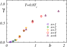
Apart from the finite–volume effect, the distribution (2) has contributions from the energy and the entropy. As seen above, the action contribution is proportional to $e^{-f_{0}L}$. The entropy contribution is proportional to $\mu^{L}$ (with $\mu>0$) for sufficiently large monopole lengths, $L$. Thus, the entropy factor, $\mu$, is

$$\mu=\exp\{f_{0}+\gamma\}\,.$$ (3)

Since we are performing the simulations in a finite volume we fit numerically obtained distributions of the $3D$ projected currents by the function (2) and then use the bootstrap method to estimate the statistical errors. We find that the parameter $\gamma$ shows a good scaling with $b$. An example at $T=0.8T_{c}$ is shown in Fig. 2. In a small $b$–region we find that $\gamma\propto b^{\eta}$ with $\eta\sim 3$ for low temperatures, say, at $T\sim 0.5T_{c}$, whereas $\eta\sim 2$ for $T\to T_{c}$.

Figure 2: The parameter $\gamma$ $vs.$ $b$ at $T=0.8T_{c}$.

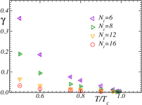
At the critical temperature, $T=T_{c}$, the $4D$ IR monopole cluster disappears and we expect a similar behaviour for the $3D$ projected IR cluster. Thus the parameter $\gamma(b,T)$ should vanish at the critical point. This is indeed the case according to Fig. 3 which shows $\gamma$ for elementary ($n=1$) monopoles as a function of temperature for various temporal extensions of the lattice.

Figure 3: The parameter $\gamma$ $vs.$ $T$ for $n=1$.

5 MONOPOLE ENTROPY

We determine the entropy using Eq. (3). The numerical results for the entropy factor $\mu(b,T)$ are shown in Fig. 4 for various temperatures.

Figure 4: The entropy factor $\mu$ $vs.$ the scale $b$ at temperatures $T/T_{c}=0.8,0.9$ and $0.99$.

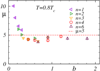
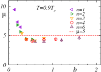
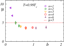
If the monopoles are randomly walking on a $3D$ hypercubic lattice then we should get $\mu=5$ since five choices exist at each site for the monopole current to go further. Note that $\mu>5$ for small values of $b$ because in this region the quadratic monopole actions are not enough [11].

At large $b$ the entropy factor tends to a fixed value around 4, which seems independent of temperature. Contrary to the $4D$ case [9] the entropy $\mu$ for projected monopoles does not approach unity in the $b\to\infty$ limit. Thus we observe that the spatially projected monopole currents exhibit a motion close to the random walk at non–zero temperatures.

References

- [1] G. ’t Hooft, in High Energy Physics, ed. A. Zichichi, EPS International Conference, Palermo (1975); S. Mandelstam, Phys. Rept. 23 (1976) 245.
- [2] A. S. Kronfeld et al, Phys. Lett. B 198, 516 (1987); Nucl. Phys. B 293, 461 (1987).
- [3] T. Suzuki, Nucl. Phys. Proc. Suppl. 30 (1993) 176; M. N. Chernodub, M. I. Polikarpov, hep-th/9710205; R.W. Haymaker, Phys. Rept. 315 (1999) 153.
- [4] H. Shiba, T. Suzuki, Phys. Lett. B 351 (1995) 519; N. Arasaki et al, Phys. Lett. B 395 (1997) 275.
- [5] M.Chernodub, M.I.Polikarpov, A.I.Veselov, Phys.Lett.B 399 (1997) 267; Nucl. Phys. Proc. Suppl. 49 (1996) 307;
- [6] T.L. Ivanenko, A.V. Pochinsky, M.I. Polikarpov, Phys. Lett. B 252 (1990) 631.
- [7] S. Kitahara, Y. Matsubara, T. Suzuki, Progr. Theor. Phys. 93 (1995) 1.
- [8] A. Hart, M. Teper, Phys. Rev. D58 (1998) 014504; P.Y. Boyko, M.I. Polikarpov, V.I. Zakharov, hep-lat/0209075; M. N. Chernodub, V. I. Zakharov, Nucl. Phys. B669 (2003) 233; V. G. Bornyakov et al, hep-lat/0305021.
- [9] M. N. Chernodub, et al, hep-lat/0306001; hep-lat/0308004.
- [10] T. A. DeGrand, D. Toussaint, Phys. Rev. D 22 (1980) 2478.
- [11] M. N. Chernodub et al, Phys. Rev. D 62 (2000) 094506; hep-lat/9902013.