Dynamical fermions by global acceptance steps

Abstract

A study of principle is conducted on the inclusion of the fermionic determinant as a Metropolis acceptance correction. It is carried out in the 2-D Schwinger model to prepare later applications to the Schrödinger functional. A mixed stochastic/determistic acceptance step is found that allows to include some problematic modes in a way to avoid the collapse of the acceptance rate due to fluctuations.

1 Introduction

The inclusion of light dynamical fermions in a formerly quenched simulation boosts the computational demand by a very large factor for standard Hybrid Monte Carlo (HMC) type algorithms. This is even true in cases like the Schrödinger functional at weak coupling (small physical volume), where we expect the fermionic determinant to be less influential. We here explore the naive idea to propose in such cases gauge configurations by an effcient pure gauge update scheme and to filter these proposals by an accept reject step that leads to the correct full QCD ensemble. Although it is advantageous to optimize the coupling or even the type of action to be used for the proposals, we here focus on the case of proposing with just the gauge part of the full action. A more detailed account is given in [1].

We use the two-flavour two-dimensional Schwinger model with a non-compact lattice gauge field as a test-case with the partition function

$$Z=\int D\mu(A)\,|\det(D_{W}+m)|^{2},$$ (1)

where $D_{W}$ is the Wilson Dirac operator. The gauge action is included in the normalized measure

$$D\mu(A)\propto\prod_{x\mu}dA_{\mu}(x)\,\prod_{\mu}\delta\bigl{(}\sum_{x}A_{\mu}\bigr{)}\;\mbox{\rm e}^{-S_{G}-S_{\xi}}\\$$ (2)

where $S_{G}$ is the plaquette action and

$$S_{\xi}=\frac{1}{2\xi^{2}}\sum_{x}(\Delta^{*}_{\mu}A_{\mu})^{2}$$ (3)

a gauge fixing term with the backward difference operator $\Delta^{*}_{\mu}$. Periodic boundary conditions are assumed and the $\delta$-function eliminates the integration over two zero-momentum modes. In $D_{W}$ the compact gauge variables $U_{\mu}=\exp(igA_{\mu})$ and with them the coupling strength $g$ enter. In the following it is replaced by the dimensionless variable $z=\sqrt{\sigma}L$, where $\sigma=g^{2}/2$ is the string tension. The gauge part of the action is purely Gaussian. Gauge fields distributed according to $D\mu(A)$ can be generated in momentum space and then Fourier transformed. This amounts to an ideal independent sampling or global heatbath algorithm. In Fig.1 the unquenched

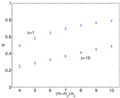
Figure 1: Acceptance with the exact determinant, $L=16$.

Metropolis acceptance rate

$$q = \frac{1}{Z}\int D\mu(A)\int D\mu(A^{\prime})$$

$$|\det(D_{W}+m)|^{2}\,w(A,A^{\prime})$$

with

$$w(A,A^{\prime})=\min\left(1,\frac{|\det(D^{\prime}_{W}+m)|^{2}}{|\det(D_{W}+m)|^{2}}\right)$$ (5)

is shown for such proposals as a function of the mass. The determinants have been evaluated exactly in this case (data with error bars). The critical mass is defined from the spectral gap for individual configurations and $m_{c},\sigma_{c}^{2}$ are its mean and variance with respect to $D\mu(A)$. For the range shown no execptional configurations are proposed in practice. The circles in the plot are obtained by assuming a Gaussian distribution for the fermionic part of the action, measuring its width and evaluating $q$ analytically for this model. Although the cost to compute exact determinants in higher dimension is prohibitive we here see that good acceptance of our global correction is possible. In [1] it is shown that $q$ is actually an upper bound for the stochastic method discussed next.

2 Stochastic acceptance steps

An independent new configuration $A^{\prime}$ proposed as a successor to $A$ is now accepted with the probability

$$w_{0}(A,A^{\prime};\eta)=\min[1,\rho(M\eta)/\rho(\eta)]$$ (6)

where $\eta$ is a pseudofermionic random field generated with some distribution $\rho$ (typically Gaussian) and $M=(D_{W}^{\prime}+m)^{-1}(D_{W}+m)$ is the ‘ratio’-operator. The main cost of this step is just an inversion. It leads to a correct algorithm due to detailed balance holding on average,

$$|\det(D_{W}+m)|^{2}\left<w_{0}(A,A^{\prime};\eta)\right>_{\eta} =$$

$$|\det(D_{W}^{\prime}+m)|^{2}\left<w_{0}(A^{\prime},A;\eta)\right>_{\eta}$$ , (7)

which is shown by a change of variables in the $\eta$-integral. As mentioned before

$$\langle w_{0}\rangle_{A,A^{\prime},\eta}=q_{0}\leq q$$ (8)

has been derived. It turns out that for most of the physical situations shown in Fig.1 the value of $q_{0}$ is smaller than $q$ to such an extent that the stochastic algorithm is rendered useless. We found that this is related to the spectrum of $M^{\dagger}M$ whos eigenvalues $\lambda_{i}$ also occur in the generalized problem with $(D_{W}+m)(D_{W}+m)^{\dagger}$ on one side and its primed companion on the other. Full spectra are easily computed in our model and typically show a structure of two pairs of eigenvalues of order $g^{2},g^{-2}$ respectively and the bulk of the spectrum near one. The occurence of these special modes can be understood in perturbation theory. By analytically computing $\left<w_{0}(A,A^{\prime};\eta)\right>_{\eta}$ as a function of $\{\lambda_{i}\}$ one sees that these extremal eigenvalues spoil the stochastic acceptance, even if $\prod\lambda_{i}\approx 1$ and $q$ is close to one, and then lead to $q_{0}$ being very much smaller than $q$. As a remedy to this problem we found that detailed balance also holds exactly [1] for a partially stochastic (PSD) estimation of the determinant ratio with the acceptance probability

$$w_{4}(A,A^{\prime})=$$ (9)

$$\min\left[1,\prod_{i\in S}\lambda_{i}^{-1}\exp(-\eta^{\dagger}\bar{P}(M^{\dagger}M-1)\bar{P}\eta)\right].$$

Here $S$ is the index set corresponding to the four extremal eigenvalues $\lambda_{i}$ (two from either end of the spectrum) that caused the trouble. The complement of the span of the corresponding eigenvectors defines the projector $\bar{P}$. Instead of four also any other even number of extremal eigenvalues may be taken symmetrically from both ends of the spectrum, and then this family of algorithms interpolates between the exact determinant $w$ and the fully stochastic method with $w_{0}$. A few extremal generalized eigenvalues and -vectors may for instance be computed with Lanczos or Ritz minimization methods, but this point needs further study.

Results for acceptance rates are found in Figs.2 and 3.

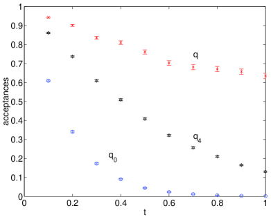
Figure 2: Acceptance vs. stepsize $t$ ($z=2,L=8,m=m_{c}+5\sigma_{c},\xi=0$).

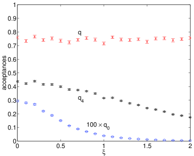
Figure 3: Acceptance vs. gaugeparameter $\xi$ ($z=1,L=8,m=m_{c}+8\sigma_{c},t=1$).

Here a free parameter $t$ has been introduced, that allows so vary the size of proposed moves $A\to A^{\prime\prime}=\cos(\pi t/2)A+\sin(\pi t/2)A^{\prime}$ with $A^{\prime}$ generated by global heatbath. Also these proposals obey detailed balance with respect to the gauge action. Fig.2 demonstrates that for larger $t$-values PSD remains a feasible algorithm. As long as the gauge parameter $\xi$ vanishes, simulated fields occur in a completely fixed gauge, while for growing $\xi$ the proposals are positioned more and more randomly on their gauge orbits. Fig.3 shows as one may intuitively expect that this freedom of gauge mismatch lowers the acceptance rate. Note that $q$ with the exact determinant is independent of $\xi$. For a locally gauge invariant distribution $\rho$ the $\eta$-averages of $w_{0}$ and $w_{4}$ are invariant under transforming both $A$ and $A^{\prime}$ with the same gauge function due to the gauge covariance of $D_{W}$ but not under gauge moves of $A^{\prime}$ relative to $A$. Hence the acceptance rate and autocorrelation times are $\xi$-dependent although physical results are not.

3 Conclusions

We found that at least in the 2-D Schwinger model the inclusion of fermions by a global accept step is possible. Gauge fields in this superrenormalizable model are generally smoother than in QCD and this is probably important for the success of the method. In sufficiently small physical volume with Schrödinger functional boundary conditions however a similar situation arises. We hope to be able to apply the global acceptance method there and maybe find an efficiency superior to HMC. This method has already found 4-D applications with blocked and hence smoother gauge fields entering into the Dirac operator [2, 3]. Here the use of HMC seems too complicated due to the complex dependence of the fermion action on the fundamental (unblocked) gauge fields. Also for such applications it seems to be valuable to understand the behaviour of the acceptance rate in detail and to look for tricks to boost it.

References

- [1] F. Knechtli and U. Wolff, Nucl. Phys. B663 (2003) 3, hep-lat/0303001.
- [2] A. Hasenfratz, (2002), hep-lat/0211007.
- [3] A. Hasenfratz and F. Knechtli, Comput. Phys. Commun. 148 (2002) 81, hep-lat/0203010.