Determination of monopole condensate from monopole action
in quenched SU(2) QCD

Abstract

We study the effective monopole action obtained in the Maximal Abelian projection of quenched SU(2) lattice QCD. We determine the quadratic part of the lattice action using analytical blocking from continuum dual superconductor model to the lattice model. The leading contribution to the quadratic action depends explicitly on value of the monopole condensate. We show that the analytical monopole action matches the numerically obtained action in quenched SU(2) QCD with a good accuracy. The comparison of numerical and analytical results gives us the value of the monopole condensate in quenched SU(2) QCD, $\eta=243(42)$ MeV.

I Introduction

The dual superconductor mechanism DualSuperconductor is one of the most promising mechanisms invented to explain the confinement of color in non–Abelian gauge theories. The basic element of this mechanism is the existence of specific field configurations – called Abelian monopoles – in the QCD vacuum. The monopoles are identified with the help of the Abelian projection method AbelianProjections , which uses the partial gauge fixing of the SU(N) gauge symmetry up to an Abelian subgroup. The Abelian monopoles appear naturally in the Abelian gauge as a result of the compactness of the residual Abelian group.

Various numerical simulations indicate that the Abelian monopoles may be responsible for the confinement of quarks (for a review, see, $e.g.$, Ref. Reviews ). The Abelian monopoles provide a dominant contribution to the tension of the fundamental chromoelectric string AbelianDominance ; shiba:string ; koma:string . In Ref. MonopoleCondensation it was qualitatively shown that the monopole condensate is formed in the low temperature (confinement) phase and it disappears in the high temperature (deconfinement) phase. The energy profile of the chromoelectric string as well as the field distribution inside it can be described with a good accuracy by the dual superconductor model string:profile ; koma:string ; ref:koma:suzuki

There were various attempts to determine the dual lagrangian and the values of its couplings ref:suzuki:maedan ; baker ; various:attempts ; ref:bali:string ; singh ; string:profile ; ref:koma:suzuki . A simplest version of the dual superconductor model for SU(2) gauge theory contains three independent parameters: the mass of the monopole, $M_{\Phi}$, the monopole charge, $g$, and the value of the monopole condensate, $\eta$. In Ref. string:profile the SU(2) string profile was compared with the classical string solution of the dual superconductor in continuum and the mass of the dual gauge boson, $M_{B}=g\eta$, and the monopole mass were shown to be equal, $M_{B}\approx M_{\Phi}\approx 1.3$ GeV. These values are close to the results of other groups.

The value of the monopole condensate derived from the chromoelectric string analysis of Ref. string:profile is $\eta=194(19)$ MeV. In this paper we determine the value of the monopole condensate from the effective monopole action obtained in the numerical simulations of quenched SU(2) QCD. Our strategy is the following. We relate the lattice monopole model on the lattice with the continuum dual superconductor model using the approach of blocking of the continuum variables to the lattice proposed in Ref. BlockingOfFields . Generally, this method allows to construct perfect lattice actions and operators in various field theories. In particular, this method was used in Ref. ref:ishiguro:suzuki:chernodub for the quenched SU(2) QCD at high temperatures to study the dynamics of the static monopoles. The lattice monopole action obtained with the help of such a blocking depends on the parameters of the original continuum model. The comparison of the analytical form of the lattice monopole action with the corresponding numerical results allows in general to fix the parameters of the continuum model. In this paper we concentrate on the determination of the monopole condensate in the quenched SU(2) QCD in the Maximal Abelian projection kronfeld .

The plan of the paper is the following. In Section II we propose the method of blocking from continuum to the lattice of the monopole currents in four dimensional space–time. We compute the quadratic part of the monopole action analytically in Section III, while the numerical computation is done in Section IV. In Section V we compare the numerical data with analytically calculated action and fix the value of the monopole condensate. Our conclusions are presented in the last Section.

II Blocking from continuum in four dimensions

The method of blocking of continuum variables to the lattice BlockingOfFields ; ref:ishiguro:suzuki:chernodub constructs the lattice model (at given finite lattice spacing $b$) starting from a model in continuum. The essence of this method is simple. Consider, for example, the blocking of the topological variables, such as the monopole charge in three space–time dimensions ref:ishiguro:suzuki:chernodub . In $3D$ the monopoles are instantons characterized by their positions and the magnetic charges. Suppose, that the dynamics of these monopole charges in continuum is described by a Coulomb gas model with two parameters, the fugacity, $\zeta$, and the monopole charge, $g$. Let us superimpose a cubic lattice with the lattice spacing $b$ on a particular configuration of the monopoles. Each of the lattice $3D$ cells can be characterized by an integer magnetic charge it contains. Thus we can relate the continuum configuration of the monopoles to the lattice configuration characterized by magnetic charge inside each cell (see Figure 1 for an illustration).

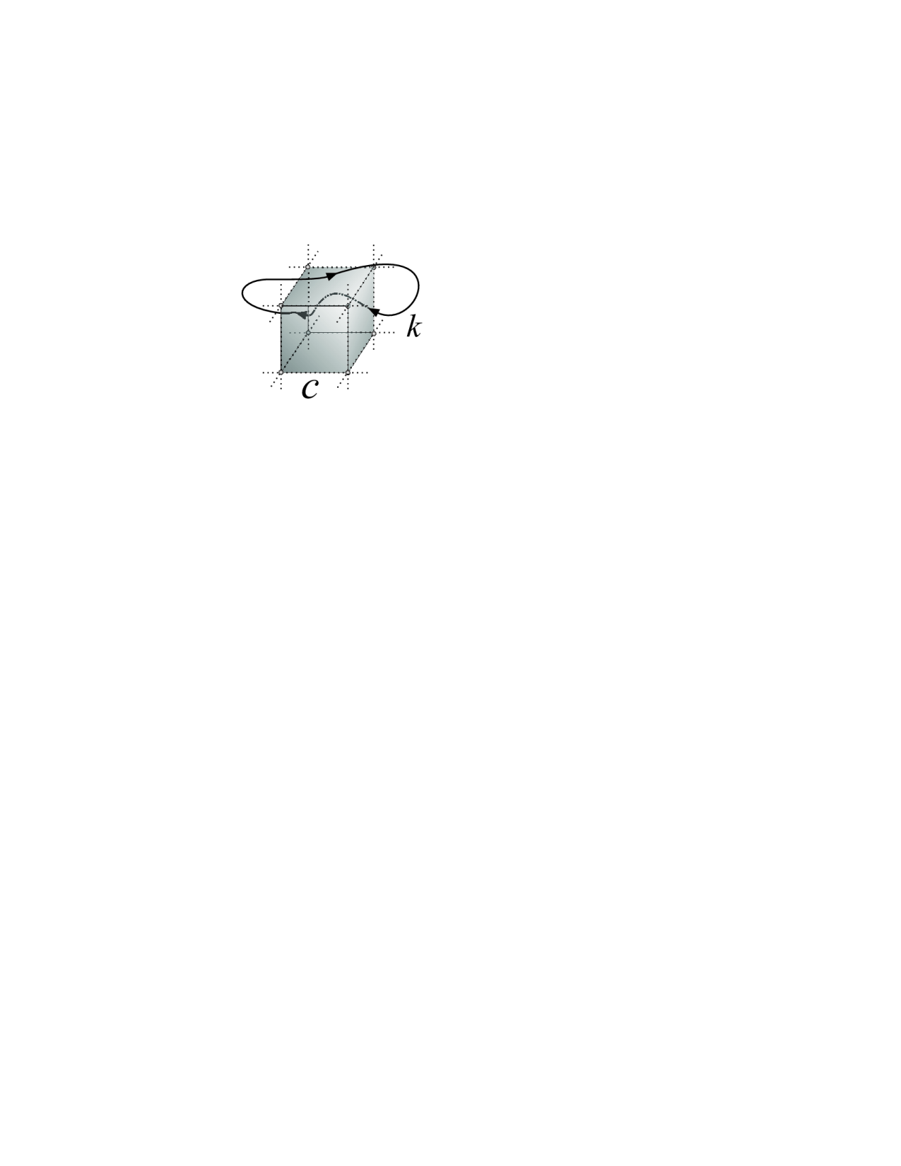
(a)	(b)

Figure 1: Blocking of the continuum monopoles to the lattice in (a) $3D$ and (b) $4D$. In $3D$ the charge corresponding to the lattice cube ${\cal C}$ is given by the total magnetic charge of the continuum monopoles inside this cube. In $4D$ the charge is proportional to the linking number of the monopole trajectory, $k$, with the surface of the three–dimensional cube ${\cal C}$.

Next step is to construct a ”lattice quantity” (for example, the absolute value of the magnetic charge inside a $3D$ cell) and calculate analytically the average of this quantity over all configurations of the continuum monopoles. The value of this averaged quantity would depend on the size of the cell, $b$, and on the parameters of the continuum model ($i.e.$, on $\zeta$ and $g$). Similarly, one can study numerically the same quantity in a purely lattice model ($i.e.$, in the dimensionally reduced quenched SU(2) QCD as in Ref. ref:ishiguro:suzuki:chernodub ), and relate both numerical and analytical results for the density with each other. Since the averaged density depends on the scale $b$, the fitting of the numerical results to the analytically obtained formula gives an information about the parameters of the continuum model, $\zeta$ and $g$. The fitting also provides an information about the self–consistency of this approach, or, in other words, about the validity of the description of the lattice quantities by the continuum model.

Therefore this method allows us to describe the lattice observables by the continuum model. In Ref. ref:ishiguro:suzuki:chernodub the blocking was performed for the monopoles in $3D$ which are the instanton–like objects. Below we generalize this approach to the four dimensional case.

The partition function of the dual superconductor can be described in terms of the monopole trajectories as follows:

$${\cal Z}_{mon}=\int\Sigma{\cal D}k\int{\cal D}B\,\exp\Bigl{\{}-\int{\mathrm{d}}^{4}x\,\Bigl{[}\frac{1}{4g^{2}}F^{2}_{\mu\nu}+ik_{\mu}(x)B_{\mu}(x)\Bigr{]}-S_{int}(k)\Bigr{\}}\,,$$ (1)

where $F_{\mu\nu}=\partial_{\mu}B_{\nu}-\partial_{\nu}B_{\mu}$ is the field stress tensor of the dual gauge field $B_{\mu}$, and $S_{int}(k)$ is the action of the closed monopole currents $k$,

$$k_{\mu}(x)=\oint{\mathrm{d}}\tau\,\frac{\partial{\tilde{x}}_{\mu}(\tau)}{\partial\tau}\,\delta^{(4)}[x-\tilde{x}(\tau)]\,.$$ (2)

Here the $4D$ vector function ${\tilde{x}_{\mu}}(\tau)$ defines the trajectory of the monopole current. In Eq. (1) the integration is carried out over the dual gauge fields and over all possible monopole trajectories (the sum over disconnected parts of the monopole trajectories is also implicitly assumed).

The action in Eq. (1) contains three parts: the kinetic term for the dual gauge field, the interaction of the dual gauge field with the monopole current and the self–interaction of the monopole currents. The integration over the monopole trajectories gives the lagrangian of the dual Abelian Higgs model ref:suzuki:maedan :

$${\cal Z}_{mon}\propto{\cal Z}_{DAHM}=\int{\cal D}\Phi\int{\cal D}B\,\exp\Bigl{\{}-\int{\mathrm{d}}^{4}x\,\Bigl{[}\frac{1}{4g^{2}}F^{2}_{\mu\nu}+\frac{1}{2}|(\partial_{\mu}+iB_{\mu})\Phi|^{2}+V(\Phi)\Bigr{\}}\,,$$ (3)

where $\Phi$ is the complex monopole field. The self–interactions of the monopole trajectories described by the action $S_{int}$ in Eq. (1) lead to the self–interaction of the monopole field $\Phi$ described by the potential term $V(\Phi)$ in Eq. (3).

Now let us embed the hypercubic lattice with the lattice spacing $b$ into the continuum space. The three-dimensional cubes are defined as follows:

$$C_{s,\mu}=\Biggl{\{}b\Bigl{(}s_{\nu}-\frac{1}{2}\Bigr{)}\leq x_{\nu}\leq b\Bigl{(}s_{\nu}+\frac{1}{2}\Bigr{)}\,\,\mbox{for}\,\,\nu\neq\mu\,;\,\,\mbox{and}\,\,x_{\mu}=bs_{\mu}\Biggr{\}}\,,$$ (4)

where $s_{\nu}$ is the dimensionless lattice coordinate of the lattice cube $C_{s,\mu}$ and $x_{\nu}$ is the continuum coordinate. The direction of the $3D$ cube in the $4D$ space is defined by the Lorentz index $\mu$.

As in the three-dimensional example described above, let us consider a configuration of the monopole currents superimposed on the lattice (4). The monopole charge $K_{C}$ inside the lattice cube $C_{s,\mu}$ is equal to the total charge of the continuum monopoles, $k$, which pass through this cube. Geometrically, the total monopole corresponds to the linking number between the cube $C$ and the monopole trajectories, $k$ (an illustration is presented in Fig. 1). The mutual orientation of the cube and the monopole trajectory is obviously important. The corresponding mathematical expression for the monopole charge $K_{C}$ inside the cube $C$ is a generalization of the Gauss linking number to the four dimensional space–time:

$$K_{C}(k)\equiv{I\!\!L}(\partial C,k) = \frac{1}{2}\int\!{\mathrm{d}}^{4}x\int\!{\mathrm{d}}^{4}y\,\epsilon_{\mu\nu\alpha\beta}\,\Sigma^{\partial C}_{\mu\nu}(x)\,k_{\alpha}(y)\,\partial_{\beta}{\cal D}^{(4)}(x-y)$$ (5)

$$= \frac{1}{4\pi^{2}}\int{\mathrm{d}}^{4}x\int{\mathrm{d}}^{4}y\,\epsilon_{\mu\nu\alpha\beta}\,\Sigma^{\partial C}_{\mu\nu}(x)\,k_{\alpha}(y)\,\frac{{(x-y)}_{\beta}}{{|x-y|}^{4}}\,.$$

Here the function $\Sigma^{\partial C}_{\mu\nu}(x)$ is the two–dimensional $\delta$–function representing the boundary $\partial C$ of the cube $C$. In general form it can be written as follows:

$$\Sigma_{\alpha\beta}(x)=\int_{\Sigma}{\mathrm{d}}\tau_{1}{\mathrm{d}}\tau_{2}\,\frac{x_{[\alpha,}(\vec{\tau})}{\partial\tau_{a}}\frac{x_{\beta]}(\vec{\tau})}{\partial\tau_{b}}\,\delta^{(4)}[x-\tilde{x}(\vec{\tau})]\,,$$ (6)

where the four dimensional vector $\tilde{x}(\vec{\tau})$ parameterizes the position of the two–dimensional surface $\Sigma$. The function ${\cal D}^{(4)}$ in Eq. (5) is the inverse Laplacian in four dimensions, $\partial^{2}_{\mu}{\cal D}^{(4)}(x)=\delta^{(4)}(x)$. It is obvious that the lattice currents $K_{s,\mu}$ are closed

$$\partial^{\prime}K=0\,,$$ (7)

due to the conservation of the continuum monopole charge, $\partial_{\mu}k_{\mu}=0$. In Eq. (7) the symbol $\partial^{\prime}$ denotes the backward derivative on the lattice. We present a proof of Eq. (7) in Appendix A.

Let us rewrite the dual superconductor model (3) in terms of the lattice currents $K_{C}$, Eq. (5). To this end we insert the unity,

$$1=\sum\limits_{K_{C}\in Z\!\!\!Z}\,\prod\limits_{C}\delta\Bigl{(}K_{C}-{I\!\!L}(\partial C,k)\Bigr{)}\,,$$ (8)

into the partition function (1) (here $\delta$ represents the Kronecker symbol). Then we integrate the continuum degrees of freedom, $k_{\mu}$ and $B_{\mu}$, getting the partition function in terms of the lattice charges $K_{C}$. The simplest way to do so is to represent the product of the Kronecker symbols in Eq. (8) in terms of the integrals,

$$1=\sum\limits_{K_{C}\in Z\!\!\!Z}\,\Bigl{[}\prod_{C}\int\limits^{\infty}_{-\infty}{\mathrm{d}}\theta_{C}\Bigr{]}\,\exp\Bigl{\{}i\sum_{C}\theta_{C}\,K_{C}-i\int{\mathrm{d}}^{4}x\,k_{\mu}(x){\tilde{B}}_{\mu}(\theta;x)\Bigr{\}}\,,$$ (9)

where

$${\tilde{B}}_{\mu}(\theta;x)=\frac{1}{2}\int\!{\mathrm{d}}^{4}y\,\epsilon_{\mu\nu\alpha\beta}\,\partial_{\nu}{\cal D}^{(4)}(x-y)\,\sum\limits_{C}\theta_{C}\,\Sigma^{\partial C}_{\alpha\beta}(y)\,.$$ (10)

To derive Eqs. (9,10) from Eq. (8) we used relation (5).

Substituting Eq. (9) into Eq. (1) we get:

$${\cal Z}_{mon} = \int\Sigma{\cal D}k\int{\cal D}B\,\sum\limits_{K_{C}\in Z\!\!\!Z}\,\Bigl{[}\prod_{C}\int\limits^{\infty}_{-\infty}{\mathrm{d}}\theta_{C}\Bigr{]}\,\exp\Bigl{\{}i\sum_{C}\theta_{C}\,K_{C}$$ (11)

$$-\int{\mathrm{d}}^{4}\Bigl{[}\frac{1}{4g^{2}}F^{2}_{\mu\nu}+ik_{\mu}(x)\Bigl{(}B_{\mu}(x)+{\tilde{B}}_{\mu}(\theta;x)\Bigr{)}\Bigr{]}-S_{int}(k)\Bigr{\}}\,.$$

One can see that the substitution of the unity (9) effectively shifts the gauge field in the interaction term with the monopole current, $B_{\mu}\to B_{\mu}+{\tilde{B}}_{\mu}$. Therefore the integration over the monopole trajectories, $k_{\mu}$, in Eq. (11) is very similar to the integration which relates Eq. (1) and Eq. (3). Thus, we get:

$${\cal Z}_{mon}\propto{\cal Z}_{DAHM} = \int{\cal D}\Phi\int{\cal D}B\,\sum\limits_{K_{C}\in Z\!\!\!Z}\,\Bigl{[}\prod_{C}\int\limits^{\infty}_{-\infty}{\mathrm{d}}\theta_{C}\Bigr{]}\,\exp\Bigl{\{}i\sum_{C}\theta_{C}\,K_{C}$$ (12)

$$-\int{\mathrm{d}}^{4}x\Bigl{[}\frac{1}{4g^{2}}F^{2}_{\mu\nu}+\frac{1}{2}\Bigl{|}\Bigl{[}\partial_{\mu}+i(B_{\mu}(x)+{\tilde{B}}_{\mu}(\theta;x))\Bigr{]}\Phi\Bigr{|}^{2}+V(\Phi)\Bigr{]}\Bigr{\}}\,.$$

Summarizing this Section, we rewrite the continuum dual superconductor model in terms of the lattice monopole currents, $K$:

$${\cal Z}_{DAHM}=\sum\limits_{K_{x,\mu}\in Z\!\!\!Z}\,e^{-S_{mon}(K)}\,,$$ (13)

where the monopole action is defined via the lattice Fourier transformation:

$$e^{-S_{mon}(K)}=\int\limits^{\infty}_{-\infty}{\cal D}\theta_{C}\,\exp\Bigl{\{}-{\tilde{S}}(\theta)+i(\theta,K)\Bigr{\}}\,,$$ (14)

and the action of the compact lattice fields $\theta$ is expressed in terms of the dual Abelian Higgs model in continuum:

$$e^{-{\tilde{S}}(\theta)}\!=\!\int\!\!{\cal D}\Phi\int\!\!{\cal D}B\,\exp\Bigl{\{}-\!\!\int\!{\mathrm{d}}^{4}x\Bigl{[}\frac{1}{4g^{2}}F^{2}_{\mu\nu}+\frac{1}{2}\Bigl{|}\Bigl{[}\partial_{\mu}+i(B_{\mu}+{\tilde{B}}_{\mu}(\theta)\Bigr{]}\Phi\Bigr{|}^{2}+V(\Phi)\Bigr{]}\Bigr{\}}\,.$$ (15)

Eqs. (10,13,14,15) are the main result of this Section.

III Quadratic part of monopole action

An exact integration over the monopole, $\Phi$, and dual gauge gluon, $B_{\mu}$, fields in Eq. (15) is impossible in a general case. However, in this paper we are interested in the quadratic part of the monopole action which is dominated by the contribution of the one dual gluon exchange. Therefore we do not consider the effect of the fluctuations of the monopole field $\Phi$, which lead to the higher–point interactions in the effective monopole action chernodub . Effectively, the neglect of the quantum fluctuations of the monopole field corresponds to a mean field approximation with respect to this field, $\Phi\to\langle\Phi\rangle$. In this case the AHM action becomes quadratic and Eq. (15) can be rewritten as

$$e^{-{\tilde{S}}(\theta)}\!=\int\!\!{\cal D}B\,\exp\Bigl{\{}-\!\!\int\!{\mathrm{d}}^{4}x\Bigl{[}\frac{1}{4g^{2}}F^{2}_{\mu\nu}+\frac{\eta^{2}}{2}{\Bigl{(}B_{\mu}+{\tilde{B}}_{\mu}(\theta)\Bigr{)}}^{2}\Bigr{]}\Bigr{\}}\,,$$ (16)

where $\eta=|\langle\Phi\rangle|$ is the monopole condensate.

The Gaussian integration over the dual gauge field can be done explicitly. In momentum space the effective action (up to an irrelevant additive constant) reads as follows:

$${\tilde{S}}(\theta)=\frac{\eta^{2}}{2}\int\frac{{\mathrm{d}}^{4}p}{(2\pi)^{4}}\,{\tilde{B}}_{\mu}(\theta,p)\,\frac{p^{2}\delta_{\mu\nu}-p_{\mu}p_{\nu}}{p^{2}+M_{B}^{2}}\,{\tilde{B}}_{\mu}(\theta,-p)\,,$$ (17)

where ${\tilde{B}}_{\mu}(\theta,p)$ is related to the field ${\tilde{B}}_{\mu}(\theta,x)$, given in Eq. (10), by a continuum Fourier transformation:

$${\tilde{B}}_{\mu}(\theta,p)=\frac{b^{3}}{p^{2}}\sum\limits_{s,\alpha}[p^{2}\,\delta_{\mu\alpha}Q_{\alpha}(pb)-p_{\mu}p_{\alpha}\,Q_{\alpha}(pb)]e^{-ib(p,s)}\,\theta_{s,\alpha}\,,$$ (18)

with

$$Q_{\mu}(x)=\prod\limits_{\nu\neq\mu}\frac{\sin x_{\nu}/2}{x_{\nu}/2}\,.$$ (19)

To get Eq. (18) from Eq. (10) we notice that

$$\frac{1}{2}\epsilon_{\mu\nu\alpha\beta}\,\Sigma^{\partial C}_{\alpha\beta}(x)=\partial_{[\mu},V^{C}_{\nu]}(x)\,,$$ (20)

where $V^{C}_{\mu}$ is the characteristic function of the lattice cell $C_{s,\mu}$. Namely, the characteristic function of the $3D$ cube with the lattice coordinate $s_{\mu}$ and the direction $\alpha$ is

$$V_{\mu}(C_{s,\alpha},x)=\delta_{\mu,\alpha}\,\delta(x_{\alpha}-bs_{\alpha})\prod\limits_{\gamma\neq\alpha}\Theta(b(s_{\gamma}+1/2)-x_{\gamma})\cdot\Theta(x_{\gamma}-b(s_{\gamma}-1/2))\,,$$ (21)

where $\Theta(x)$ is the Heaviside function. The Fourier transform of the function (21) is

$$V_{\mu}(C_{x,\alpha},p)=\delta_{\mu,\alpha}\,b^{3}\,Q_{\alpha}(pb)\,e^{-ib(p,s)}\,.$$ (22)

Substituting Eq. (18) into Eq. (17) and changing the momentum variable, $q=bp$, we get the following expression for the quadratic action:

$${\tilde{S}}(\theta)=\frac{\eta^{2}b^{2}}{2}\sum_{s,s^{\prime}}\sum_{\alpha,\alpha^{\prime}}\theta_{s,\alpha}{\cal F}^{-1}_{ss^{\prime},\alpha\alpha^{\prime}}\theta_{s^{\prime}\alpha}\theta_{s^{\prime},\alpha^{\prime}}\,,$$ (23)

where

$${\cal F}^{-1}_{ss^{\prime},\alpha\alpha^{\prime}}=\int\frac{{\mathrm{d}}^{4}q}{(2\pi)^{4}}\frac{q^{2}\delta_{\alpha\alpha^{\prime}}-q_{\alpha}q_{\alpha^{\prime}}}{q^{2}+\mu^{2}}Q_{\alpha}(q)Q_{\alpha^{\prime}}(q)\,e^{iq(s^{\prime}-s)}\,.$$ (24)

Here we have introduced the dimensionless parameter

$$\mu=M_{B}\,b\,.$$ (25)

Next step is to substitute Eq. (23) into Eq. (14) and integrate over the variables $\theta$ to get the quadratic monopole action:

$$S_{\mathrm{mon}}(K)=\sum_{s,s^{\prime}}\sum_{\alpha,\alpha^{\prime}}K_{s,\alpha}\,{\cal S}_{ss^{\prime},\alpha\alpha^{\prime}}\,K_{s^{\prime},\alpha^{\prime}}\,,\quad{\cal S}_{ss^{\prime},\alpha\alpha^{\prime}}=\frac{1}{2\,\eta^{2}b^{2}}{\cal F}_{ss^{\prime},\alpha\alpha^{\prime}}\,.$$ (26)

We could not find an explicit form for the operator ${\cal F}^{-1}$ and therefore we calculate it in the $\mu\to\infty$ limit. This limit corresponds to large values of $b$ which are consistent with the quadratic form of the monopole action chernodub . The details of the calculation are given in Appendix B, and the result is:

$${\cal F}^{-1}_{ss^{\prime},\alpha\alpha^{\prime}}\!\! = \frac{\delta_{\alpha\alpha^{\prime}}}{4\pi}\delta_{s_{\alpha},s_{\alpha}^{\prime}}\Bigl{[}\Gamma(0,t_{UV}\mu^{2})\,{\cal D}^{(3)}_{\alpha}({(\vec{s}-\vec{s}^{\prime})}_{\perp})$$ (27)

$$\qquad\qquad\quad+\frac{2}{\mu}{\cal G}_{\alpha}({(\vec{s}-\vec{s}^{\prime})}_{\perp})+\frac{3}{\pi\mu^{2}}{\cal H}_{\alpha}({(\vec{s}-\vec{s}^{\prime})}_{\perp})\Bigr{]},$$

$${\cal D}^{(3)}_{\alpha}(\vec{s}) = \sum_{\stackrel{{\scriptstyle\mbox{\footnotesize cyclic}}}{{i,j,k\neq\alpha}}}\Delta_{s_{i}}\delta_{s_{j}}\delta_{s_{k}}\,,\quad{\cal G}_{\alpha}(\vec{s})=\sum_{\stackrel{{\scriptstyle\mbox{\footnotesize cyclic}}}{{i,j,k\neq\alpha}}}\Delta_{s_{i}}\Delta_{s_{j}}\delta_{s_{k}}\,,\quad{\cal H}_{\alpha}(\vec{s})=\prod_{i\neq\alpha}\Delta_{s_{i}}\,.$$

Here ${\cal D}^{(3)}_{\alpha}(\vec{s}_{\perp})$ is the three-dimensional Laplacian acting in a timeslice perpendicular to the direction $\hat{\alpha}$, $\delta_{s}$ is the Kronecker symbol, $\Delta_{s}\equiv{\cal D}^{(1)}(s)$ is the one–dimensional Laplacian operator (double derivative) defined in Eq. (75), $\Gamma(a,x)$ is the incomplete gamma function and $t_{UV}$ is an ultraviolet cutoff. In Eq. (27) exponentially suppressed corrections of the order $O(e^{-{\mathrm{const}}\mu})$ are omitted.

Inverting the operator (27) and expanding it in inverse powers of $\mu$ we get the quadratic operator ${\cal S}$ in the monopole action (26):

$${\cal S}_{ss^{\prime},\alpha\alpha^{\prime}} = \frac{2\pi}{\eta^{2}b^{2}\,\Gamma}\cdot\delta_{\alpha\alpha^{\prime}}\delta_{s_{\alpha},s_{\alpha}^{\prime}}\cdot\Bigl{[}{\cal D}^{-1}_{\alpha}-\frac{2}{\mu\Gamma}\,{\cal D}^{-1}_{\alpha}\,{\cal G}_{\alpha}\,{\cal D}^{-1}_{\alpha}$$ (28)

$$+\frac{1}{\pi\mu^{2}\Gamma^{2}}\Bigl{(}4\pi\,{\cal D}^{-1}_{\alpha}\,{\cal G}_{\alpha}\,{\cal D}^{-1}_{\alpha}\,{\cal G}_{\alpha}\,{\cal D}^{-1}_{\alpha}-3\Gamma{\cal D}^{-1}_{\alpha}{\cal H}_{\alpha}\,{\cal D}^{-1}_{\alpha}\Bigr{)}+O(\mu^{-3})\Bigr{]}_{{(\vec{s}-\vec{s}^{\prime})}_{\perp}}\,.$$

where ${\cal D}_{\alpha}\equiv{\cal D}^{(3)}_{\alpha}$, $\Gamma\equiv\Gamma(0,t_{UV}M^{2}_{B}\,b^{2})$. The operator expansion in Eq. (28) is written in a symbolic form.

IV Monopole action in quenched SU(2) QCD

Having determined the action of the blocked monopoles analytically, we are going to the same in the quenched SU(2) QCD using numerical calculations. We simulate the quenched SU(2) gluodynamics with the lattice Wilson action, $S(U)=-\frac{\beta}{2}\sum_{P}{\mathrm{Tr}}U_{P}$, where $\beta$ is the coupling constant and $U_{P}$ is the SU(2) plaquette constructed from the link fields. All our results are obtained in the Maximal Abelian (MA) gauge kronfeld which is defined by the maximization of the lattice functional

$$R=\sum_{s,\hat{\mu}}{\rm Tr}\Big{(}\sigma_{3}\widetilde{U}(s,\mu)\sigma_{3}\widetilde{U}^{\dagger}(s,\mu)\Big{)}\,,$$ (29)

with respect to the SU(2) gauge transformations $U(s,\mu)\to\widetilde{U}(s,\mu)=\Omega(s)U(s,\mu)\Omega^{\dagger}(s+\hat{\mu})$. The local condition of maximization can be written in the continuum limit as the differential equation $(\partial_{\mu}+igA_{\mu}^{3})(A_{\mu}^{1}-iA_{\mu}^{2})=0$. Both this condition and the functional (29) are invariant under residual U(1) gauge transformations, $\Omega^{\mathrm{Abel}}(\omega)={\mathrm{diag}(e^{i\omega(s)},e^{-i\omega(s)})}$.

After the gauge fixing is done we get the Abelian variables applying the Abelian projection to the non–Abelian link variables. The Abelian gauge field is extracted from the $SU(2)$ link variables as follows:

$$\widetilde{U}(s,\mu)=\left(\begin{array}[]{cc}(1-|c(s,\mu)|^{2})^{1/2}&-c^{*}(s,\mu)\\ c(s,\mu)&(1-|c(s,\mu)|^{2})^{1/2}\end{array}\right)\left(\begin{array}[]{cc}u(s,\mu)&0\\ 0&u^{*}(s,\mu)\end{array}\right),$$ (34)

where $u(s,\mu)=\exp(i\theta(s,\mu))$ represents the Abelian link field and $c(s,\mu)$ corresponds to the charged (off–diagonal) matter fields. The Abelian field strength $\theta_{\mu\nu}(s)\in(-4\pi,4\pi)$ is defined on the lattice plaquettes by the Abelian link angle $\theta(s,\mu)\in[-\pi,\pi)$ as follows: $\theta_{\mu\nu}(s)=\theta(s,\mu)+\theta(s+\hat{\mu},\nu)-\theta(s+\hat{\nu},\mu)-\theta(s,\nu)$.

To construct the Abelian monopoles we decompose the field strength $\theta_{\mu\nu}(s)$ into two parts,

$$\theta_{\mu\nu}(s)=\bar{\theta}_{\mu\nu}(s)+2\pi m_{\mu\nu}(s)\,,$$ (35)

where $\bar{\theta}_{\mu\nu}(s)\in[-\pi,\pi)$ is interpreted as the electromagnetic flux through the plaquette and $m_{\mu\nu}(s)$ can be regarded as a number of the Dirac strings piercing the plaquette. The elementary ($i.e.$, defined on the $1^{3}$ lattice cubes) monopole currents are determined by the DeGrand-Toussaintdegrand formula:

$$k_{\mu}(s) = \frac{1}{2}\epsilon_{\mu\nu\rho\sigma}\partial_{\nu}m_{\rho\sigma}(s+\hat{\mu}),$$ (36)

where $\partial$ is the forward lattice derivative. The elementary monopole current is defined on a link of the dual lattice and takes values $0,\pm 1,\pm 2$. Moreover the elementary monopole current satisfies the conservation condition by construction,

$$\partial^{\prime}_{\mu}k_{\mu}(s)=0\,,$$ (37)

where $\partial^{\prime}$ is the backward derivative on the dual lattice.

Besides the elementary monopoles one can also study the so called extended monopoles ivanenko . The extended monopoles are usually used to define the monopole current on a cube of a large size without getting artificial lattice corrections of the order of the lattice spacing, $a$. The $n^{3}$ extended monopole is defined on a sublattice with the lattice spacing $b=na$. The explicit construction of the extended monopoles corresponds to a block spin transformation of the monopole currents with the scale factor $n$,

$$k_{\mu}^{(n)}(s)=\sum_{i,j,l=0}^{n-1}k_{\mu}(ns+(n-1)\hat{\mu}+i\hat{\nu}+j\hat{\rho}+l\hat{\sigma})\,.$$ (38)

The spacing $a$ of the original lattice and, consequently, the artificial lattice corrections (which are of the order of $O(a)$) can be arbitrarily small while the size of the blocked monopole can be fixed in physical units. In our studied we have studied $n=2,3,4,6,8$ blocked monopoles on $48^{4}$ lattice.

Applying consecutively the gauge fixing, the Abelian projection and using formula (38) one can construct the Abelian monopole ensemble for any ensemble of the non–Abelian fields of quenched SU(2) QCD. Then using an inverse Monte-Carlo method one can get the effective monopole action. The details of this procedure can be found in Refs. shiba:condensation ; ref:suzuki:shiba ; chernodub . In our simulations we have used 200 configurations on $48^{4}$ lattice. The Maximal Abelian gauge was fixed with the help of the standard iterative procedure.

In general, the monopole action, $S^{{\mathrm{mon}}}_{{\mathrm{eff}}}$, can be represented as a sum of the $n$–point ($n\geq 2$) operators $S_{i}$, Ref. shiba:condensation ; chernodub :

$$S[k]=\sum_{i}g_{i}S_{i}[k]\,,$$ (39)

where $f_{i}$ are coupling constants. In this paper we adopt only the two–point interactions of the form $S_{i}\sim k_{\mu}(s)k_{\mu^{\prime}}(s^{\prime})$ which works well at large values of $b$. Using the inverse Monte-Carlo method we calculate the monopole action parameterized by 27 couplings $g_{i}$. The maximal distance between the interacting currents in this action is $3$ in units of the blocked lattice spacing $b$. The contributions of higher–distance interactions are very small. The mutual separations and directions of the monopole currents corresponding to the couplings $g_{i}$ are summarized in Table 1. We visualize the first seven most essential coupling constants in the monopole action in Figure 2.

coupling	distance	type	coupling	distance	type
$g_{1}$	(0,0,0,0)	$k_{\mu}(s)$	$g_{15}$	(2,1,1,0)	$k_{\mu}(s+2\hat{\mu}+\hat{\nu}+\hat{\rho})$
$g_{2}$	(1,0,0,0)	$k_{\mu}(s+\hat{\mu})$	$g_{16}$	(1,2,1,0)	$k_{\mu}(s+\hat{\mu}+2\hat{\nu}+\hat{\rho})$
$g_{3}$	(0,1,0,0)	$k_{\mu}(s+\hat{\nu})$	$g_{17}$	(0,2,1,1)	$k_{\mu}(s+2\hat{\nu}+\hat{\rho}+\hat{\sigma})$
$g_{4}$	(1,1,0,0)	$k_{\mu}(s+\hat{\mu}+\hat{\nu})$	$g_{18}$	(2,1,1,1)	$k_{\mu}(s+2\hat{\mu}+\hat{\nu}+\hat{\rho}+\hat{\sigma})$
$g_{5}$	(0,1,1,0)	$k_{\mu}(s+\hat{\nu}+\hat{\rho})$	$g_{19}$	(1,2,1,1)	$k_{\mu}(s+\hat{\mu}+2\hat{\nu}+\hat{\rho}+\hat{\sigma})$
$g_{6}$	(2,0,0,0)	$k_{\mu}(s+2\hat{\mu})$	$g_{20}$	(2,2,0,0)	$k_{\mu}(s+2\hat{\mu}+2\hat{\nu})$
$g_{7}$	(0,2,0,0)	$k_{\mu}(s+2\hat{\nu})$	$g_{21}$	(0,2,2,0)	$k_{\mu}(s+2\hat{\nu}+2\hat{\rho})$
$g_{8}$	(1,1,1,1)	$k_{\mu}(s+\hat{\mu}+\hat{\nu}+\hat{\rho}+\hat{\sigma})$	$g_{22}$	(3,0,0,0)	$k_{\mu}(s+3\hat{\mu})$
$g_{9}$	(1,1,1,0)	$k_{\mu}(s+\hat{\mu}+\hat{\nu}+\hat{\rho})$	$g_{23}$	(0,3,0,0)	$k_{\mu}(s+3\hat{\nu})$
$g_{10}$	(0,1,1,1)	$k_{\mu}(s+\hat{\nu}+\hat{\rho}+\hat{\sigma})$	$g_{24}$	(2,2,1,0)	$k_{\mu}(s+2\hat{\mu}+2\hat{\nu}+\hat{\rho})$
$g_{11}$	(2,1,0,0)	$k_{\mu}(s+2\hat{\mu}+\hat{\nu})$	$g_{25}$	(1,2,2,0)	$k_{\mu}(s+\hat{\mu}+2\hat{\nu}+2\hat{\rho})$
$g_{12}$	(1,2,0,0)	$k_{\mu}(s+\hat{\mu}+2\hat{\nu})$	$g_{26}$	(0,2,2,1)	$k_{\mu}(s+2\hat{\nu}+2\hat{\rho}+\hat{\sigma})$
$g_{13}$	(0,2,1,0)	$k_{\mu}(s+2\hat{\nu}+\hat{\rho})$	$g_{27}$	(2,1,1,0)	$k_{\rho}(s+2\hat{\mu}+2\hat{\nu}+\hat{\rho})$
$g_{14}$	(2,1,0,0)	$k_{\nu}(s+2\hat{\mu}+\hat{\nu})$

Table 1: The quadratic interactions in the monopole action determined numerically.

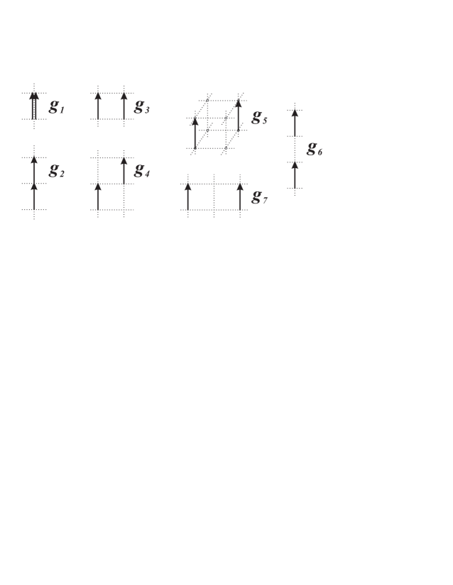
Figure 2: The graphic representation of the first seven types of the quadratic interactions in the lattice monopole action schematized in Table 1.

The action determined above takes into account all monopole trajectories. However, a typical monopole configuration in the confinement phase consists of one large monopole trajectory (percolating cluster) supplemented by a lot of small (ultraviolet) monopole clusters ref:kitahara . The percolating cluster fills the whole volume of the lattice and it makes a dominant contribution to the tension of the chromoelectric string. The properties of the largest percolating cluster were studied both numerically ref:kitahara ; ishiguro:entropy ; ref:boyko and analytically ref:zakharov:clusters . The percolating cluster is associated with the monopole condensate ivanenko:condensate ; shiba:condensation .

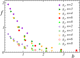
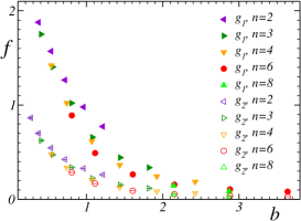
(a)	(b)

Figure 3: The couplings $g_{1}$ and $g_{2}$ of the monopole action (a) for all clusters and (b) for the percolating cluster. In this and other figures the error bars are smaller than the size of symbols and the scale $b$ is shown in units of the string tension.

If our determination of the monopole action is self–consistent then at large scales $b$ the ultraviolet clusters should not give any contribution neither to the monopole action nor to the monopole condensate. The correctness of the first statement for the leading parameter, $g_{1}$, was confirmed in Ref. ishiguro:entropy . In Figures 3(a), (b) we show the couplings $g_{1}$ and $g_{2}$ for all clusters and for the percolating cluster. These couplings show an approximate scaling: they depend only on the product $b=a\cdot n$ and do not depend on the variables $a$ and $n$ separately when $n\geq 3$ are considered. The larger $b$ the better scaling is.

The comparison of the couplings computed on all clusters and on the percolating cluster only are shown in Figures 4(a) and (b). Again, one can clearly observe that at large scales $b$ the coupling constants evaluated on the different types of the monopole ensembles coincide with each other contrary to the small–$b$ case.

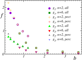
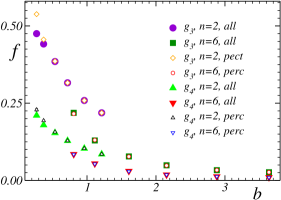
(a)	(b)

Figure 4: The comparison of the couplings (a) $g_{1,2}$ and (b) $g_{3,4}$ computed for all clusters and for the percolating cluster.

V Monopole condensate from monopole action

To get the value of the monopole condensate we have to compare the monopole action calculated analytically in Section III with the numerical results described in Section IV. To this end we first note that due to the closeness of the monopole currents $K_{x,\mu}$ only the transverse part of the monopole operator (28) has a sense. Indeed, the shift of the quadratic operator ${\cal S}\to{\cal S}+\alpha\partial\partial^{\prime}$ (with $\alpha$ being an arbitrary parameter) does not change the monopole action (26) due to conservation condition (7). Therefore, in order to relate the theoretical and numerical results we need to get the transverse part of the operator (28).

A simplest and, on the other hand, a practical way to do extract the transverse part of the quadratic monopole operator is to calculate the monopole action on a set of closed monopole trajectories, $K^{(i)}$. We consider six types of such monopole trajectories which are depicted in Figure 5.

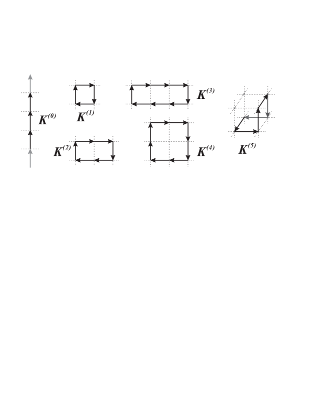
Figure 5: Set of lattice currents used to get transverse elements $f_{i}$ of the monopole action operator.

Let us consider the analytical prediction for the transverse part of the monopole action. Since we are working in the $\mu\gg q$ limit, we disregard $O(\mu^{-1})$ corrections to the quadratic action(28). The validity of such approximation is discussed below. The leading contribution to the monopole action evaluated on closed trajectories $K^{(i)}$ is

$$f_{i}(b)\equiv\frac{S(K^{(i)})}{|K^{(i)}|}=\frac{2\pi\,d_{i}}{\eta^{2}b^{2}\,\Gamma(0,b^{2}M^{2}_{B}t_{UV})}\,,$$ (40)

where $|K^{(i)}|$ is the length of the trajectory $K^{(i)}$ and

$$\begin{array}[]{rclcl}d_{0}&=&{\cal D}^{(3)}(0,0,0)&=&0.248028\dots\,,\\ d_{1}&=&{\cal D}^{(3)}(0,0,0)-{\cal D}^{(3)}(1,0,0)&=&0.166665\dots\,,\\ d_{2}&=&{\cal D}^{(3)}(0,0,0)-\frac{2}{3}{\cal D}^{(3)}(1,0,0)-\frac{1}{3}{\cal D}^{(3)}(2,0,0)&=&0.181055\dots\,,\\ d_{3}&=&{\cal D}^{(3)}(0,0,0)-\frac{3}{4}{\cal D}^{(3)}(1,0,0)-\frac{1}{4}{\cal D}^{(3)}(3,0,0)&=&0.181292\dots\,,\\ d_{4}&=&{\cal D}^{(3)}(0,0,0)-{\cal D}^{(3)}(2,0,0)&=&0.209836\dots\,,\\ d_{5}&=&{\cal D}^{(3)}(0,0,0)-\frac{2}{3}{\cal D}^{(3)}(1,0,0)-\frac{1}{3}{\cal D}^{(3)}(1,1,0)&=&0.176956\dots\,.\end{array}$$ (47)

are the linear combinations of the values of the inverse three-dimensional Laplacian ${\cal D}^{(3)}$ at certain points. The numerical values shown in Eq. (47) correspond to the lattice $48^{3}$. Below we call the combinations $f^{(i)}$ of the couplings as ”transverse couplings”.

Using Table 1 one can get the transverse combinations of couplings corresponding to the numerically calculated action:

$$\begin{array}[]{rclrcl}f_{0}&=&g_{1}+2g_{2}+2g_{6}+2g_{22}\,,&f_{1}&=&g_{1}-g_{3}\,,\\ f_{2}&=&g_{1}+\frac{2}{3}(g_{2}-g_{3}-g_{4})-\frac{1}{3}g_{7}\,,&f_{3}&=&g_{1}+g_{2}-\frac{3}{4}g_{3}-g_{4}+\frac{1}{2}g_{6}-\frac{1}{2}g_{11}-\frac{1}{4}g_{23}\,,\\ f_{4}&=&g_{1}+g_{2}-g_{7}-g_{12}\,,&f_{5}&=&g_{1}-\frac{2}{3}g_{3}-\frac{1}{3}g_{5}\,.\end{array}$$ (51)

Note that the transverse components of the analytical action (40) with two free parameters should describe six transverse combinations (51) obtained numerically. We fit the $f_{i}$ components by (40) independently for each $i=0,1,\dots,5$ and then compare in Table 2 the fitting parameters $\eta$ and $m_{UV}$ as a self–consistency test. Since we are working in the $\mu\gg 1$ limit we fitted the numerical data for the $n=6$ blocked monopoles. A lower value of $n$ corresponds to the smaller scale $b$ and in this case we notice sizable deviations of the numerical results from our fitting function. This is expected because we are working in the limit $b\to\infty$. One the other hand, the higher value, $n=8$, correspond to the small lattice size of the coarse lattice, $(N/n)^{4}=6^{4}$, which may lead to large finite–volume artifacts. Therefore we concentrated on $n=6$ blocked monopoles.

coupling	$\eta/\sqrt{\sigma}$		$\sqrt{t}\,M_{B}/\sqrt{\sigma}$
	all clusters	max cluster	all clusters	max cluster
$f_{0}$	0.521(25)	0.509(23)	0.046(9)	0.042(8)
$f_{1}$	0.577(41)	0.580(45)	0.020(9)	0.022(10)
$f_{2}$	0.565(34)	0.537(37)	0.031(9)	0.025(9)
$f_{3}$	0.544(32)	0.522(35)	0.032(9)	0.026(9)
$f_{4}$	0.554(28)	0.532(30)	0.041(9)	0.034(9)
$f_{5}$	0.591(38)	0.590(42)	0.025(9)	0.026(10)
average	0.552(13)	0.534(13)	0.036(4)	0.031(4)

Table 2: The values of the condensate $\eta$ and the ultraviolet cutoff $t_{UV}$ obtained in a set of independent fits of the $n=6$ transverse monopole couplings (51) by function (40) for the all monopole clusters and for the percolating monopole cluster. The best parameters of the overall fit of $f_{1}\dots f_{6}$ are shown in the last row.

The fits of the transverse couplings of the monopole action corresponding both to all monopole clusters and to the percolating cluster are visualized in Figures 6(a) and (b), respectively.

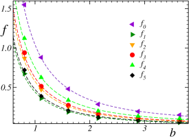
(a)	(b)

Figure 6: The fits of the transverse $n=6$ monopole couplings (51) by function (40) (a) for the all monopole clusters and (b) for the percolating monopole cluster.

The best fit parameters obtained from the fits of different transverse couplings $f_{i}$ (Table 2) are very close to each other what provides a nice self–consistency test of our approach. Moreover, the value of the monopole condensate $\eta$ calculated in large–$b$ limit from the all-clusters and the percolating cluster monopole action are the same within error bars, as expected. The numerical value of the monopole condensate (obtained by averaging of the results of the six independent fits) is $\eta=243(6)$ MeV.

Finally, let us discuss the validity of the large $\mu$ approximation used in this paper. We are working in the range of momenta $b\sqrt{\sigma}\sim 1\dots 4$. The mass of the dual gauge boson obtained from the fitting of the string profile by a classical string solution string:profile is estimated as $M_{B}\approx 1.3~{}\mbox{GeV}\approx 3\sqrt{\sigma}$. Therefore the value of $\mu$, Eq. (25), is in the range $\mu\sim 3\dots 12$. There are two types of corrections to our analytical results: (i) the exponentially suppressed corrections to the operator ${\cal F}^{-1}$ (discussed in Appendix (B)) are smaller than 5%; (ii) the $O(\mu^{-1})$ correction of Eq. (28) is of the order of $10\%$ because of the local nature of the ${\cal G}$ and ${\cal H}$ operators, and due to low values of the inverse Laplacian, ${\cal D}^{(3)}(0,0,0)\approx 1/4$. Thus we estimate the systematic corrections to the value of the monopole condensate to be of the order of $15\%$. Taking into account the systematic errors we get $\eta=243(42)$ MeV.

VI Discussion and Conclusion

We have obtained the value of the monopole condensate using the method of blocking from continuum to the lattice. Namely, we have obtained numerically the effective monopole action in the Maximal Abelian projection of quenched SU(2) lattice QCD. Then we have calculated analytically the effective lattice monopole action starting from the continuum dual Ginzburg–Landau model. In our simulations we restricted ourselves to the large values of the parameter $b$. This parameter defines a scale at which the monopole charge is measured on the lattice. In large–$b$ limit the action of the monopoles is dominated by the quadratic part, and higher monopole interactions are suppressed. Thus in our analytical calculations we have neglected the quantum contributions of the scalar monopole fields which are responsible for the higher order corrections to the effective monopole lagrangian chernodub .

The comparison of the numerical and analytical results for the blocked action gives us the value of the monopole condensate, $\eta=243(42)$ MeV. This value is in a quantitative agreement with another estimation of the monopole condensate, $\eta=194(19)$ MeV, obtained in Ref. string:profile using a completely different method. Moreover, we have shown that our method is self–consistent, since is allows to describe various quadratic interaction of the monopole action using approximately the same values of the monopole condensate.

A few words about the ultraviolet cutoff $t_{UV}$ are now in order. Thus cutoff – which enters the effective monopole action (28) – is an independent fitting parameter of the effective monopole action at large scales, Eq. (40). In this paper we have neglected the fluctuations of the monopole scalar fields since we were working at large scales $b$. Effectively, this corresponds to taking the London limit of the Ginzburg–Landau model. The London limit possesses known logarithmic divergences ($i.e.$, the tension of the Abrikosov vortex is logarithmically divergent function of an ultraviolet scale). The physics of the monopole field fluctuations is ”hidden” in the value of this cutoff. Strictly speaking, we have to renormalize the model and consider the monopole field fluctuations to relate a logarithmic divergence to the values of the physical parameters entering the lagrangian of the model. This procedure becomes meaningful at small scales $b$.

At small values of the scale $b$ the higher order interactions ( four-point, six-point, $etc$) become essential chernodub . Thus at short distances the scalar monopole field contribute to the effective monopole action. From the point of view of the blocking from continuum, at small values of $b$ the couplings of the monopole action become dependent on the parameters of the potential of the monopole field. Thus, a comparison of the effective monopole action with the blocked action at small scales $b$ may allow us to determine the shape of the monopole potential. We discuss this problem in a forthcoming publication in:preparation .

Appendix A Proof of closeness of lattice monopole currents

In order to prove the relation (7) it is convenient to represent the lattice monopole current (5) as the integral over momentum. Using Eq. (20) and Eq. (22) we get:

$$\frac{1}{2}\epsilon_{\mu\nu\alpha\beta}\,\Sigma_{\alpha\beta}(C_{\gamma,s},x)=i(p_{\mu}\,\delta_{\nu\gamma}-p_{\nu}\,\delta_{\mu\gamma})\,b^{3}\,Q_{\gamma}(pb)\,e^{-ib(p,s)}\,,$$ (52)

where $\Sigma_{\alpha\beta}(C,x)\equiv\Sigma^{\partial C}_{\alpha\beta}(x)$, the vector $Q_{\alpha}$ is given in Eq. (19), and no summation over index $\gamma$ is assumed. Then Eq. (5) can be rewritten as follows:

$$K_{s,\gamma} = -b^{3}\int\!\frac{{\mathrm{d}}^{4}p}{(2\pi)^{4}}\,(p_{\mu}\,\delta_{\nu\gamma}-p_{\nu}\,\delta_{\mu\gamma})\,\tilde{k}_{\mu}(-p)\,\frac{p_{\nu}}{p^{2}}\,Q_{\gamma}(pb)\,e^{-ib(p,s)}$$ (53)

$$= -b^{3}\int\!\frac{{\mathrm{d}}^{4}p}{(2\pi)^{4}}\,\tilde{k}_{\gamma}(-p)\,Q_{\gamma}(pb)\,e^{-ib(p,s)}\,,$$

where $\tilde{k}_{\mu}(p)=\int{\mathrm{d}}x\,k_{\mu}(x)\,e^{-i(p,x)}$ is the Fourier transformed continuum monopole current. There is no summation over index $\gamma$ in Eq. (53). To get the second line of Eq. (53) we used the closeness condition of the continuum monopole currents,

$$p_{\mu}\tilde{k}_{\mu}(p)=0\,.$$ (54)

According to Eq. (4) the lattice monopole currents, $K_{s,\mu}$, are associated with the centers of the three–dimensional cubes $C_{s,\mu}$. The positions of the cube centers are characterized by the integer–valued coordinates $s$. The corners of the cubes belong to the original lattice while the monopole currents themselves are associated with the dual lattice. The sites of the dual lattice are shifted by the four–dimensional vector $(1/2,1/2,1/2,1/2)$ with respect to the sites of the original lattice. Thus, the center of the cube $K_{s,\mu}$ does not belong to the dual lattice because the $s_{\mu}$ coordinate of the center of the cube corresponds to the time–slice of the original lattice. In our coordinates, the monopole current defined on the cube $K_{s,\mu}$ must be associated with the point ${}^{*}{s}=s+\hat{\mu}/2$ belonging to the dual lattice.

Thus, the closeness condition (7) at the site ${}^{*}{s}$ of the dual lattice is

$$(\partial^{\prime}K)_{{}^{*}{s}} = \sum^{4}_{\gamma=1}\Bigl{(}K_{{}^{*}{s},\gamma}-K_{{}^{*}{s}-\hat{\gamma},\gamma}\Bigl{)}\equiv\sum^{4}_{\gamma=1}\Bigl{(}K_{s+\frac{1}{2}\hat{\gamma},\gamma}-K_{s-\frac{1}{2}\hat{\gamma},\gamma}\Bigl{)}$$ (55)

$$= 2ib^{3}\int\!\frac{{\mathrm{d}}^{4}p}{(2\pi)^{4}}\,\tilde{k}_{\gamma}(-p)\,\sin(bp_{\gamma}/2)\,Q_{\gamma}(pb)\,e^{-ib(p,s)}\,.$$

Using Eq. (19) we notice that $2\sin(bp_{\gamma}/2)\,Q_{\gamma}(pb)=p_{\gamma}\,Q(pb)$, where the quantity $Q(x)=\prod\nolimits_{\nu}\frac{\sin x_{\nu}/2}{x_{\nu}/2}$ does not carry any Lorentz index. Then Eq. (55) together with the conservation of the continuum monopole charge (54) implies the closeness of the lattice monopole currents,

$$(\partial^{\prime}K)_{s}=ib^{3}\int\!\frac{{\mathrm{d}}^{4}p}{(2\pi)^{4}}\,p_{\gamma}\tilde{k}_{\gamma}(-p)\,\,Q(pb)\,e^{-ib(p,s)}\equiv 0\,.$$

Appendix B Calculation of the operator ${\mathbf{{\cal F}^{-1}}}$

In this Appendix we calculate the expression for the inverse operator ${\cal F}^{-1}$, presented in Eq. (24), for $\mu\equiv M_{B}b\gg 1$.

Let us consider first the diagonal components of the inverse operator ${\cal F}^{-1}$. Without loss of generality we take $\mu=\nu=4$ and $s^{\prime}=0$. We get:

$${\cal F}^{-1}_{s0,44}=\int\frac{{\mathrm{d}}^{4}q}{(2\pi)^{4}}\,\frac{{\vec{q}}^{2}}{q^{2}_{4}+{\vec{q}}^{2}+\mu^{2}}\,\prod^{3}_{i=1}{\Bigl{(}\frac{\sin q_{i}/2}{q_{i}/2}\Bigr{)}}^{2}\cdot e^{iq_{4}s_{4}+i(\vec{q},\vec{s})}\,.$$ (56)

It is convenient to introduce the additional integral,

$$\frac{1}{q^{2}_{4}+{\vec{q}}^{2}+\mu^{2}}=\int^{\infty}_{0}{\mathrm{d}}t\,e^{-(q^{2}_{4}+{\vec{q}}^{2}+\mu^{2})t}\,,$$ (57)

and represent the integral (56) in the form:

$${\cal F}^{-1}_{s0,44}=\int\limits^{\infty}_{0}{\mathrm{d}}t\,e^{-\mu^{2}t}\,P_{0}(s_{4},t)\,\sum_{i=1}^{3}P_{1}(s_{i},t)\prod_{\stackrel{{\scriptstyle j=1}}{{j\neq i}}}^{3}P_{2}(s_{j},t)\,,$$ (58)

where

$$P_{0}(s,t) = \int\limits_{-\infty}^{\infty}\frac{{\mathrm{d}}q}{2\pi}\,e^{-tq^{2}+iqs}=\frac{1}{2\sqrt{\pi t}}\,e^{-s^{2}/4t}\,,$$ (59)

$$P_{1}(s,t) = 4\!\!\int\limits_{-\infty}^{\infty}\!\!\frac{{\mathrm{d}}q}{2\pi}\,\sin^{2}\frac{q}{2}\cdot e^{-tq^{2}+iqs}=-\frac{1}{2\sqrt{\pi t}}\Bigl{(}e^{-(s+1)^{2}/4t}+e^{-(s-1)^{2}/4t}-2e^{-s^{2}/4t}\Bigr{)}\,,$$ (60)

$$P_{2}(s,t) = \int\limits_{-\infty}^{\infty}\frac{{\mathrm{d}}q}{2\pi}\,{\Bigl{(}\frac{\sin q/2}{q/2}\Bigr{)}}^{2}\,e^{-tq^{2}+iqs}=\sqrt{\frac{t}{\pi}}\Bigl{(}e^{-(s+1)^{2}/4t}+e^{-(s-1)^{2}/4t}-2e^{-s^{2}/4t}\Bigr{)}$$ (61)

$$+\frac{1}{2}\Bigl{[}(s+1){\mathrm{Erf}}\Bigl{(}\frac{s+1}{2\sqrt{t}}\Bigr{)}+(s-1){\mathrm{Erf}}\Bigl{(}\frac{s-1}{2\sqrt{t}}\Bigr{)}-2s{\mathrm{Erf}}\Bigl{(}\frac{s}{2\sqrt{t}}\Bigr{)}\Bigr{]}\,,$$

and ${\mathrm{Erf}}(x)$ is the error function,

$${\mathrm{Erf}}(x)=\frac{2}{\sqrt{\pi}}\int^{x}_{0}{\mathrm{d}}y\,e^{-y^{2}}\,.$$

To calculate the off-diagonal components of the inverse operator ${\cal F}^{-1}$ we take $(\mu,\nu)=(1,2)$ and $s^{\prime}=0$ (again, without any loss of generality):

$${\cal F}^{-1}_{s0,12} = \int\frac{{\mathrm{d}}^{4}q}{(2\pi)^{4}}\,\frac{-q_{1}q_{2}}{q^{2}+\mu^{2}}\,\prod^{2}_{i=1}\frac{\sin q_{i}/2}{q_{i}/2}\cdot\prod^{4}_{j=3}{\Bigl{(}\frac{\sin q_{j}/2}{q_{j}/2}\Bigr{)}}^{2}\cdot e^{i(q,s)}$$ (62)

$$= -\int_{0}^{\infty}{\mathrm{d}}t\,e^{-\mu^{2}t}\,\prod^{2}_{i=1}P_{3}(s_{i},t)\cdot\prod^{4}_{j=3}P_{1}(s_{i},t)$$

where

$$P_{3}(s,t) = 2\int\limits_{-\infty}^{\infty}\frac{{\mathrm{d}}q}{2\pi}\,\sin\frac{q}{2}\cdot e^{-tq^{2}+iqs}=\frac{i}{2\sqrt{\pi t}}\Bigl{(}e^{-(2s-1)^{2}/16t}-e^{-(2s+1)^{2}/16t}\Bigr{)}\,.$$ (63)

Eqs.(56-63) represent the exact expressions for the diagonal and off-diagonal elements of the inverse operator ${\cal F}^{-1}$. Unfortunately, due to the presence of the ${\mathrm{Erf}}$–functions in $P_{1}$, Eq. (60), the integrals (56) and (62) can not be taken analytically. However, in the limit $\mu\to\infty$, which corresponds according to Eq. (25) to large blocking scales $b$, leading contributions to these integrals can be easily estimated.

Let us first consider Eq. (56). The main contribution to this integral is coming from the region of small $t$. At small $t$ the error function can be represented as

$${\mathrm{Erf}}(x)=\mathop{\rm sign}(x)-\frac{e^{-x^{2}}}{\sqrt{\pi}x}(1+O(x^{-2}))\quad\mbox{for}\quad x\gg 1\,.$$ (64)

Therefore at general values of $s$ the expression (56) is given by a sum of integrals of the form

$$I(\mu,\tilde{s})=\int_{0}^{\infty}{\mathrm{d}}t\,\exp\{-\mu^{2}t-\tilde{s}^{2}/t+C\,\log t\}\,,$$ (65)

where $C$ is a constant of the order of unity and the quantity $\tilde{s}$ depends on the value of $s$ (i.e., $\tilde{s}=s/2,(s-1)/2$, etc.). The value of $\tilde{s}$ is either of the order of unity or zero. At $\tilde{s}\sim 1$ and large $\mu$ we get $I(\mu,\tilde{s})\sim\exp\{-2\mu\tilde{s}\}\ll 1$. Thus the integral (65) with $\tilde{s}\neq 0$ is exponentially suppressed and therefore it will be neglected below. The leading contribution to the operator ${\cal F}^{-1}$ comes from the integrals of the form (65) with $\tilde{s}=0$ which are saturated at small $t$.

Using the expansion (64) we get in the leading order in the limit $t\to 0$:

$$P_{0}(s,t) = \frac{1}{2\sqrt{\pi t}}\,\delta_{s}+O(e^{-{\mathrm{const}}/t})\,,$$ (66)

$$P_{1}(s,t) = -\frac{1}{2\sqrt{\pi t}}\,\Delta_{s}+O(e^{-{\mathrm{const}}/t})\,,$$ (67)

$$P_{2}(s,t) = \sqrt{\frac{t}{\pi}}\,\Delta_{s}+\delta_{s}+O(e^{-{\mathrm{const}}/t})\,,$$ (68)

$$P_{3}(s,t) = O(e^{-{\mathrm{const}}/t})\,,$$ (69)

where

$$\delta_{s}=\left\{\begin{array}[]{ll}1,&s=0\\ 0,&\mbox{otherwise}\end{array}\right.\,,\qquad\Delta_{s}=\left\{\begin{array}[]{rl}1,&s=1,-1\\ -2,&s=0\\ 0,&\mbox{otherwise}\end{array}\right.\,,$$ (75)

are the Kronecker symbol and the one-dimensional lattice Laplacian, respectively.

According to Eqs. (62,69), the elements with $\mu\neq\nu$ of the operator ${\cal F}^{-1}$ are exponentially suppressed, ${\cal F}^{-1}_{\mu\neq\nu}\sim O(e^{-{\mathrm{const}}\mu})$. As for the diagonal elements of this operator, $\mu=\nu$, we get

$${\cal F}^{-1}_{s0,44} = \frac{1}{4\pi^{2}}\int\limits_{0}^{\infty}{\mathrm{d}}t\,e^{-\mu^{2}t}\,\delta_{s_{4}}\sum_{i=1}^{3}\Delta_{s_{i}}\,\prod_{\stackrel{{\scriptstyle j=1}}{{j\neq i}}}^{3}\Bigl{(}\Delta_{s_{j}}+\sqrt{\frac{\pi}{t}}\delta_{s_{j}}\Bigr{)}+O(e^{-{\mathrm{const}}\mu})$$

$$= \frac{1}{4\pi}\delta_{s_{4}}\,\Bigl{[}\Gamma(0,t_{UV}\mu^{2})\,\Bigl{(}\Delta_{s_{1}}\delta_{s_{2}}\delta_{s_{3}}+\mbox{cyclic}\Bigr{)}+\frac{2}{\mu}\,\Bigl{(}\Delta_{s_{1}}\Delta_{s_{2}}\delta_{s_{3}}+\mbox{cyclic}\Bigr{)}$$

$$+\frac{3}{\pi\mu^{2}}\Delta_{s_{1}}\Delta_{s_{2}}\Delta_{s_{3}}\Bigr{]}+O(e^{-{\mathrm{const}}\mu})\,.$$

Here $\Gamma$ is the incomplete gamma function, $\Gamma(a,x)=\int_{x}^{\infty}t^{a-1}\,e^{-t}\,{\mathrm{d}}t$, and ”cyclic” means cyclic permutations over the indices $s_{i}$. To get Eq. (B) we used Eqs. (58,66,67,68). We also introduced the ultraviolet cutoff, $t_{UV}$, to regularize the logarithmically divergent piece of Eq. (B). Noticing that ${\cal D}^{(3)}_{4}(\vec{s})=\Delta_{s_{1}}\delta_{s_{2}}\delta_{s_{3}}+\mbox{cyclic}$ is the three dimensional Laplacian we get the final expression for ${\cal F}^{-1}$ presented in Eq. (27).

References

- (1) G. ’t Hooft, in High Energy Physics, ed. A. Zichichi, EPS International Conference, Palermo (1975); S. Mandelstam, Phys. Rept. 23, 245 (1976).
- (2) G. ’t Hooft, Nucl. Phys. B190, 455 (1981).
- (3) M. N. Chernodub and M. I. Polikarpov, “Abelian projections and monopoles”, in ”Confinement, duality, and nonperturbative aspects of QCD”, Ed. by P. van Baal, Plenum Press, p. 387, hep-th/9710205; R.W. Haymaker, Phys. Rept. 315, 153 (1999).
- (4) H. Shiba and T. Suzuki, Phys. Lett. B 333, 461 (1994);
- (5) T. Suzuki and I. Yotsuyanagi, Phys. Rev. D42, 4257 (1990); J. D. Stack, S. D. Neiman and R. J. Wensley, Phys. Rev. D 50, 3399 (1994); G. S. Bali, V. Bornyakov, M. Müller-Preussker and K. Schilling, Phys. Rev. D54, 2863 (1996).
- (6) Y. Koma, M. Koma, E. M. Ilgenfritz, T. Suzuki, M. I. Polikarpov, hep-lat/0302006.
- (7) M. N. Chernodub, M. I. Polikarpov, A. I. Veselov, Phys. Lett. B 399, 267 (1997); Nucl. Phys. Proc. Suppl. 49, 307 (1996); A. Di Giacomo and G. Paffuti, Phys. Rev. D 56, 6816 (1997).
- (8) F. V. Gubarev, E. M. Ilgenfritz, M. I. Polikarpov, T. Suzuki, Phys. Lett. B 468, 134 (1999).
- (9) Y. Koma, M. Koma, E.–M. Ilgenfritz, T. Suzuki, hep-lat/0308008.
- (10) S. Maedan and T. Suzuki, Prog. Theor. Phys. 81, 229 (1989); T. Suzuki, Prog. Theor. Phys. 81, 752 (1989).
- (11) V. Singh, D. A. Browne and R. W. Haymaker, Phys. Lett. B 306, 115 (1993); talk of Takayuki Matsuki and R. W. Haymaker at Lattice’03, Tsukuba, Japan, June 2003.
- (12) K. Schilling, G. S. Bali and C. Schlichter, Nucl. Phys. Proc. Suppl. 73, 638 (1999); G. S. Bali, C. Schlichter and K. Schilling, Prog. Theor. Phys. Suppl. 131, 645 (1998).
- (13) M. Baker, J. S. Ball, F. Zachariasen, Phys. Rev. D 37, 1036 (1988), Erratum-ibid. D37, 3785 (1988); ibid. 41, 2612 (1990).
- (14) Y. Matsubara, S. Ejiri, T. Suzuki, Nucl. Phys. Proc. Suppl. 34, 176 (1994); H. Suganuma, S.Sasaki, H.Toki, Nucl. Phys. B435, 207 (1995). M. Baker, N. Brambilla, H. G. Dosch, A. Vairo, Phys. Rev. D 58, 034010 (1998).
- (15) W. Bietenholz and U.J. Wiese, Nucl. Phys. B464, 319 (1996); Phys. Lett. B 378, 222 (1996); W. Bietenholz, Int. J. Mod. Phys. A 15, 3341 (2000).
- (16) M. N. Chernodub, K. Ishiguro and T. Suzuki, hep-lat/0204003; hep-lat/0202020.
- (17) A. S. Kronfeld, M. L. Laursen, G. Schierholz and U. J. Wiese, Phys. Lett. B 198, 516 (1987); A. S. Kronfeld, G. Schierholz and U. J. Wiese, Nucl. Phys. B 293, 461 (1987).
- (18) S.Fujimoto, S.Kato and T.Suzuki, Phys.Lett. B476, 437-447 (2000); M. N. Chernodub, S. Fujimoto, S. Kato, M. Murata, M. I. Polikarpov and T. Suzuki, Phys. Rev. D 62, 094506 M. N. Chernodub, S. Kato, N. Nakamura, M. I. Polikarpov and T. Suzuki, hep-lat/9902013.
- (19) T. A. DeGrand and D. Toussaint, Phys. Rev. D 22, 2478 (1980).
- (20) T. L. Ivanenko, A. V. Pochinsky and M. I. Polikarpov, Phys. Lett. B 252, 631 (1990).
- (21) H. Shiba and T. Suzuki, Phys. Lett. B 351, 519 (1995).
- (22) H. Shiba and T. Suzuki, Phys. Lett. B 343, 315 (1995).
- (23) S. Kitahara, Y. Matsubara, T. Suzuki, Progr. Theor. Phys. 93, 1 (1995).
- (24) M. N. Chernodub, K. Ishiguro, K. Kobayashi and T. Suzuki, hep-lat/0306001.
- (25) P. Y. Boyko, M. I. Polikarpov and V. I. Zakharov, hep-lat/0209075.
- (26) M. N. Chernodub and V. I. Zakharov, Nucl. Phys. B 669, 233 (2003).
- (27) T. L. Ivanenko, A. V. Pochinsky and M. I. Polikarpov, Phys. Lett. B 302, 458 (1993).
- (28) M.N. Chernodub, K. Ishiguro and T.Suzuki, in preparation.