Order from disorder in lattice QCD at high density

Abstract

We investigate the properties of the ground state of strong coupling lattice QCD at finite density. Our starting point is the effective Hamiltonian for color singlet objects, which looks at lowest order as an antiferromagnet, and describes meson physics with a fixed baryon number background. We concentrate on uniform baryon number backgrounds (with the same baryon number on all sites), for which the ground state was extracted in an earlier work, and calculate the dispersion relations of the excitations. Two types of Goldstone boson emerge. The first, antiferromagnetic spin waves, obey a linear dispersion relation. The others, ferromagnetic magnons, have energies that are quadratic in their momentum. These energies emerge only when fluctuations around the large-$N_{c}$ ground state are taken into account, along the lines of “order from disorder” in frustrated magnetic systems. Unlike other spectrum calculations in order from disorder, we employ the Euclidean path integral. For comparison, we also present a Hamiltonian calculation using a generalized Holstein–Primakoff transformation. The latter can only be constructed for a subset of the cases we consider.

I Introduction

The study of quantum chromodynamics at high density is of fundamental importance. In recent years the field has attracted wide attention with renewed interest in color superconductivity (CSC). For a review see Rajagopal:2000wf .

CSC at high density is a prediction of weak-coupling analysis. It is imperative to confirm this prediction by non-perturbative methods. Bringoltz and Svetitsky Bringoltz:2002qc studied high-density quark matter with strong-coupling lattice QCD (see also strong_coupling ). This theory is described by an effective Hamiltonian for color singlet objects. At lowest order in the inverse coupling, the Hamiltonian looks like an antiferromagnet, and describes the dynamics of meson-like objects within a fixed background of baryon number. Higher orders in the inverse coupling add the effective Hamiltonian with kinetic terms for the baryons that are very hard to treat Bringoltz:2002qc . The global symmetry group of the antiferromagnet depends on the formulation of the lattice fermions. For naive, nearest-neighbor fermions, studied here and in Ref. Bringoltz:2002qc, , the symmetry is $U(4N_{f})$. The representation of $U(4N_{f})$ carried by the fields on each site depends on the baryon number on that site.

From the antiferromagnetic effective Hamiltonian one can derive a path integral for a nonlinear sigma model (NLSM). The path integral can be studied in the large-$N_{c}$ limit with semiclassical methods.

Following Ref. Bringoltz:2002qc, , we choose to work with baryon number backgrounds that have the same baryon number $B$ on all sites with $|B|=1,2,\dots,2N_{f}-1$. These backgrounds are close to lattice saturation (that happens for $B=2N_{f}$), but involve relatively simple calculations; The sigma fields on all sites belong to the same manifold and represent the same number of independent fluctuations (see Bringoltz:2002qc ). Any other distribution of baryon number can also be treated with the NLSM, but will involve sigma fields whose structure changes from site to site. This makes the calculations of the semi-classical ground state and excitations less straight forward than presented here and in Ref. Bringoltz:2002qc, . We leave the treatment of non-uniform baryon number backgrounds, together with the kinetic terms for the baryons to future study, as a step towards comparing our results to those of grand canonical approaches.

For the baryon number background we study, the classical ($N_{c}=\infty$) vacuum of the NLSM is hugely degenerate: If one aligns the $\sigma$ fields on the even sites, the field on each odd site can independently wander a submanifold of the original $\sigma$ manifold. It was shown in Bringoltz:2002qc that fluctuations in $O(1/N_{c})$ couple the $\sigma$ fields on the odd sites to each other and give an effective action that lifts the classical degeneracy. The ground state breaks $U(4N_{f})$.

Here we treat the problem in the context of “order from disorder” Aharony ; Ord_disorder ; double_Xchange ; Kagome ; Sachdev ; Henley , a phenomenon known in the study of condensed matter systems. Its essence is that fluctuations of quantum, thermal or even quenched nature can lift a classical degeneracy. A famous example is the Kagomé antiferromagnet Kagome whose classical ground state energy is invariant under correlated rotations of local groups of spins, leading to a degeneracy exponential in the volume. This system has modes with zero energy for all momentum. These zero modes obtain nonzero energy due to quantum fluctuations. The same thing happens in our NLSM. Here we identify the zero modes, show how they get nonzero energy of $O(1/N_{c})$ and calculate their dispersion relations.

We end up with two kinds of Goldstone boson. The first are antiferromagnetic spin waves with a linear dispersion relation. The second kind are ferromagnetic magnons with a quadratic dispersion relation. This is consistent with the loss of Lorentz invariance due to finite density. This set of excitations falls into the pattern described by Chadha and Nielsen Nielsen:hm and by Leutwyler Leutwyler:1993gf in their studies of nonrelativistic field theories. In general, a nonrelativistic system that undergoes spontaneously symmetry breakdown can posses two types of Goldstone boson. The energy of type I bosons is an odd power of their momentum. Their effective field theory has a second time derivative which means that each excitation is described by one real field as in the case of a relativistic scalar field. Type II bosons have a dispersion relation that contains an even power of the momentum. They can appear only in nonrelativistic theories having properties similar to a Schrödinger field theory, namely theories whose action has only a first time derivative. As in the Schrödinger case, each excitation is described by a complex field, or two real fields. The number of Goldstone fields is of course equal to the number $n_{G}$ of broken generators. The counting of massless excitations is summarized by the Chadha–Nielsen counting rule,

$$n_{I}+2n_{II}\geq n_{G},$$ (1)

Where $n_{I}(n_{II})$ are the number of type I and II Goldstone bosons. A well known example is the $SU(2)$ spin system with a collinear ground state , where $n_{G}=2$. The antiferromagnet has two spin waves with a linear dispersion relation ($n_{I}=2,n_{II}=0$) while the ferromagnet has one magnon with a quadratic dispersion relation ($n_{I}=0,n_{II}=1$). As mentioned above in our case both $n_{I}$ and $n_{II}$ are nonzero.

Most discussions of “order from disorder” work in a Hamiltonian (but see Sachdev ; Henley ). We employ instead the Euclidean path integral. In Appendix C we also present a Hamiltonian calculation using a generalized Holstein-Primakoff Randjbar-Daemi:1992zj transformation. The latter can only be constructed for a subset of the cases we consider. The Euclidean calculations are less restrictive in their applicability.

II The Nonlinear Sigma model

In Ref. Bringoltz:2002qc, the problem of lattice QCD at finite densities was transformed to a nonlinear sigma model. In this section we review this approach in order to make the current work self-contained. The starting point is strong coupling QCD with naive fermions. This theory is described by an antiferromagnetic (AF) effective Hamiltonian, which is invariant under a global $U(N)$ symmetry with $N=4N_{f}$. This quantum Hamiltonian is given by

$$H_{\text{eff}}=\frac{J}{2}\sum_{{\bm{n}}\hat{\bm{\mu}}}Q_{\alpha\beta}({\bm{n}})Q_{\beta\alpha}({\bm{n}}+\hat{\bm{\mu}}).$$ (2)

Here $\alpha$ and $\beta$ are Dirac-flavor indices taking values from $1$ to $N$, and $Q_{\alpha\beta}({\bm{n}})$ are the generators of $U(N)$ on site ${\bm{n}}$. The Hilbert space on each site forms an irreducible representation of $U(N)$ which corresponds to a rectangular Young tableau with $N_{c}$ columns. The number $m$ of rows in the Young tableau can vary from site to site and is determined by the local baryon number $B_{\bm{n}}$ according to

$$m_{\bm{n}}=B_{\bm{n}}+N/2.$$ (3)

Therefore, a first step in this Hamiltonian approach is to fix the local baryon number. This restricts the diagonalization of (2) to a certain sector of the Hilbert space, in contrast to other approaches that fix a chemical potential Rajagopal:2000wf ; strong_coupling and let the local baryon number fluctuate. This point makes the comparison between the two approaches nontrivial and out of the scope of this paper. It also reduces the possibility of sketching a phase diagram to identifying the ground state for a given configuration of $B_{\bm{n}}$, as was done in Ref. Bringoltz:2002qc, .

To write the Euclidean path integral we use a generalized spin-coherent-state representation, which turns out to be especially useful in the large-$N_{c}$ limit. The result is a nonlinear sigma model (NLSM), which we proceed to describe.

II.1 Elementary fields

Following Bringoltz:2002qc we study only the case of uniform baryon density, $B_{\bm{n}}=B>0$. The $\sigma$ field at site ${\bm{n}}$ is an $N\times N$ hermitian, unitary matrix that represents the coset space $U(N)/[U(m)\times U(N-m)]$. It can be written as a unitary rotation of the standard matrix $\Lambda$,

$$\sigma_{\bm{n}}=U_{\bm{n}}\Lambda U^{{\dagger}}_{\bm{n}},$$ (4)

with

$$\Lambda=\left(\begin{array}[]{cc}1_{m}&0\\ 0&-1_{N-m}\end{array}\right).$$ (5)

A convenient parameterization Randjbar-Daemi:1992zj for the unitary matrix $U_{\bm{n}}$ is

$$U_{\bm{n}}=\left(\begin{array}[]{ccc}\sqrt{1-\phi_{\bm{n}}\phi^{{\dagger}}_{\bm{n}}}&&\phi_{\bm{n}}\vspace{0.3cm}\\ -\phi^{{\dagger}}_{\bm{n}}&&\sqrt{1-\phi^{{\dagger}}_{\bm{n}}\phi_{\bm{n}}}\end{array}\right).$$ (6)

Here $\phi_{\bm{n}}$ is an $m\times(N-m)$ complex matrix that furnishes coordinates for $U(N)/[U(m)\times U(N-m)]$. Inserting into Eq. (4), we obtain

$$\sigma_{\bm{n}}=\left(\begin{array}[]{ccc}1-2\phi_{\bm{n}}\phi^{{\dagger}}_{\bm{n}}&&-2\phi\sqrt{1-\phi^{{\dagger}}_{\bm{n}}\phi_{\bm{n}}}\vspace{0.3cm}\\ -2\sqrt{1-\phi^{{\dagger}}_{\bm{n}}\phi_{\bm{n}}}\phi^{{\dagger}}_{\bm{n}}&&-1+2\phi^{{\dagger}}_{\bm{n}}\phi_{\bm{n}}\end{array}\right).$$ (7)

Note that $N_{c}$ does not enter the definition of these degrees of freedom.

II.2 The action and the ground state

The action of the NLSM is

$$S=\frac{N_{c}}{2}\int d\tau\left[-\sum_{{\bm{n}}}\text{Tr}\,\Lambda U^{{\dagger}}_{{\bm{n}}}\partial_{\tau}U_{{\bm{n}}}+\frac{J}{2}\sum_{{\bm{n}}\mu}\text{Tr}\,\sigma_{\bm{n}}\sigma_{{\bm{n}}+\hat{\bm{\mu}}}\right].$$ (8)

The overall $N_{c}$ factor allows a systematic treatment in orders of $1/N_{c}$. The classical ground state is found by minimizing the action, which gives field configurations that are $\tau$ independent and minimize the interaction. For $B\neq 0$, this leaves a huge manifold of degenerate field configurations.

To clarify this important point, consider the energy of one link,

$$E=\frac{J}{2}\text{Tr}\,\sigma_{1}\sigma_{2}.$$ (9)

To minimize $E$ we work in a basis where $\sigma_{1}=\Lambda$. The analysis in Bringoltz:2002qc then shows that $\sigma_{2}$ can wander freely in the manifold $U(m)/[U(2m-N)\times U(N-m)]$, a submanifold of $U(N)/[U(m)\times U(N-m)]$. A ground state of the infinite lattice can be constructed replicating $\sigma_{1}$ and $\sigma_{2}$ on the even and odd sites of the lattice. Thus all the $\sigma$ fields on the even sites “point” to $\Lambda$ while on the odd sites, each $\sigma$ field wanders independently in the submanifold. This classical ground state has a huge degeneracy, exponential in the volume. We proceed to analyze its stability.

In Bringoltz:2002qc it was shown that $O(1/N_{c})$ fluctuations lift the degeneracy and choose a collinear ground state, where all the $\sigma$ fields on the odd sites point in the same direction. Without loss of generality the ground state can be chosen to be

$$\sigma_{\text{even}} = \Lambda,$$

$$\sigma_{\text{odd}} = \Lambda_{2}\equiv\left(\begin{array}[]{ccc}1_{2m-N}&0&0\\ 0&-1_{N-m}&0\\ 0&0&1_{N-m}\end{array}\right)=V\Lambda V^{{\dagger}},$$ (13)

with

$$V=\left(\begin{array}[]{ccc}1&0&0\\ 0&0&1\\ 0&-1&0\end{array}\right).$$ (14)

This ground state breaks $U(N)$ to $U(2m-N)\times U(N-m)\times U(N-m)$, with $2(3m-N)(N-m)$ broken generators. This was the main result of Ref. Bringoltz:2002qc, .

III Fluctuations around the ground state

In this section we write an effective action for fluctuations around the ground state up to $O(1/N_{c})$. Working at $O(1)$ first, we identify the zero modes that correspond to the classical degeneracy. We then show how quantum fluctuations give them nonzero energy.

III.1 Effective action and $O(1)$ dispersion relations

The fields $\phi$, suitably shifted, can be identified with the Goldstone bosons around the ground state (13). For the even sites, $\phi=0$ indeed gives $\sigma=\Lambda$. For the odd sites, the vacuum is at

$$\phi=\left(\begin{array}[]{c}0\\ 1_{N-m}\end{array}\right),$$

where the upper part of $\phi$ is a $(2m-N)\times(N-m)$ matrix. We therefore shift $\phi$ on the odd sites according to

$$U^{\prime} \equiv VU,$$

$$\sigma^{\prime}(\phi) \equiv V\sigma(\phi)V^{{\dagger}}.$$ (15)

This gives $\sigma^{\prime}(0)=\Lambda_{2}$. We drop the primes henceforth.

For later convenience we write $\phi$ as

$$\phi=\left(\begin{array}[]{c}\chi\\ \pi\end{array}\right).$$ (16)

Here $\pi$ is an $(N-m)-$ dimensional square matrix while $\chi$ has $(2m-N)$ rows and $(N-m)$ columns. Both are complex. Thus

$$\sigma_{\text{even}}=\left(\begin{array}[]{ccc}1-2\chi\chi^{{\dagger}}&-2\chi\pi^{{\dagger}}&-2\chi\sqrt{1-\phi^{{\dagger}}\phi}\vspace{0.3cm}\\ -2\pi\chi^{{\dagger}}&1-2\pi\pi^{{\dagger}}&-2\pi\sqrt{1-\phi^{{\dagger}}\phi}\vspace{0.3cm}\\ -2\sqrt{1-\phi^{{\dagger}}\phi}\chi^{{\dagger}}&-2\sqrt{1-\phi^{{\dagger}}\phi}\pi^{{\dagger}}&-1+2\phi^{{\dagger}}\phi\\ \end{array}\right),$$ (17)

and

$$\sigma_{\text{odd}}=\left(\begin{array}[]{ccc}1-2\chi\chi^{{\dagger}}&-2\chi\sqrt{1-\phi^{{\dagger}}\phi}&2\chi\pi^{{\dagger}}\vspace{0.3cm}\\ -2\sqrt{1-\phi^{{\dagger}}\phi}\chi^{{\dagger}}&-1+2\phi^{{\dagger}}\phi&2\sqrt{1-\phi^{{\dagger}}\phi}\pi^{{\dagger}}\vspace{0.3cm}\\ 2\pi\chi^{{\dagger}}&2\pi\sqrt{1-\phi^{{\dagger}}\phi}&1-2\pi\pi^{{\dagger}}\\ \end{array}\right).$$ (18)

Each submatrix in Eqs. (17)–(18) has dimensions as indicated in (5).

After scaling $\phi\rightarrow\phi/\sqrt{N_{c}}$ the action takes the form,

$$S = \text{Tr}\,\int d\tau\sum_{\bm{n}}\left[\chi^{{\dagger}}_{\bm{n}}\partial_{\tau}\chi_{\bm{n}}+\pi^{{\dagger}}_{\bm{n}}\partial_{\tau}\pi_{\bm{n}}\right]$$

$$\qquad+J\sum_{{\bm{n}}\hat{\bm{\mu}}}\left[\pi_{\bm{n}}\pi^{{\dagger}}_{\bm{n}}+\pi_{{\bm{n}}+\hat{\bm{\mu}}}\pi^{{\dagger}}_{{\bm{n}}+\hat{\bm{\mu}}}-\pi_{\bm{n}}\pi_{{\bm{n}}+\hat{\bm{\mu}}}-\pi^{{\dagger}}_{\bm{n}}\pi^{{\dagger}}_{{\bm{n}}+\hat{\bm{\mu}}}\right]$$

$$\qquad+\frac{J}{\sqrt{N_{c}}}\sum_{{\bm{n}}\hat{\bm{\mu}}}\left[\chi^{{\dagger}}_{\bm{n}}\chi_{{\bm{n}}+\hat{\bm{\mu}}}\pi_{\bm{n}}-\chi^{{\dagger}}_{{\bm{n}}+\hat{\bm{\mu}}}\chi_{\bm{n}}\pi_{{\bm{n}}+\hat{\bm{\mu}}}+h.c.\right]$$

$$\qquad+\frac{J}{N_{c}}\sum_{{\bm{n}}\hat{\bm{\mu}}}\left[\chi_{\bm{n}}\chi^{{\dagger}}_{\bm{n}}\chi_{{\bm{n}}+\hat{\bm{\mu}}}\chi^{{\dagger}}_{{\bm{n}}+\hat{\bm{\mu}}}-\pi_{\bm{n}}\pi_{{\bm{n}}+\hat{\bm{\mu}}}^{{\dagger}}\pi_{{\bm{n}}+\hat{\bm{\mu}}}^{{\dagger}}\pi_{{\bm{n}}+\hat{\bm{\mu}}}-\pi_{{\bm{n}}+\hat{\bm{\mu}}}\pi_{{\bm{n}}+\hat{\bm{\mu}}}^{{\dagger}}\pi_{\bm{n}}^{{\dagger}}\pi_{\bm{n}}\right.$$

$$\qquad\qquad\qquad-\pi_{\bm{n}}\pi_{\bm{n}}^{{\dagger}}\chi^{{\dagger}}_{{\bm{n}}+\hat{\bm{\mu}}}\chi_{{\bm{n}}+\hat{\bm{\mu}}}-\pi_{{\bm{n}}+\hat{\bm{\mu}}}\pi_{{\bm{n}}+\hat{\bm{\mu}}}^{{\dagger}}\chi^{{\dagger}}_{\bm{n}}\chi_{\bm{n}}$$

$$\qquad\qquad\qquad+\frac{1}{2}\left(\pi_{{\bm{n}}+\hat{\bm{\mu}}}\pi_{{\bm{n}}+\hat{\bm{\mu}}}^{{\dagger}}\pi_{{\bm{n}}+\hat{\bm{\mu}}}\pi_{\bm{n}}+\pi_{{\bm{n}}+\hat{\bm{\mu}}}\pi_{\bm{n}}\pi_{\bm{n}}^{{\dagger}}\pi_{\bm{n}}\right.$$

$$\qquad\qquad\qquad\qquad\left.\left.+\pi_{{\bm{n}}+\hat{\bm{\mu}}}\chi_{{\bm{n}}+\hat{\bm{\mu}}}^{{\dagger}}\chi_{{\bm{n}}+\hat{\bm{\mu}}}\pi_{\bm{n}}+\pi_{{\bm{n}}+\hat{\bm{\mu}}}\pi_{\bm{n}}\chi^{{\dagger}}_{\bm{n}}\chi_{\bm{n}}+h.c.\right)\right]$$

$$\qquad+O(1/N_{c}^{3/2}).$$

The AF structure of the action demands the introduction of an fcc lattice. We write the fields $\phi_{\bm{n}}\equiv\phi^{A}_{\bm{N}}$ with $A=(\text{even},\text{odd})$ and ${\bm{N}}$ belonging to an fcc lattice. We Fourier transform according to

$$\phi^{A}_{\bm{N}}(\tau)=\sqrt{\frac{2}{N_{s}}}\sqrt{\frac{1}{\beta}}\sum_{{\bm{k}},\omega}\phi^{A}_{k}e^{i({\bm{k}}\cdot{\bm{N}}-\omega\tau)}\times\left\{\begin{array}[]{ll}1&A=\text{even}\\ e^{-ik_{z}/2}&A=\text{odd}\end{array}\right..$$ (20)

Here $k\equiv({\bm{k}},\omega)$. In momentum space the action is given by $S=S_{2}+S_{3}+S_{4}$ with (discarding Umklapp terms)

$$S_{2} = \text{Tr}\,\sum_{k}\left(\begin{array}[]{cc}\pi_{k}^{{\text{e}}{\dagger}}&\pi_{-k}^{\text{o}}\end{array}\right)\left(\begin{array}[]{cc}-i\omega+2dJ&-2Jd\gamma_{\bm{k}}\\ -2Jd\gamma_{\bm{k}}&i\omega+2Jd\end{array}\right)\left(\begin{array}[]{c}\pi_{k}^{\text{e}}\\ \pi_{-k}^{{\text{o}}{\dagger}}\end{array}\right)$$ (32)

$$\qquad\quad+\left(\begin{array}[]{cc}\chi_{k}^{{\text{e}}{\dagger}}&\chi_{-k}^{\text{o}}\end{array}\right)\left(\begin{array}[]{cc}-i\omega&0\\ 0&i\omega\end{array}\right)\left(\begin{array}[]{c}\chi_{k}^{\text{e}}\\ \chi_{-k}^{{\text{o}}{\dagger}}\end{array}\right),$$

$$S_{3} = 2Jd\sqrt{\frac{2}{N_{s}N_{c}\beta}}\text{Tr}\,\sum_{kp}\left(\chi_{p}^{{\text{o}}{\dagger}}\chi_{k}^{\text{e}}\pi_{p-k}^{\text{o}}\gamma_{\bm{k}}-\chi_{k}^{{\text{e}}{\dagger}}\chi_{k-p}^{\text{o}}\pi_{p}^{\text{e}}\gamma_{{\bm{k}}-{\bm{p}}}+h.c.\right),$$ (33)

$$S_{4} = 2Jd\frac{2}{N_{s}N_{c}\beta}\text{Tr}\,\sum_{kpq}\left(\chi_{k}^{\text{e}}\chi_{p}^{{\text{e}}{\dagger}}\chi_{q}^{\text{o}}\chi_{q+k-p}^{{\text{o}}{\dagger}}-\pi_{k}^{\text{e}}\pi_{p}^{{\text{e}}{\dagger}}\pi_{q}^{{\text{o}}{\dagger}}\pi^{\text{o}}_{q-k+p}-\pi_{k}^{{\text{e}}{\dagger}}\pi_{p}^{\text{e}}\pi_{q}^{\text{o}}\pi^{{\text{o}}{\dagger}}_{q-k+p}\right.$$

$$\qquad\qquad\qquad\qquad\left.-\chi_{k}^{{\text{e}}{\dagger}}\chi_{p}^{\text{e}}\pi_{q}^{\text{o}}\pi_{q+k-p}^{{\text{o}}{\dagger}}-\pi_{k}^{\text{e}}\pi_{p}^{{\text{e}}{\dagger}}\chi_{q}^{{\text{o}}{\dagger}}\chi_{q-k+p}^{\text{o}}\right)\gamma_{{\bm{k}}-{\bm{p}}}$$

$$\qquad\qquad\qquad\qquad+\frac{1}{2}\left(\left(\pi_{k}^{{\text{e}}{\dagger}}\pi_{p}^{\text{e}}+\chi_{k}^{{\text{e}}{\dagger}}\chi_{p}^{\text{e}}\right)\left(\pi^{\text{o}}_{k-p-q}\pi_{q}^{\text{e}}+\pi_{-q}^{{\text{e}}{\dagger}}\pi_{-(k-p-q)}^{{\text{o}}{\dagger}}\right)\right.$$

$$\qquad\qquad\qquad\qquad\qquad\left.\left(\pi_{k}^{{\text{o}}{\dagger}}\pi_{p}^{\text{o}}+\chi_{k}^{{\text{o}}{\dagger}}\chi_{p}^{\text{o}}\right)\left(\pi^{\text{e}}_{k-p-q}\pi_{q}^{\text{o}}+\pi_{-q}^{{\text{o}}{\dagger}}\pi_{-(k-p-q)}^{{\text{e}}{\dagger}}\right)\right)\gamma_{{\bm{k}}-{\bm{p}}-{\bm{q}}}.$$

$\gamma_{\bm{k}}$ is given by

$$\gamma_{{\bm{k}}}=\frac{1}{d}\sum_{\mu=1}^{d}\cos{k_{\mu}/2}.$$ (35)

At large $N_{c}$, $S_{3}$ and $S_{4}$ are small perturbations. The bare propagators can be read from $S_{2}$,

$$\left(G^{\pi}_{k}\right)_{AB} = \frac{1}{\omega^{2}+4J^{2}d^{2}E^{2}_{\bm{k}}}\left(\begin{array}[]{cc}i\omega+2Jd&2Jd\gamma_{\bm{k}}\\ 2Jd\gamma_{\bm{k}}&-i\omega+2Jd\end{array}\right)_{AB},$$ (38)

$$\left(G^{\chi}_{k}\right)_{AB} = \left(\begin{array}[]{cc}-1/i\omega&0\\ 0&1/i\omega\end{array}\right)_{AB}.$$ (41)

(The propagators are diagonal in the internal group indices.) Here $E_{\bm{k}}=\sqrt{1-\gamma_{\bm{k}}^{2}}$. The poles of the propagators give the dispersion relations of the various bosons at $O(1)$. The result is

$$\omega^{2}+(2JdE_{\bm{k}})^{2}=0\qquad\qquad\text{for $\pi$},$$ (42)

and

$$\omega=0\qquad\qquad\qquad\qquad\qquad\text{for $\chi$}.$$ (43)

The $\pi$ excitations are $2(N-m)^{2}$ AF spin waves. At $B=0$ they are the only excitations. It is easy to verify that the Euclidean dispersion relation is $\omega^{2}\sim-|{\bm{k}}|^{2}$ at low momentum. The $\chi$ excitations are $4(N-m)(2m-N)$ zero modes (“soft” modes). Their energy is zero for all momentum, a sign of the local degeneracy of the classical ground state discussed above.

We conclude this subsection by classifying the different excitations according to their $U(2m-N)\times U(N-m)\times U(N-m)$ representations. We denote a representation by

$$(r_{1},r_{2},r_{3})^{(q_{1},q_{2},q_{3})}.$$ (44)

Here $r_{1}$ denotes the representation of $SU(2m-N)$, and $r_{2,3}$ denote the representations of the two $SU(N-m)$ subgroups. $q_{i}$ are the charges of the excitations under the remaining $U(1)$ factors of the unbroken subgroup. These are generated by the following diagonal matrices.

$$1_{N},\qquad\left(\begin{array}[]{ccc}1_{2m-N}&0&0\\ 0&0&0\\ 0&0&0\end{array}\right),\quad\text{and}\quad\left(\begin{array}[]{ccc}0&0&0\\ 0&1_{N-m}&0\\ 0&0&-1_{N-m}\end{array}\right).$$ (45)

We give the different representations in Table 1. The crucial point is that the AF spin waves and the zero modes reside is completely different representations. This means that the separation between these excitations in the $O(1)$ spectrum will survive at higher orders and that mixing can not occur.

Field	Representation	Dimension
$\pi$	$\left(1,N-m,\overline{N-m}\right)^{(0,0,+2)}$	$(N-m)^{2}$
$\chi_{\text{even}}$	$\left(2m-N,1,\overline{N-m}\right)^{(0,+1,+1)}$	$(2m-N)(N-m)$
$\chi_{\text{odd}}$	$\left(2m-N,\overline{N-m},1\right)^{(0,+1,-1)}$	$(2m-N)(N-m)$

Table 1: $U(2m-N)\times U(N-m)\times U(N-m)$ representations of the excitations. The conjugate fields belong to the conjugate representations. $n(\overline{n})$ stands for the fundamental(its conjugate) representation of $SU(n)$ and $1$ stands for a singlet.

III.2 Self energy calculation and $O(1/N_{c})$ dispersion relations of the $\chi$ fields

In this section we calculate the self energy of the $\chi$ fields to first order in $1/N_{c}$. We shall see that the poles in the soft modes propagators move away from zero energy in this order. The Feynman rules for this problem are presented in Appendix A. We treat $S_{3}$ and $S_{4}$ as perturbations to $S_{2}$ and present the contributions to the self energy in Fig. 1.

Figure 1: Dyson equation for the self energy of the $\chi$ fields. Solid lines correspond to the $\pi$ propagators and dashed lines to the $\chi$ propagators.

Since the $\chi$ propagator is divergent at $\omega=0$ for all ${\bm{k}}$, one must insert its self energy self-consistently, making the replacement

$$\left(G^{\chi}_{k}\right)^{-1}\rightarrow\left(G^{\chi}_{k}\right)^{-1}-\Sigma_{k}.$$

$\Sigma$ is a matrix coupling odd and even degrees of freedom according to

$$\Sigma=\left(\begin{array}[]{cc}\Sigma_{1}&\Sigma_{2}\\ \Sigma_{2}^{*}&\Sigma_{1}^{*}\end{array}\right).$$ (46)

Thus the $\chi$ propagator is replaced by

$$G^{\chi}_{k}=\frac{1}{(-i\omega-\Sigma_{1,k})(i\omega-\Sigma_{1,k}^{*})-|\Sigma_{2,k}|^{2}}\left(\begin{array}[]{cc}i\omega-\Sigma_{1,k}^{*}&\Sigma_{2,k}\\ \Sigma_{2,k}^{*}&-i\omega-\Sigma_{1,k}\end{array}\right).$$ (47)

Here we assume that both matrices $\Sigma_{1,k}$ and $\Sigma_{2,k}$ are diagonal in group space and that

$$\text{Re}\,\Sigma_{1,k}<0$$ (48)

for the stability of the path integral.

In Appendix B we derive self-consistent equations for $\Sigma_{1,k}$ and $\Sigma_{2,k}$. Defining $\tanh{\theta_{\bm{k}}}=-\text{Re}\,\Sigma_{2,(0,{\bm{k}})}/\text{Re}\,\Sigma_{1,(0,{\bm{k}})}$, we write these equations in the form of a single integral equation,

$$(N-m)\tanh{\theta_{\bm{k}}}=\frac{{\displaystyle\int_{\text{BZ}}\left(\frac{dq}{4\pi}\right)^{d}I_{2}({\bm{q}},{\bm{k}})\sinh{\theta_{\bm{q}}}}}{{\displaystyle\int_{\text{BZ}}\left(\frac{dq}{4\pi}\right)^{d}I_{1}({\bm{q}},{\bm{k}})\cosh{\theta_{\bm{q}}}-\eta({\bm{k}})}}\equiv\frac{\beta_{\bm{k}}}{\alpha_{\bm{k}}}.$$ (49)

$\eta({\bm{k}})$ and $I_{1,2}({\bm{q}},{\bm{k}})$ are defined in Appendix B. The poles of the propagators may then be obtained from (47) [see Eq. (66)]. The dispersion relations turn out to be

$$\pm i\omega = \frac{2Jd}{N_{c}}\sqrt{(N-m)^{2}\alpha^{2}_{\bm{k}}-\beta^{2}_{\bm{k}}}$$

$$= \frac{2Jd(N-m)}{N_{c}}\alpha_{\bm{k}}\sqrt{1-\tanh^{2}{\theta_{\bm{k}}}}$$

$$\equiv \frac{2Jd(N-m)}{N_{c}}\epsilon_{\bm{k}}.$$

The solution of Eq. (49) for $d=3$ can be obtained numerically by assuming that the function $\theta_{\bm{k}}$ depends only on $|{\bm{k}}|$ in most of the Brillouin zone. We plot the solution in Fig. 2 for $N-m=1,2,3,4,5$. Recall that the baryon density is given by $B=m-N/2$. Thus for $N_{f}\leq 3$ we cover all baryon density short of saturation.

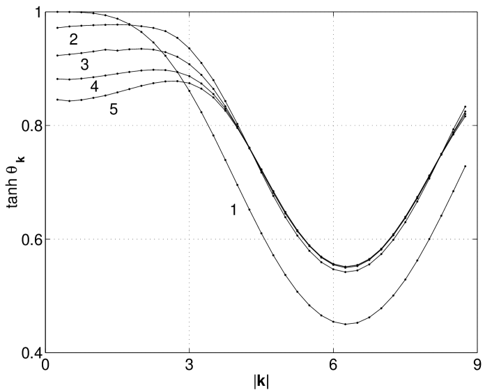
Figure 2: Solution of Eq. (49) for $N-m=1,2,3,4,5$.

The form of $\epsilon_{\bm{k}}$ is shown in Fig. 3. It is easy to check that the bosons are massless, since $\eta(0)=I_{1,2}({\bm{q}},0)=0$ implies that $\alpha_{{\bm{k}}}$ and $\beta_{{\bm{k}}}$ vanish at ${\bm{k}}=0$. This is of course a direct result of the Ward identities concerning the global $U(N)$ symmetry. Moreover, near ${\bm{k}}=0$ both $\alpha$ and $\beta$ have a quadratic dependence on $|{\bm{k}}|$. This means that at low momenta $\epsilon_{\bm{k}}\sim|{\bm{k}}|^{2}$, characteristic of ferromagnetic magnons. A possible exception is the case $N-m=1$. There we see that at low momenta, $\tanh{\theta_{\bm{k}}}\rightarrow 1$ and thus it is possible that $\epsilon_{\bm{k}}\sim|{\bm{k}}|^{2+p}$ with $p$ a positive integer.

Finally we recall that the relation between the number of $\chi$ fields and the number of physical excitations depends on the dispersion relation. Because the soft modes obey $\epsilon_{\bm{k}}\sim|{\bm{k}}|^{2}$, the $4(N-m)(2m-N)$ fields describe only half that many ferromagnetic magnons. The case of $N-m=1$ might be different depending on whether $p$ is odd or even.

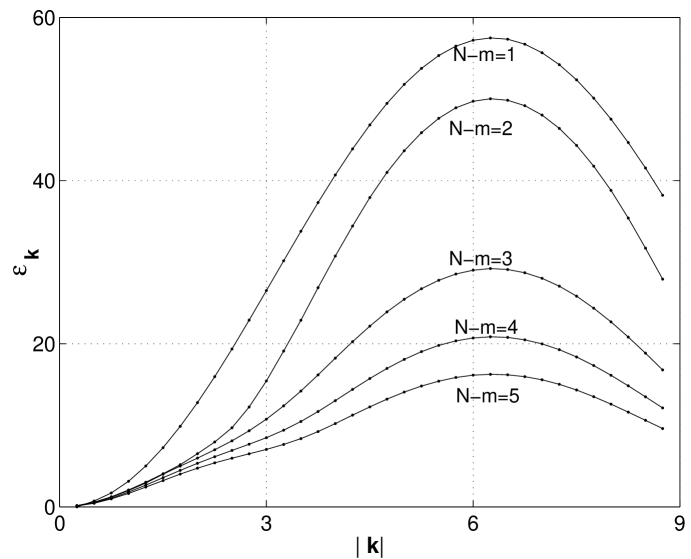
Figure 3: Rescaled energy of the $\chi$ bosons for for $N-m=1,2,3,4,5$. The energy for $N-m=1$ is divided by a factor of $7$ in order to present it on the same scale with the other cases.

IV Summary and discussion

We find two kinds of low energy excitations corresponding to type I and type II Goldstone bosons Nielsen:hm ; Leutwyler:1993gf . The type I bosons are $2(2N_{f}-B)^{2}$ antiferromagnetic spin waves that have a linear dispersion relation. Including quantum fluctuations of $O(1/N_{c})$ we also have $4B(2N_{f}-B)$ type II bosons. We call them ferromagnetic magnons since they derive their energy from the effective ferromagnetic interaction Bringoltz:2002qc between next-nearest-neighbor sites, produced at $O(1/N_{c})$. As typical for magnons, their dispersion relation is quadratic is momentum.

The mechanism that removed the classical degeneracy and gave energy to the type II Goldstone bosons is known in the condensed matter literature as order from disorder Aharony ; Ord_disorder ; double_Xchange ; Kagome ; Sachdev ; Henley . It takes place in systems that posses a classical degenerate ground state. For example we mention the double exchange model double_Xchange and the Kagomé antiferromagnet Kagome . There, the classical ground state energy is invariant under a rotation of local groups of spins making it exponentially degenerate, like in our problem. It is worth recalling that the zero density system is also classically degenerate Bringoltz:2002qc ; Smit:1980nf . There, one can realize the baryon distribution by putting baryon numbers $B$ and $-B$ on the even and odd sites. At $O(1)$, the ground state energy does not depend on $B$. This leads to a discretely degenerate ground state. At $O(1/N_{c})$, order from disorder occurs and quantum fluctuation remove this degeneracy to pick out a ground state with $B=0$.

The energy scale of the type II Goldstone bosons is smaller by a factor of $N_{c}$ compared to that of the type I bosons. This points to a possible hierarchy of phase transitions at finite temperature which can be described by a classical model that has the Hamiltonian

$$H=J_{1}\hskip 2.84544pt\text{Tr}\,\sum_{{\bm{n}}\hat{\bm{\mu}}}\left[\sigma_{\bm{n}}\sigma_{{\bm{n}}+\hat{\bm{\mu}}}\right]-J_{2}\hskip 2.84544pt\text{Tr}\,\sum_{{\bm{n}}\hat{\bm{\mu}}}\left[\sigma_{\bm{n}}\sigma_{{\bm{n}}+2\hat{\bm{\mu}}}\right].$$ (51)

For $J_{2}=0$, the ground state will be highly degenerate as above. A small positive value of $J_{2}$ removes this degeneracy and picks out a ferromagnetic alignment of the next-nearest-neighbor $\sigma$ fields. Thus for $T\ll J_{1,2}$ the ground state is invariant only under

$$U(N-m)\times U(N-m)\times U(2m-N).$$ (52)

This symmetry pattern will persists until some finite temperature $T_{c}^{\text{FM}}\sim J_{2}$. For $T>T_{c}^{\text{FM}}$ the ferromagnetic magnons melt the magnetization and restore some of the symmetry. This situation will persists until a second temperature $T_{c}^{\text{AFM}}\sim J_{1}$ where the symmetry will be restored completely. As long as $J_{1}\gg J_{2}$ (which corresponds to $N_{c}\gg 1$ in our system), the hierarchy of phase transitions is well defined.

Finally we mention that recent works Continuum_mu on effective field theories for dense QCD also predict the existence of type II Goldstone bosons. It is tempting to identify these with our ferromagnetic magnons. First, however, one must reduce the artificial $U(4N_{f})$ symmetry of the action to the physical chiral symmetry. We defer this important issue to further publications.

Appendix A Feynman rules

The following are the Feynman rules extracted from Eqs. (32)–(III.1). $A=({\text{e}},{\text{o}})$ stands for even and odd respectively. Latin indices take values in the range $[1,(N-m)^{2}]$ while Greek indices take values in the range $[1,(N-m)(2m-N)]$. The propagators are given in Fig. 4. The vertices extracted from the cubic and quartic interactions [Eqs. (33)–(III.1)] are given in Figs. 5– 6.

Figure 4: Propagators.

Figure 5: Vertices corresponding to the cubic interaction.

Figure 6: Vertices corresponding to the quartic interaction.

Appendix B The self consistent equations

In this appendix we derive the integral equations represented by Fig. 1 and solve them approximately in order to obtain the dispersion relations of the $\chi$ bosons to $O(1/N_{c})$. In analogy with the propagators of the antiferromagnetic spin waves we assume the following structure for $\Sigma_{1,k}$ and $\Sigma_{2,k}$ (we denote the frequency by $\Omega$),

$$\Sigma_{1,k} = A_{1}(\Omega^{2};{\bm{k}})+i\Omega B_{1}(\Omega^{2};{\bm{k}}),$$ (53)

$$\Sigma_{2,k} = A_{2}(\Omega^{2};{\bm{k}})+i\Omega B_{2}(\Omega^{2};{\bm{k}}),$$ (54)

where $A_{1,2},B_{1,2}$ are real and $A^{2}_{1}\geq A^{2}_{2}$ for stability. In order to perform frequency integrals we make a rational ansatz. For example,

$$A_{1} = -\frac{2Jd}{N_{c}}\frac{P_{1}(\Omega^{2};{\bm{k}})}{Q_{1}(\Omega^{2};{\bm{k}})}<0,$$ (55)

$$A_{2} = \frac{2Jd}{N_{c}}\frac{P_{2}(\Omega^{2};{\bm{k}})}{Q_{2}(\Omega^{2};{\bm{k}})},$$ (56)

Where $P_{1,2}(\Omega^{2};{\bm{k}})$ and $Q_{1,2}(\Omega^{2};{\bm{k}})$ are polynomials of the same order in $\omega^{2}$. Thus we have

$$(G^{\chi}_{k})_{AB}=\frac{1}{\Omega^{2}[(1+B_{1})^{2}-B^{2}_{2}]+A_{1}^{2}-A_{2}^{2}}\left(\begin{array}[]{cc}i\Omega(1+B_{1})-A_{1}&A_{2}+i\Omega B_{2}\\ A_{2}-i\Omega B_{2}&-i\Omega(1+B_{1})-A_{1}\end{array}\right)_{AB}.\qquad$$ (57)

Since $B_{1,2}\sim O(1/N_{c})$ we drop them in the denominator. The self-consistent equations for $A$ and $B$ then decouple, and only the former are needed to find the poles of the $\chi$ propagators. The equations are

$$\frac{P_{1}(\Omega^{2};{\bm{k}})}{Q_{1}(\Omega^{2};{\bm{k}})} = 2(N-m)\int_{\text{BZ}}\left(\frac{dq}{4\pi}\right)^{d}\int_{-\infty}^{\infty}\frac{d\omega}{2\pi}\left[-\frac{E^{2}_{\bm{q}}}{(\omega-\Omega)^{2}+E^{2}_{\bm{q}}}+\frac{1}{N_{c}}\frac{P_{1}(\omega^{2};{\bm{q}})/Q_{1}(\omega^{2};{\bm{q}})}{\omega^{2}+\tilde{E}^{2}(\omega^{2};{\bm{q}})}\right.$$ (58)

$$\left.-\frac{\omega(\omega-\Omega)\left(\gamma^{2}_{\bm{q}}-\gamma^{2}_{\bm{k}}\right)+\frac{1}{N_{c}}P_{1}(\omega^{2};{\bm{q}})/Q_{1}(\omega^{2};{\bm{q}})\left(2\gamma_{\bm{k}}\gamma_{\bm{q}}\gamma_{{\bm{q}}-{\bm{k}}}-\gamma^{2}_{\bm{q}}-\gamma^{2}_{\bm{k}}\right)}{\left[\omega^{2}+\tilde{E}^{2}(\omega^{2};{\bm{q}})\right]\left[(\omega-\Omega)^{2}+E^{2}_{{\bm{q}}-{\bm{k}}}\right]}\right],\qquad$$

where the three terms come from the three diagrams in Fig. 1 and

$$\frac{P_{2}(\Omega^{2};{\bm{k}})}{Q_{2}(\Omega^{2};{\bm{k}})} = \frac{2}{N_{c}}\int_{\text{BZ}}\left(\frac{dq}{4\pi}\right)^{d}\int_{-\infty}^{\infty}\frac{d\omega}{2\pi}\frac{P_{2}(\omega^{2};{\bm{q}})/Q_{2}(\omega^{2};{\bm{q}})}{\omega^{2}+\tilde{E}^{2}(\omega^{2};{\bm{q}})}$$ (59)

$$\qquad\qquad\qquad\times\left[\frac{2\gamma_{\bm{k}}\gamma_{\bm{q}}-\gamma_{{\bm{q}}-{\bm{k}}}\left(\gamma^{2}_{\bm{q}}+\gamma^{2}_{\bm{k}}\right)}{(\omega-\Omega)^{2}+E_{{\bm{q}}-{\bm{k}}}^{2}}-\gamma_{{\bm{q}}-{\bm{k}}}\right],\quad\qquad$$

which comes from the second and third diagrams in Fig. 1. Here

$$E_{\bm{q}}=\sqrt{1-\gamma^{2}_{\bm{q}}}$$ (60)

and

$$\tilde{E}(\bar{\omega}^{2};{\bm{q}})=\frac{1}{N_{c}}\sqrt{\frac{P^{2}_{1}}{Q^{2}_{1}}-\frac{P^{2}_{2}}{Q^{2}_{2}}}\equiv\frac{1}{N_{c}}\frac{P}{Q}.$$ (61)

It remains to evaluate the $O(1/N_{c})$ contribution of the following integrals

$$I_{1}^{i} = \frac{1}{N_{c}}\int_{-\infty}^{\infty}\frac{d\omega}{2\pi}\frac{P_{i}/Q_{i}}{\omega^{2}+\tilde{E}^{2}},$$ (62)

$$I_{2}^{i} = \frac{1}{N_{c}}\int_{-\infty}^{\infty}\frac{d\omega}{2\pi}\frac{P_{i}/Q_{i}}{\left(\omega^{2}+\tilde{E}^{2}\right)\left[(\omega-\Omega)^{2}+E^{2}\right]},$$ (63)

$$I_{3} = \int_{-\infty}^{\infty}\frac{d\omega}{2\pi}\frac{\omega(\omega-\Omega)}{\left(\omega^{2}+\tilde{E}^{2}\right)\left[(\omega-\Omega)^{2}+E^{2}\right]}.$$ (64)

All these integrals are convergent at large $\omega$ and can be evaluated with residue calculus. Beginning with $I_{1}^{i}$,

$$I_{1}^{i}=\frac{1}{N_{c}}\int_{-\infty}^{\infty}\frac{d\omega}{2\pi}\frac{P_{i}Q_{i}Q_{j}^{2}}{\omega^{2}Q^{2}+\frac{1}{N_{c}^{2}}P^{2}}.$$ (65)

The poles of the integrands are given by

$$\omega^{2}Q^{2}(\omega^{2})+\frac{1}{N_{c}^{2}}P^{2}(\omega^{2})=0.$$ (66)

To leading order in $1/N_{c}$ the roots are determined by either

$$\omega^{2}=-\frac{1}{N^{2}_{c}}P^{2}(0)/Q^{2}(0)$$ (67)

or by

$$Q^{2}(\omega^{2})=0.$$ (68)

Since the polynomials $P_{i}$ and $Q_{i}$ do not depend on $N_{c}$ and $Q_{i}(0)$ can be chosen to be 1, the solutions of Eq. (68) are all $O(1)$. Moreover since $Q^{2}>0$, all the roots appear in complex conjugate pairs $(\omega_{n}$, $\omega^{*}_{n})$. For definiteness we choose $\text{Im}\,\omega_{n}>0$ and close the contours from above. The leading contribution to Eq. (62) comes from the poles given by Eq. (66). The calculation of $I_{2}$ and $I_{3}$ is similar, but one has two more poles to consider, at $\omega=\Omega\pm iE$. The result is

$$I_{1}^{i} = \frac{1}{2}\frac{P_{i}(0)}{\sqrt{P_{1}^{2}(0)-P_{2}^{2}(0)}},$$ (69)

$$I_{2}^{i} = \frac{1}{2}\frac{P_{i}(0)}{\sqrt{P_{1}^{2}(0)-P_{2}^{2}(0)}}\frac{1}{\Omega^{2}+E^{2}},$$ (70)

$$I_{3} = \frac{1}{2}\frac{E}{\Omega^{2}+E^{2}}.$$ (71)

Thus we find that to $O(1/N_{c})$, all integrals depend only on the values of the polynomials at $\omega=0$. Finally, Eqs. (58)–(59) simplify to

$$\frac{P_{1}(\Omega^{2},{\bm{k}})}{Q_{1}(\Omega^{2},{\bm{k}})} = (N-m)\int_{\text{BZ}}\left(\frac{dq}{4\pi}\right)^{d}\left[\cosh{\theta_{\bm{q}}}\left(1+\frac{2\gamma_{\bm{k}}\gamma_{\bm{q}}\gamma_{{\bm{q}}-{\bm{k}}}-\gamma^{2}_{\bm{q}}-\gamma^{2}_{\bm{k}}}{E^{2}_{{\bm{q}}-{\bm{k}}}+\Omega^{2}}\right)\right.$$ (72)

$$\left.-\frac{E_{{\bm{q}}-{\bm{k}}}\left(\gamma^{2}_{\bm{q}}-\gamma^{2}_{\bm{k}}\right)}{E^{2}_{{\bm{q}}-{\bm{k}}}+\Omega^{2}}-E_{\bm{q}}\right],$$

$$\frac{P_{2}(\Omega^{2},{\bm{k}})}{Q_{2}(\Omega^{2},{\bm{k}})} = \int_{\text{BZ}}\left(\frac{dq}{4\pi}\right)^{d}\left[\sinh{\theta_{\bm{q}}}\left(\frac{2\gamma_{\bm{q}}\gamma_{\bm{k}}-\gamma_{{\bm{q}}-{\bm{k}}}\left(\gamma^{2}_{\bm{q}}+\gamma^{2}_{\bm{k}}\right)}{E^{2}_{{\bm{q}}-{\bm{k}}}+\Omega^{2}}-\gamma_{{\bm{q}}-{\bm{k}}}\right)\right].\qquad$$ (73)

Where we have defined

$$\tanh{\theta_{\bm{q}}}=\frac{P_{2}(0,{\bm{q}})}{P_{1}(0,{\bm{q}})}.$$ (74)

Taking $\Omega=0$, and dividing Eq. (73) by Eq. (72), we have

$$(N-m)\tanh{\theta_{\bm{k}}}=\frac{{\displaystyle\int_{\text{BZ}}\left(\frac{dq}{4\pi}\right)^{d}I_{2}({\bm{q}},{\bm{k}})\sinh{\theta_{\bm{q}}}}}{{\displaystyle\int_{\text{BZ}}\left(\frac{dq}{4\pi}\right)^{d}I_{1}({\bm{q}},{\bm{k}})\cosh{\theta_{\bm{q}}}-\eta({\bm{k}})}}\equiv\frac{\beta_{\bm{k}}}{\alpha_{\bm{k}}}.$$ (75)

Here we have further defined

$$\eta({\bm{k}}) = \int_{\text{BZ}}\left(\frac{dq}{4\pi}\right)^{d}\left[\frac{\gamma^{2}_{{\bm{q}}-{\bm{k}}}-\gamma^{2}_{\bm{k}}}{E_{{\bm{q}}}}+E_{\bm{q}}\right],$$ (76)

$$I_{1}({\bm{q}},{\bm{k}}) = \left(1+\frac{2\gamma_{\bm{q}}\gamma_{\bm{k}}\gamma_{{\bm{q}}-{\bm{k}}}-\gamma^{2}_{\bm{q}}-\gamma^{2}_{\bm{k}}}{E^{2}_{{\bm{q}}-{\bm{k}}}}\right),$$ (77)

$$I_{2}({\bm{q}},{\bm{k}}) = \left(\frac{2\gamma_{\bm{q}}\gamma_{\bm{k}}-\gamma_{{\bm{q}}-{\bm{k}}}\left(\gamma^{2}_{\bm{q}}+\gamma^{2}_{\bm{k}}\right)}{E^{2}_{{\bm{q}}-{\bm{k}}}}-\gamma_{{\bm{q}}-{\bm{k}}}\right).$$ (78)

A solution of this equation must obey

$$\int_{\text{BZ}}\left(\frac{dq}{4\pi}\right)^{d}I_{1}({\bm{q}},{\bm{k}})\cosh{\theta_{\bm{q}}}-\eta({\bm{k}})\geq 0,$$ (79)

so that the stability condition (48) will be satisfied.

After solving the integral equation (49) one can extract the spectrum of the $\chi$ bosons by calculating the poles of the propagator (47). These poles are given by equation (66). As seen there are two kinds of solutions. The $O(1/N_{c})$ poles of the form (67) give rise to a low energy band [see Eq. (61)]

$$\pm i\omega=\frac{2Jd}{N_{c}}\sqrt{P_{1}^{2}(0,{\bm{k}})-P_{2}^{2}(0,{\bm{k}})}$$ (80)

Using Eq. (74) and Eq. (49) we have

$$\pm i\omega=\frac{2Jd(N-m)}{N_{c}}\alpha_{{\bm{k}}}\sqrt{1-\tanh^{2}{\theta_{\bm{k}}}}\equiv\frac{2Jd(N-m)}{N_{c}}\epsilon_{\bm{k}}.$$ (81)

The $O(1)$ poles that solve Eq. (68) represent uninteresting massive excitations.

Appendix C Hamiltonian approach for $N-m=1$

In this appendix we derive the self-consistent equations in a Hamiltonian formulation using a generalized Holstein-Primakoff transformation for $N-m=1$.

The Hamiltonian is Bringoltz:2002qc

$$H=\frac{J}{2}\sum_{{\bm{n}}\hat{\bm{\mu}}\alpha\beta}Q_{\alpha\beta}({\bm{n}})Q_{\beta\alpha}({\bm{n}}+\hat{\bm{\mu}}).$$ (82)

The $U(N)$ generators $Q_{\alpha\beta}({\bm{n}})$ obey

$$\left[Q_{\alpha\beta}({\bm{n}}),Q_{\gamma\delta}({\bm{m}})\right]=\left(Q_{\alpha\delta}({\bm{n}})\delta_{\beta\gamma}-Q_{\gamma\beta}({\bm{n}})\delta_{\alpha\delta}\right)\delta_{{\bm{n}}{\bm{m}}}.$$ (83)

For $N-m=1$ there is a simple representation of these operators Randjbar-Daemi:1992zj ,

$$Q_{\alpha\beta}=\frac{N_{c}}{2}\left(\begin{array}[]{ccc}{\bf 1}_{N-1}-2\phi\phi^{{\dagger}}&&2\phi\sqrt{1-\phi^{{\dagger}}\phi}\vspace{0.3cm}\\ 2\sqrt{1-\phi^{{\dagger}}\phi}\phi^{{\dagger}}&&-1+2\phi^{{\dagger}}\phi\end{array}\right)_{\alpha\beta}.$$ (84)

Here $\phi$ is a $(N-1)$–component field that obeys

$$\left[\phi^{{\dagger}}_{i},\phi_{j}\right]=\frac{1}{N_{c}}\delta_{ij}.$$ (85)

This representation is the generalized Holstein-Primakoff transformation. (We are not aware of such a representation for $N-m>1$. ) Next we write

$$\phi=\left(\begin{array}[]{c}\chi\\ \pi\end{array}\right).$$ (86)

The $(N-2)$–component field $\chi$ will represent the zero modes and the fields $\pi$ will constitute the antiferromagnetic spin waves.

We write the generators on the even sites by inserting Eq. (86) into Eq. (84). As in Section III.1 we replace $Q$ by

$$Q^{\prime}(\phi)\equiv VQ(\phi)V^{{\dagger}}$$ (87)

on the odd sites. $V$ is given in Eq. (14). It is easy to see that the algebra (83) on the odd sites is obeyed by $Q^{\prime}$ as well.

Now, we scale $\phi\rightarrow\phi/\sqrt{N_{c}}$ , substitute $Q$ and $Q^{\prime}$ into Eq. (82), and expand up to $O(1/N_{c})$. We are left with

$$H_{\text{eff}}=N_{c}^{2}E_{0}+N_{c}H_{2}+\sqrt{N_{c}}H_{3}+H_{4},$$ (88)

where

$$H_{2} = 2J\left(1-\frac{N-1}{N_{c}}\right)\sum_{{\bm{n}}\hat{\bm{\mu}}}\left(\pi_{\bm{n}}\pi^{{\dagger}}_{\bm{n}}+\pi_{{\bm{n}}+\hat{\bm{\mu}}}\pi^{{\dagger}}_{{\bm{n}}+\hat{\bm{\mu}}}-\pi_{\bm{n}}\pi_{{\bm{n}}+\hat{\bm{\mu}}}-\pi^{{\dagger}}_{\bm{n}}\pi^{{\dagger}}_{{\bm{n}}+\hat{\bm{\mu}}}\right),$$ (89)

$$H_{3} = 2J\sum_{{\bm{n}}\hat{\bm{\mu}},i}\left(\chi^{e}_{{\bm{n}}i}\pi^{o}_{{\bm{n}}+\hat{\bm{\mu}}}\chi^{{\dagger}o}_{{\bm{n}}+\hat{\bm{\mu}},i}-\chi^{e}_{{\bm{n}}i}\pi^{{\dagger}e}_{\bm{n}}\chi^{{\dagger}o}_{{\bm{n}}+\hat{\bm{\mu}},i}+h.c.\right),$$ (90)

$$H_{4} = 2J\sum_{{\bm{n}}\hat{\bm{\mu}}}\left\{\sum_{ij}\chi_{{\bm{n}}i}\chi^{{\dagger}}_{{\bm{n}}j}\chi_{{\bm{n}}+\hat{\bm{\mu}},j}\chi^{{\dagger}}_{{\bm{n}}+\hat{\bm{\mu}},i}\right.$$

$$\qquad\quad\sum_{i}\left[\frac{1}{2}\left(\pi_{\bm{n}}\chi_{{\bm{n}}i}\chi^{{\dagger}}_{{\bm{n}}i}\pi_{{\bm{n}}+\hat{\bm{\mu}}}+\pi_{\bm{n}}\pi_{{\bm{n}}+\hat{\bm{\mu}}}\chi_{{\bm{n}}+\hat{\bm{\mu}},i}\chi^{{\dagger}}_{{\bm{n}}+\hat{\bm{\mu}},i}+h.c.\right)\right.$$

$$\qquad\qquad\quad-\left(\left.\chi_{{\bm{n}}i}\chi^{{\dagger}}_{{\bm{n}}i}\pi_{{\bm{n}}+\hat{\bm{\mu}}}\pi^{{\dagger}}_{{\bm{n}}+\hat{\bm{\mu}}}+({\bm{n}}\leftrightarrow{\bm{n}}+\hat{\bm{\mu}})\right)\right]$$

$$\qquad\quad\left.+\frac{1}{2}\left(\pi_{\bm{n}}\pi_{\bm{n}}\pi^{{\dagger}}_{\bm{n}}\pi_{{\bm{n}}+\hat{\bm{\mu}}}+h.c.\right)-\pi_{\bm{n}}\pi^{{\dagger}}_{\bm{n}}\pi_{{\bm{n}}+\hat{\bm{\mu}}}\pi^{{\dagger}}_{{\bm{n}}+\hat{\bm{\mu}}}+({\bm{n}}\leftrightarrow{\bm{n}}+\hat{\bm{\mu}})\right\}$$

C.1 The ground state at $O(1)$

At lowest order in $1/N_{c}$, the Hamiltonian is given by $H_{2}$, which does not depend on $\chi_{\bm{n}}$. Moving to momentum space and diagonalizing $H_{2}$ with a Bogoliubov transformation, we have

$$N_{c}H_{2}=2Jd\left[N_{c}-(N-1)\right]\sum_{\bm{q}}\sqrt{1-\gamma^{2}_{\bm{q}}}\left(a^{{\dagger}}_{\bm{q}}a_{\bm{q}}+b^{{\dagger}}_{\bm{q}}b_{\bm{q}}\right).$$ (92)

$\gamma_{\bm{q}}$ is given by Eq. (35) and

$$\left(\begin{array}[]{c}\pi^{\text{e}}_{\bm{q}}\\ \pi^{{\dagger}{\text{o}}}_{-{\bm{q}}}\end{array}\right)=\left(\begin{array}[]{ccc}\cosh{\varphi_{\bm{q}}}&&\sinh{\varphi_{\bm{q}}}\\ \sinh{\varphi_{\bm{q}}}&&\cosh{\varphi_{\bm{q}}}\end{array}\right)\left(\begin{array}[]{c}a^{{\dagger}}_{\bm{q}}\\ b_{-{\bm{q}}}\end{array}\right).$$ (93)

Here $\tanh{2\varphi_{\bm{q}}}=\gamma_{\bm{q}}$ and the fields $a_{\bm{q}}$ and $b_{\bm{q}}$ obey the usual commutation relations of ladder operators. The $O(1)$ ground state $|0\rangle$ is thus given by

$$a_{\bm{q}}|0\rangle=b_{\bm{q}}|0\rangle=0.$$ (94)

To $O(1)$ the excitations of $|0\rangle$ are AF spin waves with a linear dispersion relation. The ground state $|0\rangle$ has a local degeneracy, corresponding to arbitrary numbers of $\chi$ bosons (creation of a $\chi$ boson costs zero energy at this order). This is exactly the result of Section III.1.

C.2 Self energy and $O(1/N_{c})$ effective Hamiltonian

In this section we calculate an effective Hamiltonian that splits the spectrum of the degenerate subspace discussed above. We use Rayleigh-Schrödinger perturbation theory Kato . $H_{4}$ contributes at first order and $H_{3}$ at second order. Both give a contribution of $O(1/N_{c})$. We must diagonalize the following Hamiltonian within the degenerate subspace.

$$\tilde{H}_{\text{eff}}=PH_{4}P+PH_{3}\frac{1-P}{D}H_{3}P.$$ (95)

$P$ is a projection operator onto the degenerate sector and $D$ is the energy denominator. Once $\tilde{H}_{\text{eff}}$ is calculated, we follow Aharony and use the Wick theorem to decouple its anharmonic terms in all possible ways. This step includes substitution of various bilinears by their vacuum expectation values. We calculate the vevs of the $\pi$ bilinears using (93) and (94),

$$\langle\pi\pi^{{\dagger}}\rangle^{\text{e}}_{\bm{n}} = \langle\pi\pi^{{\dagger}}\rangle^{\text{o}}_{{\bm{n}}\pm\hat{\bm{\mu}}}=\frac{2}{N_{s}}\sum_{\bm{q}}\sinh^{2}{\varphi_{\bm{q}}},$$ (96)

$$\langle\pi^{{\dagger}{\text{e}}}_{\bm{n}}\pi^{{\dagger}{\text{o}}}_{{\bm{n}}\pm\hat{\bm{\mu}}}\rangle = \langle\pi^{\text{e}}_{\bm{n}}\pi^{\text{o}}_{{\bm{n}}\pm\hat{\bm{\mu}}}\rangle=\frac{2}{N_{s}}\sum_{\bm{q}}\sinh{\varphi_{\bm{q}}}\cosh{\varphi_{\bm{q}}}e^{\pm i{\bm{q}}\hat{\bm{\mu}}},$$ (97)

and write an ansatz for the vevs of the $\chi$ bilinears,

$$\langle\chi_{i}\chi^{{\dagger}}_{j}\rangle^{\text{e}}_{\bm{n}} = \langle\chi_{i}\chi^{{\dagger}}_{j}\rangle^{\text{o}}_{{\bm{n}}\pm\hat{\bm{\mu}}}\equiv\frac{1}{N_{s}}\sum_{\bm{q}}\Delta_{1{\bm{q}}}\delta_{ij},$$ (98)

$$\langle\chi^{{\dagger}{\text{e}}}_{{\bm{n}}j}\chi^{{\dagger}{\text{o}}}_{{\bm{n}}\pm\hat{\bm{\mu}},i}\rangle = \langle\chi^{e}_{{\bm{n}}i}\chi^{o}_{{\bm{n}}\pm\hat{\bm{\mu}},j}\rangle\equiv-\frac{1}{N_{s}}\sum_{\bm{q}}\Delta_{2{\bm{q}}}\delta_{ij}e^{\pm i{\bm{q}}\hat{\bm{\mu}}}.$$ (99)

Here $\Delta_{1,2}$ are assumed to be real. Using Eqs. (96)–(99) we decouple $H_{4}$ into the following form

$$PH_{4}P\simeq 2Jd\frac{2}{N_{s}}\sum_{{\bm{q}}{\bm{k}},i}\left(\begin{array}[]{cc}\chi^{\text{e}}_{{\bm{k}}i}&\chi^{{\dagger}{\text{o}}}_{-{\bm{k}}i}\end{array}\right)\left(\begin{array}[]{cc}\Delta_{1{\bm{q}}}+1-\sqrt{1-\gamma^{2}_{q}}&-\Delta_{2{\bm{q}}}\gamma_{\bm{q}}\\ -\Delta_{2{\bm{q}}}\gamma_{\bm{q}}&\Delta_{1{\bm{q}}}+1-\sqrt{1-\gamma^{2}_{q}}\end{array}\right)\left(\begin{array}[]{c}\chi^{{\dagger}{\text{e}}}_{{\bm{k}}i}\\ \chi^{\text{o}}_{-{\bm{k}}i}\end{array}\right).\qquad$$ (100)

The calculation of of the second term in (95) is very cumbersome. We will not pursue it here and just present the first steps. We take the projection operator to be

$$1-P=\sum_{\bm{k}}|{\bm{k}}_{a}\rangle\langle{\bm{k}}_{a}|+|{\bm{k}}_{b}\rangle\langle{\bm{k}}_{b}|,$$ (101)

where, for example $|{\bm{k}}_{a}\rangle\equiv a^{{\dagger}}_{\bm{k}}|0\rangle\otimes|\chi\rangle$. Here $|\chi\rangle$ is $|{\bm{k}}_{a}\rangle$’s component in the $\chi$ Fock space. In general (101) is not correct, since it takes into account excitations of one spin wave only. Here it suffices since $H_{3}$ connects $|0\rangle$ only with excitations of that sort. Next we replace the energy denominator with

$$D=2JdN_{c}\sqrt{1-\gamma^{2}_{\bm{k}}}+O(1).$$ (102)

This assumes that the energy of the $\chi$ bosons is smaller than the energy of the spin waves by a factor of $N_{c}$. After a lot of algebra we get

$$\tilde{H}_{\text{eff}}\simeq 2Jd\sum_{{\bm{k}},i}\left(\begin{array}[]{cc}\chi^{\text{e}}_{{\bm{k}}i}&\chi^{{\dagger}{\text{o}}}_{-{\bm{k}}i}\end{array}\right)\left(\begin{array}[]{cc}J_{1{\bm{k}}}&J_{2{\bm{k}}}\\ J_{2{\bm{k}}}&J_{1{\bm{k}}}\end{array}\right)\left(\begin{array}[]{c}\chi^{{\dagger}{\text{e}}}_{{\bm{k}}i}\\ \chi^{\text{o}}_{-{\bm{k}}i}\end{array}\right),\qquad$$ (103)

with

$$J_{1{\bm{k}}} = \int_{\text{BZ}}\left(\frac{dq}{4\pi}\right)^{d}\left(\Delta_{1{\bm{q}}}+1\right)I_{1}({\bm{q}},{\bm{k}})-\eta({\bm{k}}),$$ (104)

$$J_{2{\bm{k}}} = \int_{\text{BZ}}\left(\frac{dq}{4\pi}\right)^{d}\Delta_{2{\bm{q}}}I_{2}({\bm{q}},{\bm{k}}).$$ (105)

$I_{1,2}({\bm{q}},{\bm{k}})$ and $\eta({\bm{k}})$ are as given in Eqs. (77)–(78). To get self-consistent equations we calculate the vevs (98)–(99) using (103). The resulting equations are

$$\Delta_{1{\bm{k}}}+1 = \frac{1}{\sqrt{1-(J_{2{\bm{k}}}/J_{1{\bm{k}}})^{2}}},$$ (106)

$$\Delta_{2{\bm{k}}} = \frac{J_{2{\bm{k}}}/J_{1{\bm{k}}}}{\sqrt{1-(J_{2{\bm{k}}}/J_{1{\bm{k}}})^{2}}}.$$ (107)

Defining $\Delta_{1{\bm{k}}}+1\equiv\cosh{\theta_{\bm{k}}}$, $\Delta_{2{\bm{k}}}\equiv\sinh{\theta_{\bm{k}}}$ and dividing Eq. (107) with Eq. (106) we get exactly Eq. (49) for $N-m=1$.

This Hamiltonian calculation sheds light on the meaning of the function $\theta_{\bm{k}}$ in terms of vevs of the $\chi$ operators. A stable solution that obeys (48) has finite vevs. Mathematically, the integral equation (49) has also a trivial solution with $\theta_{\bm{k}}=0$ that leads to $\Delta_{1,2}=0$. However, this solution does not obey (48) and is thus unphysical, giving $J_{1}<0$ and making $\tilde{H}_{\text{eff}}$ not positive definite.

Finally, we recall that the absence of a Holstein–Primakoff transformation foretold a Hamiltonian approach for $N-m>1$. The path integral approach is more general

- (1) K. Rajagopal and F. Wilczek, arXiv:hep-ph/0011333.
- (2) B. Bringoltz and B. Svetitsky, arXiv:hep-lat/0211018. Phys. Rev. D 68 034501 (2003);
- (3) V. Azcoiti, G. Di Carlo, A. Galante and V. Laliena, arXiv:hep-lat/0307019. A. Le Yaouanc, L. Oliver, O. Pene, J. C. Raynal, M. Jarfi and O. Lazrak, Phys. Rev. D 37, 3691 (1988). A. Le Yaouanc, L. Oliver, O. Pene, J. C. Raynal, M. Jarfi and O. Lazrak, Phys. Rev. D 37, 3702 (1988). A. Le Yaouanc, L. Oliver, O. Pene, J. C. Raynal, M. Jarfi and O. Lazrak, Phys. Rev. D 38, 3256 (1988). E. B. Gregory, S. H. Guo, H. Kroger and X. Q. Luo, Phys. Rev. D 62, 054508 (2000) [arXiv:hep-lat/9912054]. Y. Umino, Phys. Rev. D 66, 074501 (2002) [arXiv:hep-ph/0101144]. S. Hands, J. B. Kogut, C. G. Strouthos and T. N. Tran, Phys. Rev. D 68, 016005 (2003) [arXiv:hep-lat/0302021]. F. Karsch and K. H. Mutter, Nucl. Phys. B 313 (1989) 541.
- (4) A. B. Harris, A. Aharony, O. Entin-Wohlman, I. Ya. Korenblit, R. J. Birgeneau, Y. J. Kim, Phys. Rev. B 64 024436 (2001);
- (5) A. V. Chubukov and T. Jolicoeur, Phys. Rev. B 46 11137 (1992);
- (6) N. Shannon and A. V. Chubukov, Phys. Rev. B 65 104418 (2002);
- (7) A. B. Harris, C. Kallin, A. J. Berlinsky, Phys. Rev. B 45, 2899 (1992); A. Chubukov, Phys. Rev. Lett. 69, 832 (1992);
- (8) S. Sachdev, Phys. Rev. B 45, 12377 (1992);
- (9) J. vonDelft and C. L. Henley, Phys. Rev. B 48 965 (1993)
- (10) H. B. Nielsen and S. Chadha, Nucl. Phys. B 105, 445 (1976).
- (11) H. Leutwyler, Phys. Rev. D 49, 3033 (1994) [arXiv:hep-ph/9311264].
- (12) S. Randjbar-Daemi, A. Salam and J. Strathdee, Phys. Rev. B 48, 3190 (1993) [arXiv:hep-th/9210145].
- (13) J. Smit, Nucl. Phys. B 175, 307 (1980).
- (14) T. Schafer, D. T. Son, M. A. Stephanov, D. Toublan and J. J. Verbaarschot, Phys. Lett. B 522, 67 (2001) [arXiv:hep-ph/0108210]. F. Sannino, arXiv:hep-ph/0303168.
- (15) T. Kato, Prog. Theor. Phys. 4, 154 (1949); A. Messiah, Quantum Mechanics (North-Holland, Amsterdam, 1961), Ch. 16.