Phase structure of $(2+1)d$ strongly coupled lattice gauge theories

Abstract

We study the chiral phase transition in $(2+1)d$ strongly coupled $U(N)$ lattice gauge theories with staggered fermions. We show with high precision simulations performed directly in the chiral limit that these models undergo a Berezinski-Kosterlitz-Thouless (BKT) transition. We also show that this universality class is unaffected even in the large N limit.

1 Introduction

The behavior of symmetries at finite temperature is one of the most outstanding problems in field theory. In recent years we have witnessed revised interest in the chiral phase transition in QCD. The problem of symmetry breaking and its restoration is intrinsically non-perturbative and therefore most of our knowledge about the phenomenon comes from lattice simulations. However, computing quantities in lattice QCD with massless quarks is a notoriously difficult problem, because most known algorithms break down in the chiral limit. In addition, the simulations near $T_{c}$ must be performed on lattices with large spatial sizes in order to control large finite size effects due to the diverging correlation length.

A useful simplification of QCD occurs in the strong coupling limit, which retains much of the underlying physics of QCD except for large lattice artifacts. In this limit chiral symmetry breaking and its restoration at finite temperature have been studied using large $N$ and large $d$ expansions [1]. However, since these approaches are based on mean field analysis they cannot help in determining the universality of phase transitions.

Interestingly, lattice QCD with one staggered fermion interacting with $U(N)$ gauge fields can be mapped into a monomer-dimer system in the strong coupling limit [2]. Here, we present numerical results for the finite temperature critical behavior of the $(2+1)d$ model. Our data were generated with a recently developed very efficient cluster algorithm [3], which allows us to perform precision calculations in the chiral limit. In agreement with expectations from universality and dimensional reduction, we show convincingly [4] that the chiral phase trasition belongs to the BKT universality class [5].

The partition function of the model we study here is given by

$$Z=\sum_{[n,b]}\prod_{\langle ij\rangle}(z_{\langle ij\rangle})^{b_{\langle ij\rangle}}\frac{(N-b_{\langle ij\rangle})!}{b_{\langle ij\rangle}!N!}\prod_{i}\frac{N!}{n_{i}!}m^{n_{i}},$$ (1)

and is discussed in detail in [2, 3]. Here $n_{i}=0,1,2,...,N$ refers to the number of monomers on the site $i$, $b_{\langle ij\rangle}=0,1,2,...,N$ represents the number of dimers on the bond $\langle ij\rangle$, $m$ is the monomer weight, $z_{\langle ij\rangle}=\eta_{ij}^{2}$ are the dimer weights. Note that while spatial dimers carry a weight $1$, temporal dimers carry a weight $T$. The sum is over all monomer-dimer configurations $[n,b]$ which are constrained such that the sum of the number of monomers at each site and the dimers that touch the site is always $N$ (the number of colors). In this work we choose $L_{x}=L_{y}=L$. One can study the thermodynamics of the model by working on asymmetric lattices with $L_{t}\ll L$ and allowing $T$ to vary continuously.

2 Results

Table 1: Fits for $\chi_{c}$ and $\chi_{w}$ near $T_{c}$.

$T$	$\eta$	2r	$\chi^{2}_{1}/$d.o.f	$1/(2c)$	$\chi^{2}_{2}/$d.o.f
1.00	0.222(5)	0	0.2	0.2343(8)	183.2
1.02	0.235(5)	-0.3(2)	1.5	0.2411(5)	53.4
1.04	0.251(5)	-0.07(2)	0.4	0.2483(5)	2.8
1.06	0.249(5)	-0.03(2)	0.5	0.2583(5)	33.8
1.10	0.388(5)	-0.12(2)	3.6	0.2831(5)	770.0
1.14	0.569(6)	-1.24(3)	480	—	—

In this section we present the results for the $T\neq 0$ critical behavior of the model. The observables used in this work are the chiral susceptibility $\chi_{c}$ and the winding number susceptibility $\chi_{w}$. The latter is proportional to the helicity modulus and describes the response of the system to a perturbation that distorts the direction of the spontaneous magnetization. The winding number susceptibility has been used successfully in to demonstrate BKT behavior in other models [6]. We fixed $L_{t}=4$ and computed $\chi_{c}$ and $\chi_{w}$ as a function of $L$. If $T_{c}$ is the critical temperature, then the BKT theory predicts

$$\chi_{c}\propto\left\{\begin{array}[]{lc}L^{2-\eta(T)}&T<T_{c}\cr L^{1.75}\ [\log(L)]^{0.125}&T=T_{c}\cr\mbox{constant}&T>T_{c}\cr\end{array}\right.$$ (2)

and

$$\chi_{W}=\left\{\begin{array}[]{lc}1/[2\eta(T)]+\alpha_{1}L^{-\alpha_{2}}&T<T_{c}\cr[2+1/\log(L/L_{0})]&T=T_{c}\cr\alpha_{3}\exp{(-\alpha_{4}L)}&T>T_{c}\cr\end{array}\right.$$ (3)

in the large $L$ limit. The critical exponent $\eta(T)$ is expected to change continuously with T, but remains in the range $0\leq\eta(T)<0.25$. In order to confirm these predictions we computed $\chi_{c}$ and $\chi_{w}$ for lattices ranging from $L=32$ to $L=750$ and for $N=1,...,32$.

Figure 1: Plot of $\chi_{c}$ vs. $L$ for various $T$.

Figure 2: Plot of $\chi_{w}$ vs. $L$ for various $T$.

Let us first discuss our results for $N=1$. In figures 1 and 2 we plot $\chi_{c}$ and $\chi_{w}$ as functions of $L$ for different values of $T$. We find that $\chi_{c}$ fits well to the form $bL^{2-\eta}(\log(L))^{-2r}$ when $T\leq 1.06$. We also find that the logarithmic term is unimportant for $T\leq 1.0$, whereas at $T=1.04$ the value $2r=0.7(2)$ is close to the BKT prediction which is $0.125$. The values of $\eta$, $2r$ and the quality of the fits $\chi_{1}^{2}$/d.o.f are shown in table 1. We also fit the data for $\chi_{w}$ to the form $(c+1/\log(L/L_{0}))$. The values of $1/(2c)$ are also shown in the table. Finally, using the fact that $\chi_{w}=(2+1/\log(L/L_{0}))$ is exactly valid at $T_{c}$ we fit the data for $\chi_{w}$ to this form for various values of $T$. The values of $\chi_{2}^{2}$/d.o.f are shown in the last column of table 1. Based on where the minimum in $\chi_{2}^{2}$/d.o.f occurs we estimate $T_{c}=1.040(5)$. Our value of $\eta=0.250(5)$ at $T_{c}$ is in excellent agreement with the BKT prediction.

We also checked that $\chi_{c}$ and $\chi_{w}$ show similar evidence for a BKT transition at larger values of $N$. Using techniques similar to the ones we used for $N=1$ we computed $T_{c}$ for various values of $N$. We find that $T_{c}=0.708(6)N+1.40(4)-1.07(4)/N$ fits our results very well for all values of $N$ with a $\chi^{2}$/d.o.f of $1.1$. The dependence of the coefficients of this polynomial on $L_{t}$ is still under investagation.

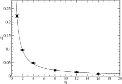
Figure 3: Plot of $\eta$ as a function of $N$ for $T=1.0$. The data fit very well to the form $\eta=0.169(6)/N+0.050(9)/N^{2}$ with $\chi^{2}$/d.o.f$=1.2$.

Figure 4: Plot of $\eta$ as a function of $T/T_{c}$ for various values of $N$.

With regards to the $N$ dependence of our results we find two interesting obervations. Witten argued that when the symmetry is $U(1)$ the large $N$ analysis is still applicable since $\eta\sim 1/N$ at large $N$ [7]. Our results for a fixed $T=1.0$, shown in figure 3, do agree with his conjecture. Interestingly, as $N$ becomes large and $T/T_{c}$ is held fixed instead of $T$, we find that $\eta\neq 0$ even in the large $N$ limit. Figure 4 shows that $\eta$ approaches an interesting function of $T/T_{c}$ as $N$ becomes large. Extending this observation to QCD, we think that the t’Hooft limit (large $N$ with $g^{2}N$ held fixed) may be quite similar [8].

3 Summary

We presented high precision results from simulations of $(2+1)d$ $U(N)$ strongly coupled lattice gauge theories at $T\neq 0$ and we showed convincing evidence that the models undergo a BKT phase transition. In addition, we showed that this universality class is unaffected even in the large $N$ limit, implying that the mean field analysis often used in this limit breaks down in the critical region.

References

- [1] N. Kawamoto and J. Smit, Nucl. Phys. B192 (1981) 100; H. Klumberg-Stern, A. Morel and B. Petersson, Nucl. Phys. B215 (1983) 527; P.H. Damgaard, N. Kawamoto and K. Shigemoto, Phys. Rev. Lett. 53 (1984) 527.
- [2] P. Rossi and U. Wolff, Nucl. Phys. B248 (1984) 105.
- [3] D.H. Adams and S. Chandrasekharan, Nucl. Phys. B662 (2003) 220.
- [4] S. Chandrasekharan and C.G. Strouthos, hep-lat/0306034.
- [5] V.L. Berezinski, Sov. Phys. JETP 34 (1971) 610; J.M. Kosterlitz and D.J. Thouless, J. Phys. C6 (1973) 1181.
- [6] K. Harada and N. Kawashima, J. Phys. Soc. Jpn. 67 (1998) 2768; S. Chandrasekharan and J.C. Osborn, Phys. Rev. B66 (2002) 045113.
- [7] E. Witten, Nucl. Phys. B145 (1978) 110.
- [8] G. t’Hooft, Nucl. Phys. B72 (1974) 461.