On the scaling of computational particle physics codes on cluster computers

Abstract

Many appplications in computational science are sufficiently compute-intensive that they depend on the power of parallel computing for viability. For all but the “embarrassingly parallel” problems, the performance depends upon the level of granularity that can be achieved on the computer platform.

Our computational particle physics applications require machines that can support a wide range of granularities, but in general, compute-intensive state-of-the-art projects will require finely grained distributions. Of the different types of machines available for the task, we consider cluster computers.

The use of clusters of commodity computers in high performance computing has many advantages including the raw price/performance ratio and the flexibility of machine configuration and upgrade. Here we focus on what is usually considered the weak point of cluster technology; the scaling behaviour when faced with a numerically intensive parallel computation. To this end we examine the scaling of our own applications from numerical quantum field theory on a cluster and infer conclusions about the more general case.

1 Introduction

A compute-intensive application might have to be distributed over many compute nodes in order for it to run at a viable speed. One needs to know how well a platform can support the required level of granularity. In this paper we examine this in the case of cluster computers.

The use of clusters of computers in high performance computing has achieved some success with the price/performance advantage of using low-cost and yet high-speed commercial off-the-shelf (COTS) processors to build a fast machine with the budget available. The significant presence of clusters in the TOP500 list [1] attests to the power of this approach.

Cluster computers are also becoming more widely accepted with the growing ease with which they can be configured and maintained; there are now numerous open source and commercial “Cluster in a box” packages available. It can also be important that portable application code can be developed and run on these machines, using standard operating systems, libraries, tools and parallel APIs.

Essential for the use of clusters in many areas of high performance computing is the presence of high performance system area network technology. The question is whether this is good enough to make parallel computation on clusters viable in the face of very fast communications built into MPP or SMP/NUMA machines.

In this paper we intend to make some quantitative statements on the subject by examining the scaling of some codes from our parallel application, viz. Lattice QCD. In section 2 we give a brief description of Lattice QCD, emphasising the computational task involved. Then in section 3 we describe how our code implements this with particular reference to the parallelisation. We proceed to describe in section 4 the scaling tests we apply and present their results. These are summarised and discussed in section 5, after which we present our conclusions.

2 Lattice QCD

Lattice QCD is a numerical evaluation of Quantum Chromodynamics, the theory of the strong interaction, which takes its name from the use of a four-dimensional hypercuboid lattice to represent a discretised spacetime (see e.g. [2, 3] for a recent overview of the subject). In the lattice theory, each lattice site (vertex of the lattice) represents a spacetime point.

These computations are demanding enough that they routinely make much use of supercomputers, and the grid-based formulation of the problem makes it most suitable for data decomposition on parallel machines.

One of the central defining features of a Lattice QCD calculation is the discretised representation of the Dirac fermion operator which describes the interaction of quarks in the theory. On the lattice, the discretised operator takes the form of a fermion matrix. The algorithms used for Lattice QCD calculations are such that the bulk of the computer time is spent in the inversion of this matrix. There is a variety of representations of the fermion matrix which have different properties on the lattice but they should all become identical to the continuum Dirac operator in the limit of zero lattice spacing. The particular formalism used in this work is that originally due to Wilson [4]. The Wilson fermion matrix is

$$M_{xy}=\delta_{xy}-\kappa D_{xy}$$ (1)

where the indices $x$ and $y$ refer to lattice sites and $\kappa\in\mbox{\bb\char 82\relax}$ is the hopping parameter, related to the bare quark mass.

The Wilson hopping matrix is

$$D_{xy}=\sum_{\mu=0}^{3}(1-\gamma_{\mu})U_{\mu\,x}\delta_{y\,x+\hat{\mu}}+(1+\gamma_{\mu})U_{\mu\,x-\hat{\mu}}^{\dagger}\delta_{y\,x-\hat{\mu}}$$ (2)

where the lattice gauge fields $U_{\mu\,x}\in SU(3)\subset\mbox{\bb\char 67\relax}^{3\times 3}$ carry colour indices and the Dirac $\gamma$-matrices $\gamma_{\mu}\in\mbox{\bb\char 67\relax}^{4\times 4}$: $\{\gamma_{\mu},\gamma_{\nu}\}=2\delta_{\mu\nu}$ carry spin indices.

Therefore $M$ is a matrix in lattice site $\otimes$ spin $\otimes$ colour space. If the number of sites in the lattice is $V$ then the fermion matrix is a complex matrix of size $(12V)^{2}$ acting on vectors consisting of $12V$ complex numbers.

The lattice is of finite extent, and we impose periodic or antiperiodic boundary conditions.

Note that the lattice site structure of this matrix is either local or connects nearest-neighbour sites. Therefore it is a sparse matrix and is implemented as an operator rather than stored explicitly

Other formulations of the fermion matrix include the Sheikholeslami-Wohlert discretisation which adds to the Wilson matrix a $3\otimes 4\times 3\otimes 4$ complex matrix diagonal in lattice sites [5] , variations of the Kogut-Susskind matrix [6] which have no spin components but can have a more than nearest-neighbour connectivity [7, 8] and the Fixed Point formulations which have spin and colour indices and more than nearest-neighbour connectivity [9]. The choice depends on the desired properties, and has consequences for the balance of computation to communication required; for example, the Sheikoleslami-Wohlert matrix has more local computation than the Wilson matrix with no extra communication and will therefore scale better.

The Wilson matrix has the favourable property of only requiring nearest-neighbour communications but since its computational requirements are comparatively modest it does put some pressure on the scaling abilities of a parallel machine. Although it is one of the older formulations it is still interesting not least because it can be used as the basis for the new breed of Ginsparg-Wilson lattice fermion formulations [10, 11], which have very favourable field-theoretic properties but are still very expensive to compute with; a single multiplication by the GW fermion matrix involves many ($\mathcal{O}(100)$) multiplications by the Wilson matrix. For these reasons we believe that our test results with the Wilson matrix are relevant. However we also consider the effects of a fermion matrix requiring more than nearest-neighbour communications.

3 Description of Lattice QCD software

We give here some details of the implementation of our lattice QCD applications, describing the computational task itself, how the code is written and how the code is parallelised.

Much of the code used in these tests was actually developed for a specific Lattice QCD project called GRAL  [12]. The GRAL project has as its aim the finite size scaling analysis of QCD physics close to the chiral regime of light dynamical quarks using the Wilson formulation. This requires a large computational effort, and although a cluster is just one of the machines that is used for the project, good performance of the Lattice QCD code on it is important to the project’s success.

The bulk of the code is written in C compiled with the Compaq C Compiler ccc with a set of optimisations enabled with the -fast flag. We use assembly language kernels [13] for certain low-level numerically intensive routines where performance is critical. Routines from the optimised BLAS library are also used where appropriate. Both 32-bit and 64-bit code is implemented, but since 64-bit accuracy is preferred for the GRAL project, we present here only 64-bit results.

The communications are entirely handled with message passing via MPI. The fast MPI-library on ALiCE is provided by the ParaStation™ cluster middleware [20].

3.1 Fermion matrix inversion

As stated in section 2 most computer time will be spent in those portions of this code which invert the fermion matrix. This involves solving the linear system

$$M\psi=b$$ (3)

where $M$ is the fermion matrix defined in section 2, $b$ is the source vector and $\psi$ is the solution to be found. A Krylov subspace algorithm is best suited to the solution of such a sparse linear system. We have implemented several such algorithms but here we show results using the BiCGStab [14, 15] method which is usually the fastest. The communication requirements (described in section 3.3) of these different algorithms are comparable.

An additional refinement is the use of a parallel (locally lexicographic) SSOR preconditioning [16, 17] to reduce the number of iterations of the BiCGStab solver. This requires a slightly different pattern of communication and so we present these results separately.

3.2 Grid decomposition

The four-dimensional lattice is decomposed over a grid of processing nodes. This grid can be from zero dimensions (i.e., a single node) to four dimensions (since the lattice is four-dimensional). The number of nodes along any dimension is restricted in that the local lattice on each node must have identical size and shape. This constraint is not strictly necessary on a MIMD machine but it makes the implementation simpler and ensures perfect load balancing.

3.3 Nearest-neighbour communication requirements

Every iteration of the solver algorithm requires three global summations of a complex number and performs two multiplications by the fermion matrix.

Each fermion matrix multiplication requires nearest-neighbour communication of the multiplicand vector. On a lattice boundary in a non-parallelised direction this is taken care of by the boundary condition. In a parallelised direction the required data is on another node. With the message passing communication paradigm, this means that the data on those lattice sites on the boundary of a local lattice is sent to the neighbouring node. Each node receives data from neighbouring nodes and stores it in buffers. This communication pattern is illustrated in figure 1.

The amount of data to be sent depends on the size of the lattice and the grid decomposition. If these are such that on each node of a grid of dimensionality $d>0$ the local lattice has $V$ sites, then the number of sites on the boundaries from which data must be sent is

$$2V\sum_{\mu=0}^{d-1}\frac{1}{N_{\mu}},$$ (4)

where the sum is over parallelised directions $\mu$ and $N_{\mu}$ is the length of the local lattice in direction $\mu$. Recall that a vector consists of 12 complex numbers on each lattice site, which is 192 bytes at 64-bit precision.

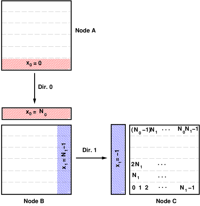
Figure 1: An illustration of the nearest-neighbour communications in two dimensions of a two-dimensional local lattice of size $N_{0}\times N_{1}$. Nodes A and B show the communication in a 1-dimensional processor grid in the negative direction 0: The data on Node A with coordinate $x_{0}=0$ is copied to a buffer on Node B where it can be accessed as Node B data with coordinate $x_{0}=N_{0}$. The positive direction 0 communication is analogous. Nodes C and B show the communication in a 2-dimensional grid in the positive direction 1: The data on Node B with coordinate $x_{1}=N_{1}-1$ is copied to a buffer on Node C where it can be accesssd as local data with coordinate $x_{1}=-1$. The negative direction 1 communication is analogous. Each node sends data in this way from all its boundaries.

For the normal BiCGStab algorithm all the data on a boundary can be sent at once as a single message. We send each boundary before the multiplication by the fermion matrix begins. The order in which they are sent is essentially unimportant.

The SSOR preconditioning requires most of the data to be sent incrementally as a succession of smaller messages at various points within the matrix-vector multiplication; the order is important. This arrangement is potentially less favourable because of a possibly inefficient use of available bandwidth and the effect of multiple latency penalties.

3.3.1 Data layout

The parallelisation efficiency is affected by the way the data is stored along with the design of the communication buffers.

The vectors involved in the calculation are stored as site-major arrays. Each array element contains the 12 complex numbers and the $n-$th element corresponds to the local lattice site with cartesian coordinates $(x_{0},x_{1},x_{2},x_{3})$ via $n=x_{3}+N_{3}x_{2}+N_{3}N_{2}x_{1}+N_{3}N_{2}N_{1}x_{0}$ where $N_{\mu}$ is the size of the local lattice in the $\mu$th direction. The gauge fields are stored in a similar way.

This storage order is illustrated in figure 1. Note that because of the layout of the data in lattice, the data on the direction 1 boundaries is strided, which takes more time to copy than contiguous data.

The communication buffers are, for convenience, attached to this array, which increases its length by an amount the size of the local lattice boundaries. Two arrangements of the buffers were tried:

The “halo” layout

The “halo” layout places the buffers on either side of the array body, e.g. for a local lattice of size $N_{0}\times N_{1}\times N_{2}\times N_{3}$, the first two buffers would be

$x_{1}=-1$$x_{0}=-1$$n=0\cdots N_{0}N_{1}N_{2}N_{3}-1$$x_{0}=N_{0}$$x_{1}=N_{1}$

The “tail” layout

An alternative is the “tail” layout:

$n=0\cdots N_{0}N_{1}N_{2}N_{3}-1$$x_{0}=-1$$x_{0}=N_{0}$$x_{1}=-1$$x_{1}=N_{1}$

where the buffers are attached to the end of the array. In section 4.4.1 we test the differences between these two layouts.

3.4 Next-to-nearest-neighbour communication
requirements

Although the Wilson fermion matrix requires only nearest-neighbour communication of the gauge field $U$, for algorithmic reasons we also need next-to-nearest-neighbour access.

Furthermore, as mentioned in section 1, some fermion matrices connect more than nearest-neighbour lattice sites. We investigate the effects of this by considering next-to-nearest-neighbour communication. This is already possible on a 1-dimensional grid with the communication patterns already presented, but on a 2-dimsional grid the communication in direction 1 has to be changed as shown in figure 2. Additional data from the corners of the lattices has to be sent.

For a lattice with $V$ sites on each node of a grid of dimensionality $d>1$, there are

$$4V\sum_{\mu=0}^{d-1}\sum_{\nu=0}^{\mu-1}\frac{1}{N_{\mu}N_{\nu}}$$ (5)

lattice sites on the corners from which data must be sent, where the sum is over parallelised directions $\mu$ and $\nu$ and $N_{\mu}$ and $N_{\nu}$ are the lengths of the local lattice in those directions. This is in addition to the amount of boundary data described in section 3.3. We wish to test the effect of this additional communication.

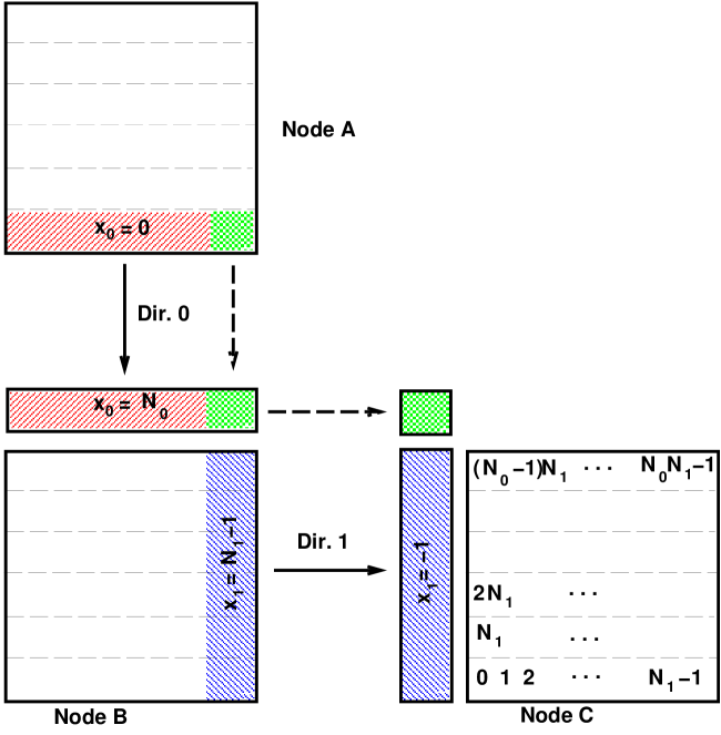
Figure 2: An illustration of next-to-nearest-neighbour communications in two dimensions of a two-dimensional local lattice of size $N_{0}\times N_{1}$. In addition to the data communications shown in figure 1 the corner of the node A lattice (coordinates $x_{0}=N_{0}$, $x_{1}=N_{1}-1$) is sent to a buffer on node C where it can be accessed as data with coordinates $x_{1}=-1$, $x_{0}=-1$. We do this in two stages, sending the data via the $x_{0}=N_{0}$ buffer of node B, so the direction 0 communication must complete before the direction 1 communication can start. Blocking or semi-blocking semantics are suitable here. An alternative (not examined here) would be to send the corner from node A directly to node C, which in principle avoids this wait.

3.4.1 Data layout

The next-to-nearest neighbour communication pattern in more than one dimension requires extra buffers on each array for the corner data. The possibilities for different data layouts are therefore increased. We illustrate three possibilities for the layout on a two-dimensional grid (which can be generalised for a greater number of dimensions):

Layout 0

The corner buffers are added as halos to the $x_{1}=-1$ and $x_{1}=N_{1}$ buffers;

$x_{1}=-1,x_{0}=-1$$x_{1}=-1$$x_{1}=-1,x_{0}=N_{1}$

$x_{0}=-1$$n=0\cdots N_{0}N_{1}N_{2}N_{3}-1$$x_{0}=N_{0}$

$x_{1}=N_{1},x_{0}=-1$$x_{1}=N_{1}$$x_{1}=N_{1},x_{0}=N_{1}$

layout 1

The corner buffers are added to the $x_{1}=-1$ and $x_{1}=N_{1}$ buffers as tails;

$n=0\cdots N_{0}N_{1}N_{2}N_{3}-1$$x_{0}=-1$$x_{0}=N_{0}$

$x_{1}=-1$$x_{1}=-1,x_{0}=-1$$x_{1}=-1,x_{0}=N_{1}$

$x_{1}=N_{1}$$x_{1}=N_{1},x_{0}=-1$$x_{1}=N_{1},x_{0}=N_{1}$

layout 2

The corner buffers are added as a tail at the end of the array;

$n=0\cdots N_{0}N_{1}N_{2}N_{3}-1$$x_{0}=-1$$x_{0}=N_{0}$$x_{1}=-1$$x_{1}=N_{1}$

$x_{1}=-1,x_{0}=-1$$x_{1}=-1,x_{0}=N_{1}$$x_{1}=N_{1},x_{0}=N_{1}$$x_{1}=N_{1},x_{0}=-1$

Layouts 0 and 1 have the advantage that the data in the $x_{0}=N_{0}$ and $x_{0}=-1$ buffers with $x_{1}=0\;(N_{1}-1)$ can be sent in the negative (positive) direction 1 along with the data with $0\leq x_{0}<N_{0}\mbox{, }x_{1}=0\;(N_{1}-1)$ as a single message.

Layout 2 requires that the corners buffers be sent seperately. However, since it is merely the tail layout of section 3.3.1 with extra buffer space added to the end of it, a single layout can be used for fields both with and without next-to-nearest-neighbour interaction without wasting space.

4 The scaling tests

Our goal is to test how well the code introduced in section 3 scales on a cluster. We run tests to see how this is affected by various factors; the data layout, the locality of the fermion matrix and the solver algorithm.

In this section we first describe the essential details of all the scaling tests. We then describe the hardware and software on which these tests are run.

4.1 The test specifications

In order to test the scaling of our lattice QCD applications, we choose to test the fermion matrix inversion described in section 3.1 since it is the area in which many QCD programs and in particular the GRAL applications will spend most run-time and it has the considerable communication requirements discussed in section 3.3. All the tests are run in 64-bit precision.

We choose to time the inversion on a $12^{4}$ lattice. This rather arbitrary size is smaller than that used in most realistic lattice QCD calculations. As our machine size is 128 processors, this lattice size should give an idea of how the performance is affected by the size and surface/volume ratio of the sub-lattices on each node when extrapolated to larger computers with 512 or 1024 processors.

Each solve is performed on a random $SU(3)$ gauge field with a random gaussian source vector. The solve is repeated many times until a good estimate of the average run-time per solve can be obtained. The run-time on a single node is very well reproducible, but on multiple nodes there is some variation, perhaps due to effects of different physical grid topologies or the load on the network and switches, so the entire run is repeated at least five times to average over such variations.

Table 1 shows the grid topologies used in the tests. Results from grids of the same dimensionality and number of nodes are averaged. The ratio of the communicable surface of the local lattice to the local lattice volume is also shown.

nodes	grid	local lattice	surface/volume
2	$2\times 1\times 1\times 1$	$6\times 12\times 12\times 12$	0.33
3	$3\times 1\times 1\times 1$	$4\times 12\times 12\times 12$	0.50
4	$4\times 1\times 1\times 1$	$3\times 12\times 12\times 12$	0.67
6	$6\times 1\times 1\times 1$	$2\times 12\times 12\times 12$	1.00
12	$12\times 1\times 1\times 1$	$1\times 12\times 12\times 12$	2.00
4	$2\times 2\times 1\times 1$	$6\times 6\times 12\times 12$	0.67
9	$3\times 3\times 1\times 1$	$4\times 4\times 12\times 12$	1.00
12	$4\times 3\times 1\times 1$	$3\times 4\times 12\times 12$	1.17
12	$3\times 4\times 1\times 1$	$4\times 3\times 12\times 12$	1.17
16	$4\times 4\times 1\times 1$	$3\times 3\times 12\times 12$	1.33
36	$6\times 6\times 1\times 1$	$2\times 2\times 12\times 12$	2.00
8	$2\times 2\times 2\times 1$	$6\times 6\times 6\times 12$	1.00
27	$3\times 3\times 3\times 1$	$4\times 4\times 4\times 12$	1.50
36	$3\times 3\times 4\times 1$	$4\times 4\times 3\times 12$	1.67
64	$4\times 4\times 4\times 1$	$3\times 3\times 3\times 12$	2.00
16	$2\times 2\times 2\times 2$	$6\times 6\times 6\times 6$	1.33
36	$2\times 3\times 3\times 2$	$6\times 4\times 4\times 6$	1.67
64	$2\times 4\times 4\times 2$	$6\times 3\times 3\times 6$	2.00

Table 1: The grid sizes, local lattice sizes and local lattice surface/volume ratios used in the scaling measurements. The global lattice size is $12^{4}$ throughout our tests.

Our main metric of the parallel performance is the speedup;

$$\mbox{speedup}=\frac{\mbox{speed on {n} nodes}}{\mbox{speed on 1 node}}.$$ (6)

It can also be useful to know the parallel efficiency (scaled speedup);

$$\mbox{parallel efficiency}=\mbox{scaled speedup}=\frac{\mbox{speedup}}{\mbox{{n}}}.$$ (7)

4.2 The test platform

ALiCE, the Alpha-Linux Cluster Engine at Wuppertal University is a general purpose high-performance computer consisting of 128 Compaq DS10 servers, each with a 616MHz Alpha 21264 processor, 64 kB 2-way set-associative level 1 data and instruction caches and a 2 MB level 2 cache [18]. The Alpha 21264 is 4-way superscalar, sustaining 2 floating-point operations per cycle. The operating system is SuSE Linux [19].

ALiCE is clustered using Myrinet with the ParaStation3 cluster middleware[20]. This arrangement takes advantage of the open architecture of the Myrinet communication hardware to replace the standard firmware supplied by Myricom with that supplied by Par-Tec, together with kernel extensions and communications libraries. The ParaStation system endeavors to achieve high performance by implementing a reliable communications protocol in firmware and keeping communications in user space. The two-way 1.28 Gbit/s Myrinet network is configured as a multistage crossbar and the Myrinet cards have a 64 bit/33 MHz PCI buses. We use MPICH 1.2.3 as the interface between our application code and the ParaStation middleware. On ALiCE, the latency for ParaStation/MPI is $16\mu$s; the bi-directional bandwidth is about 170 MB/s [21].

4.3 Single node performance

In evaluating the following results it will be helpful to know the performance of the solvers on a single node. Figures 3 and 4 show how the speed of the BiCGStab solver and the SSOR preconditioned BiCGStab solver vary with the number of sites in the lattice. Memory cache and memory bandwidth effects mean that performance deteriorates as the lattice volume increases.

Figure 3: The speed of the BiCGStab solver on a single node as a function of the lattice volume. The corresponding lattice dimensions are indicated along the top.

Figure 4: The speed of the SSOR preconditioned BiCGStab solver on a single node as a function of the lattice volume. The corresponding lattice dimensions are indicated along the top.

BiCGStab sustains a speed of 237 Mflops on our $12^{4}$ test lattice described in section 4.1, while SSOR preconditioned BiCGStab sustains a speed of 220 Mflops. The latter solver is preferred because it still finds the solution faster due to the smaller number of iterations.

4.4 The results of the scaling tests

We now examine what happens to the performance of our solvers as we move from a serial to a parallel implementation. There are numerous factors which might affect the parallel performance; we make a preliminary investigation into the effects of data layout and communication semantics before presenting our final results for the speedup and parallel efficiency.

4.4.1 Investigation of data layout

We compare how the two data layouts described in section 3.3.1 affect the scaling of the data. It might be expected that the halo layout would have better spatial locality properties (and therefore use the cache better), but the performance, shown in figure 5, seems to be much the same. This could be because of the data prefetching written into our assembler kernels.

Figure 5: The speedup of the BiCGStab solver using nearest-neighbour blocking communications on one- and two-dimensional grids, comparing the data layouts described in section 3.3.1.

We choose to use the tail format. It is easily adapted to the case of next-to-nearest-neighbour communications (which we need for the gauge field) by simply adding extra buffer space at the end of the array.

4.4.2 Investigation of communication semantics

We can hope to improve performance using non-blocking (asynchronous) communications (e.g MPI_Isend) rather than blocking (synchronous) communications (e.g MPI_Send).

Figure 6 shows that this improves BiCGStab performance on a 1-dimensional grid but degrades it on a 2-dimensional grid. We try a semi-blocking approach where non-blocking communications are used in direction 0, then a block allows this communication to complete before non-blocking communications are used in direction 1; this aproach does not work either. We have verified that this is also the case for grids of dimension greater than 2. Henceforth with BiCGStab we use non-blocking communications on one-dimensional grids and blocking communications on grids of more than one dimension.

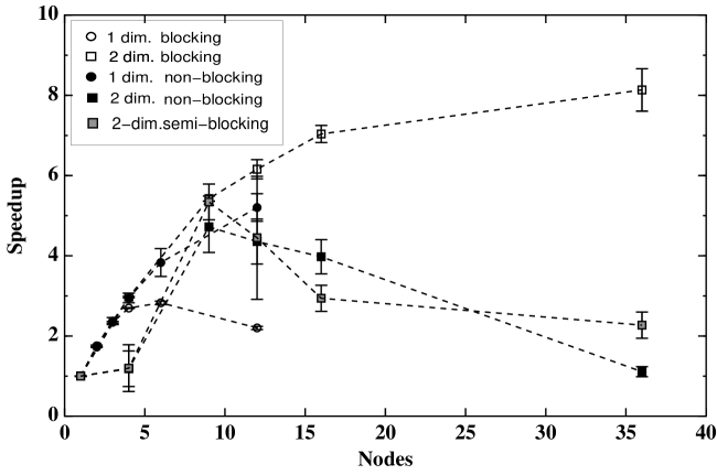
Figure 6: The speedup of the BiCGStab solver comparing nearest-neighbour blocking and non-blocking communications.

Figure 7 shows that the situation is different with SSOR preconditioned BiCGStab: non-blocking communications are faster even on the two-dimensional grid. Henceforth we use non-blocking communications in connection with SSOR preconditioned BiCGStab. We suspect that the communication of BiCGStab, where long messages are sent, might negatively interfere with caching and compute processes. A better separation of communication directions with smaller message lengths, as is the case for SSOR, might lead less often to a situation in which data used for compute operations competes for cache lines with data used simultaneously for communication

Figure 7: The speedup of the SSOR preconditioned BiCGStab solver comparing nearest-neighbour blocking and non-blocking communications.

4.5 Results for solver speedup and parallel efficiency

Having determined that the data layout is not very significant and when it is better to use blocking or non-blocking communications, we can present the results for the best scaling of our solvers on one- to four-dimensional grids.

Figure 8: The speedup of the BiCGStab solver.

Figure 9: The parallel efficiency of the BiCGStab solver.

Figure 10: The speedup of the SSOR preconditioned BiCGStab solver.

Figure 11: The parallel efficiency of the SSOR preconditioned BiCGStab solver.

What we see is that for the BiCGStab solver on this test lattice (figures 8 and 9) the one- and two-dimensional grids become quite inefficient on more than a few nodes. On the three- and four-dimensional grids the drop in efficiency on large numbers of nodes is not as dramatic; a reasonable speedup is achieved due to the more favourable surface/volume ratio. The speedup on a four-dimensional grid is not convincingly better than that on a three-dimensional grid, presumably because the data on the direction 3 boundaries is so finely strided as to negate the advantage of better surface/volume ratios.

The SSOR results (figures 10 and 11) show that the speedup is less affected by the dimensionality of the grid i.e. the surface/volume ratio. However the fact that the data on the direction 3 boundaries are so finely strided adversely affects the four-dimensional grid performance, since in this case it means that very many send/receives have to be done, which is evidently too inefficient due to latency effects.

A main result of these investigation is that a small $12^{4}$ lattice still performs with a scaled speedup of 0.45 on 64 processors. We will comment on this in section 5.1.

To shed further light on these results we plot in figures 12 and 13 the percentage of the total wall-clock execution time required for communication against the ratio of the communicable surface of the local lattice to the local lattice volume. The correlation does not usually depend very strongly on the dimensionality of the grid; a notable exception is the SSOR preconditioned solver on the four-dimensional grids. Note also how the dependence is weaker when the solver is SSOR preconditioned.

Figure 12: The dependence of the percentage of BiCGStab run-time spent in communication on the surface/volume ratio of the local lattice.

Figure 13: The dependence of the percentage of SSOR preconditioned BiCGStab run-time spent in communication on the surface/volume ratio of the local lattice.

4.6 Results for next-to-nearest-neighbour communication

We examine the overhead introduced by the need to send the extra data from the boundary corners by implementing next-to-nearest-neighbour communications and timing exactly the same BiCGStab solve of the same fermion matrix as before on two-dimensional grids. Any difference is therefore entirely due to the extra comunication. Again it was found that for BiCGStab, blocking communications were fastest, so these tests are performed with blocking communications.

4.6.1 Investigation of data layout

We compare in figure 14 the three layouts defined in section 3.4.1. Because of the seperate messages required, the third layout is the least scalable, but the differences only become significant in the region of poor scaling. Because of this and the fact that for our applications the next-to-nearest-neighbour communications are relatively unimportant, we adopt the third layout for the gauge field in the GRAL code, utilising the benefits of a unified data layout as described in section 3.4.

Figure 14: The speedup of the BiCGStab solver using next-to-nearest-neighbour blocking communications on two-dimensional grids, comparing the data layouts described in section 3.4.1.

4.6.2 Results for the speedup

In figure 15 we take the most scalable next-to-nearest-neighbour layout and compare its speedup with the nearest-neighbour communications on a two-dimensional grid, demonstrating the effect of sending the extra data from the corners of the lattice.

This is perhaps a favourable comparison since the amount of extra data that must be sent for next-to-nearest-neighbour communications increases with the dimensionality $d$ of the node grid as described in section 3.4

Figure 15: The speedup of the BiCGStab solver using nearest- and next-to-nearest-neighbour blocking communications on two-dimensional grids

5 Summary and conclusions

We have presented the results of tests of the scaling of the Wilson matrix solver for a $12^{4}$ test lattice on ALiCE . Here we summarize those results and discuss their implications.

5.1 Summary

On small numbers of nodes the BiCGStab solver scales without much dependence on the grid decomposition. If a minimum effiency of 75% percent is demanded then figure 9 indicates that no more than 4 nodes should be used. However it still maintains around 50% efficiency on about 16–36 nodes on a three- or four-dimensional grid, corresponding to local lattices of $6^{4}$–$4^{2}\times 6^{2}$ or surface/volume ratios of 1.33–1.67. Thereafter the efficiency degrades, but not too sharply.

The SSOR preconditioned solver has similar small grid characteristics; figure 11 suggests that the 75% efficiency bound is reached at around 4–9 nodes. The four-dimensional grids rapidly become very slow but an efficiency of around 50% is maintained on two and three-dimensional grids of around 36 nodes, i.e. a $4\times 4\times 3\times 12$ local lattice with surface/volume ratio 1.67 or a $2^{2}\times 12^{2}$ lattice with surface/volume ratio 2.00. The performance degrades slowly thereafter; we still have 45% efficiency on 64 nodes with a $3^{3}\times 12$ local lattice.

That the scaling performance need not be seriously affected by the data layout is a heartening result for code developers; we are free to organise data in whichever way is convenient.

A curious feature of our system is the performance of the non-blocking communications. It appears that if the communications in different directions are well separated then non-blocking semantics are an improvement. But they are a hindrance if those communications are done at the same time, even when separated by an explicit barrier as in the semi-blocking case. We have argued above that cache effects might be responsible for these differences.

One gratifying result is how well the SSOR preconditioned solver scales. Its algorithmic performance is excellent but its more complicated pattern of communication can in practice lead to scaling problems due to the communication latency. The vice of needing many smaller messages rather than a few large ones appears to become a virtue, since the separation of sends allows the faster non-blocking communications to be used. This demonstrates that a more complicated algorithm need not be deleterious to efficiency and performance.

5.2 Discussion

We see that in general the scaling ability is limited by the additional time that has to be used for the communications and this is essentially determined by the surface/volume ratio. Therefore the results presented here can serve as a guide for planning future runs on realistic lattices of larger global size, bearing in mind that increasing the global size introduces additional overheads from the collective communications.

For example, the discussion in the previous section concluded that our $12^{4}$ lattice runs with 75% efficiency on 4 nodes with BiCGstab. According to table 1 this corresponds to a surface/volume ratio of $\frac{2}{3}$. Therefore if we require 75% efficiency on any lattice we should aim for grid decomposition which gives a local surface/volume ratio of about $\frac{2}{3}$. From equation (4) we obtain the constraint on the dimensions of the local lattice in parallel directions

$$\sum_{\mu=0}^{d-1}\frac{1}{N_{\mu}}\simeq\frac{1}{3}.$$ (8)

This is achieved for a $12^{3}\times 24$ lattice with a grid of $1\times 2\times 2\times 2$ (8 processors) or possibly $1\times 1\times 2\times 6$ (12 processors). A $16^{3}\times 32$ lattice needs a $1\times 2\times 2\times 2$ (8 processors) or $1\times 2\times 2\times 4$ (16 processors) grid. A $24^{3}\times 48$ lattice needs a $2\times 2\times 2\times 4$ (32 processors) grid.

With SSOR preconditioning we might be able to use 1.0 as a target surface/volume ratio, and use grids of $1\times 2\times 2\times 4$ (16), $1\times 2\times 4\times 4$ (32) and $1\times 4\times 4\times 4$ (64) respectively. A similar analysis suggests that a lattice of size $24^{4}$ can be expected to run with a scaled efficiency of about 0.45 on 512 processors.

While there must be an optimum grid decomposition for a given problem and problem size, the complicated nature of the relationship between latency, bandwidth and message length makes finding this “sweet spot” a difficult optimisation problem.

In general there is a trade-off between speed and efficiency which must be determined according to the needs of each project and the resources available; one would also take into account the single-node speed when deciding the local lattice size.

The GRAL project typically requires a number of concurrent simulations at different physical parameters which will run for some considerable length of time. The former requirement will probably mean using a modest number of nodes on ALiCE for each run, it being a shared multi-purpose facility, and the latter requirement will favour running at a reasonable efficiency. Fortunately these considerations are entirely compatible and we have shown here that the required performance is available. We also now know that should a run need to proceed at greater speed, albeit less efficiently, then this is also feasible.

The target surface/volume ratio will in general change when a different sort of fermion matrix is used. Our measurements indicate that a fermion matrix with next-to-nearest-neighbour communications might introduce an additional communications overhead of about 10%.

5.3 Outlook

It is reasonable to speculate about what these results mean, or how they would change, for future cluster computer platforms. A faster CPU will increase the proportion of time spent in communications relative to computation, but it should be remembered that a faster CPU will speed up the communications too, so the overall effect might not be too different.

One should be aware that network and communications technology is also developing: we can look forward to high-bandwidth PCI buses and faster networks [22, 23]. In fact much of this technology exists already, and as cluster computing becomes more widespread and new network standards (e.g. InfiniBand) become available, current higher-performance technologies (e.g. Gigabit System Network) will become affordable.

A greater network speed helps scalability, but also of importance for the developer, in that it could change the way application code is designed, are implementations of communications APIs that make good use of DMA technology to provide support for simultaneous sends/receives of messages to multiple nodes, or for overlapping communications with computations.

Of great importance to performance of scientific codes are factors like data cache sizes and memory bandwidths. If these are greater then it is more difficult to achieve efficient scaling, but the benefits to the performance on each node might make decomposition still worthwhile. Conceivably, there could then be a situation where a finer grained decomposition actually improves speedup by moving into a régime where all local data fit into cache.

References

- [1] http://www.top500.org
- [2] R. Gupta; Parallel Computing 25 (1999) 1199 (hep-lat/9905027) and references therein.
- [3] C. Davies, in Heavy Flavour Physics; Scottish Graduate Textbook Series, Institute of Physics 2002, eds C. T. H. Davies and S. M. Playfer hep-lat/0205181
- [4] K. G. Wilson, in New Phenomena in Subnuclear Physics, ed. A. Zichichi (Plenum, New York, 1977)
- [5] B. Scheikholeslami and R. Wohlert; Nucl. Phys. B 259 (1985) 572
- [6] J. Kogut and L. Susskind; Phys. Rev. D 11 (1975) 395
- [7] K. Originos et al.; Phys. Rev. D 60 (1999) 054503 (hep-lat/9903032)
- [8] J-F. Lagaë and D. K. Sinclair; Phys. Rev. D 59 (1999) 014511 (hep-lat/9806014)
- [9] P. Hasenfratz; Nucl. Phys. (proc. suppl.) B 63 (1998) 53 (hep-lat/9803027) and references therein.
- [10] D. B. Kaplan; Phys. Lett. B 288 (1992) 342
- [11] R. Narayanan and H. Neuberger; Nucl. Phys. B 433 (1995) 305
- [12] B. Orth et al.; Nucl. Phys. (proc. suppl) 106 (2002) 289 (hep-lat/0110158)
- [13] http://www.theorie.physik.uni-wuppertal.de/Computerlabor/Alice/akmt.phtml
- [14] H. A. Van der Vorst; SIAM J. Sci. Stat. Comp. 13 (1992) 631
- [15] A. Frommer et al.; Int. J. Mod. Phys. C 5 (1994) 1073
- [16] S. Fischer et al.; Comp. Phys. Comm. 98 (1996) 20
- [17] Th. Lippert; Parallel Computing 25 (1999) 1357
-
[18]
N. Eicker et
al.; Nucl. Phys. (proc. suppl.) B 83 (2000) 798 (hep-lat/9909146)
http://www.theorie.physik.uni-wuppertal.de/Computerlabor/ALiCE.phtml - [19] http://www.suse.de
- [20] http://www.par-tec.de
- [21] Th. Düssel et al.; cs.DC/0303016. To be published in Parallel Computing.
- [22] http://www.pcisig.com/specifications/pcix_20
- [23] http://www.infinibandta.org