1 Introduction and summary

QCD spectroscopy with traditional fermion formulations faces some open problems. For a Dirac operator with poor chiral properties the fluctuations of the small eigenvalues limit the minimal bare quark masses one can work at. Wilson fermions have large cut-off effects and years of experience have demonstrated [1, 2] that it is very hard to reach pseudoscalar (PS) masses below 300 MeV in quenched QCD. This problem becomes even worse if the ${\cal O}(a)$-correcting clover term is included [3, 4]. In full QCD the situation does not seem to be improved. State of the art dynamical fermion simulations stay above $m_{\mathrm{PS}}\approx$ 450 MeV [5, 6, 7]. Twisted mass Wilson fermions are an interesting development [8, 9] but need detailed numerical testing. For staggered fermions - after recent progress with reducing the cut-off effects and thus flavor symmetry violation [10, 11, 12] - the main open question is, whether staggered fermions can describe QCD with less than 4 degenerate fermions. The solutions [13] of the Ginsparg-Wilson equation [14] are free of these problems: Exact chiral symmetry [15] kills the dangerous fluctuations which prevent simulations of light pions and they are automatically ${\cal O}(a)$ improved [16].

There exists a large number of studies exploring Dirac operators with chiral symmetry in quenched QCD (for recent reviews, see [17] and references therein). Different aspects of hadron spectroscopy have also been considered in [18, 19, 20] with domain-wall [21] and overlap [22] fermions. However, so far no detailed study has been attempted on spectroscopy with light pions. In this work we explore spectroscopy down to $m_{\mathrm{PS}}/m_{\mathrm{V}}=0.28$ using two Dirac operators based on the Ginsparg-Wilson equation: the parametrized fixed-point (FP) and the chirally improved (CI) Dirac operators. Actions with exact chiral symmetry are expensive to simulate. Our approach is a compromise trying to reduce the cost under the condition of being able to reach pion masses where chiral perturbation theory can be safely and effectively used for extrapolation. For comparison, at one lattice spacing and lattice size, we simulated also an approximate overlap Dirac operator obtained from the FP Dirac operator, by performing a Legendre expansion of order 3 to approximate the overlap projection. Finding the right balance between expense and good physical properties of an action is an important issue. Significantly simpler and less expensive actions were investigated in [23] and [24].

Fixed-point actions result from solving the real space renormalization group equations in the weak coupling limit [25]. After the first attempts in 2 and 4 dimensional models [26], a finite parametrization of FP fermions suitable for numerical calculations has been developed [27, 28] giving rise to an approximate solution of the Ginsparg-Wilson equation. The idea behind the CI operator is a systematic expansion of a solution of the Ginsparg-Wilson equation in terms of simple lattice operators [29]. CI fermions have been shown to give rise to a Dirac operator with good chiral properties both in 2 and 4 dimensions [30].

The goal of our spectroscopy calculations with FP and CI fermions is to explore a new mass region and check whether the promises of chiral symmetry, i.e. small pion masses and good scaling properties, become manifest. The new results also help to outline the effects of finite volume in quenched QCD with light pions. In particular we compare our results for scaling properties with those of recent large-scale simulations using staggered or Wilson fermions [2, 3, 10, 31]. Preliminary results for FP and CI fermions were reported in [32, 33, 34, 35]. A CI calculation of vector meson couplings to vector and tensor currents was presented in [36].

Some of the results of this paper deviate from those presented in our preliminary discussion [33, 34]. Our data analysis is more careful and conservative than before. The statistics is also increased slightly. Most importantly, however, for the FP operator the masses in the decuplet baryon sector have changed mainly due to a corrected bug in the code constructing the decuplet baryon out of quark propagators. The negative parity partner of the nucleon is studied in the present version also.

Let us summarize our main results and give conclusions. Our Dirac operators allow spectroscopy with pseudoscalar masses down to 220 MeV even on coarse lattices with $a=0.15\,\mathrm{fm}$. So close to the chiral limit quenched spectroscopy is heavily contaminated by topological finite size artifacts in all hadronic channels at small and intermediate volumes. It is mandatory to work with hadron operators where these artifacts are cancelled or at least reduced. In the pseudoscalar channel we clearly see the chiral logarithms and tested different methods to determine the chiral log parameter $\delta$. In our large ($L=2.5\,\mathrm{fm}$) volume spectroscopy we argue for using masses of stable particles/narrow resonances as input parameters. The results suggest an intuitive picture where the size of quenching artifacts in the hadron masses is strongly correlated with their experimentally observed widths. (Similar observations have been made earlier in [37].) We find consistency between the scales of the gauge and hadronic sectors. We perform different scaling tests changing the resolution in the range $a=0.08-0.15\,\mathrm{fm}$. No scaling violation is found within our data beyond the statistical errors. Comparing our results with other large scale simulations the conclusion depends on whether the extrapolated CP-PACS data really describe the continuum limit. This is a non-trivial question since the extrapolated continuum result is significantly different from the measured data obtained on the finest lattice at $a=0.05\,\mathrm{fm}$ [2]. If the answer is yes, then the FP action results (and also the CI action results, although within larger statistical errors) at $a=0.15\,\mathrm{fm}$ show cut-off effects, but they are closer to the continuum than the Wilson results at $a=0.05\,\mathrm{fm}$ and the improved staggered results at $a=0.13\,\mathrm{fm}$ and $0.09\,\mathrm{fm}$ and are comparable to the clover improved results at $0.07\,\mathrm{fm}$. We see no finite volume effects above $L=1.8\,\mathrm{fm}$. We remark finally that the codes are easy to parallelize and run well on two supercomputers with different architectures.

In a direct comparison of FP and CI fermions we conclude that in the whole range of parameters we worked at the two operators essentially perform equally well in light hadron spectroscopy. Their scaling properties are similar. We find it a reassuring aspect that the physical results obtained with the two operators are well compatible.

Let us finally conclude with some remarks on the bigger picture. The quoted pion mass of about 220 MeV was reached rather easily for both operators. We did not need to go to very fine lattices and as a matter of fact the data for the lightest quarks were obtained on our coarsest lattice of $a=0.15$ fm without any sign of exceptional configurations. When comparing the cost to e.g. the Wilson operator (without clover term) the number of floating point operations is increased by a factor of $\approx 36$. On the other hand, our actions have significantly smaller cut-off effects at $a=0.15\,\mathrm{fm}$ than the Wilson action at $a=0.05\,\mathrm{fm}$ and the cost of simulation is increasing as $a^{-p},p\approx 5$. Our actions have a rather complicated structure and traditionally used full QCD algorithms are not applicable. However, recently many interesting new ideas and test results were presented [11, 38] which make us cautiously optimistic.

The article is organized as follows: In Section 2 we describe the technical details of our calculations, i.e. gauge actions, the lattice spacings and statistics as well as our fitting procedure. We also discuss the numerical implementation and performance of the FP and CI operators. Section 3 is devoted to topological finite size artifacts. We discuss the operators used for hadron spectroscopy, their topological finite size artifacts and address strategies to eliminate or alleviate the problem. In Section 4 we present results for the hadron masses on the coarsest lattice with the largest physical volume. We suggest here to look at the quenched spectroscopy somewhat differently from what is done conventionally. Section 5 is devoted to scaling and finite volume effects. We compare the FP and CI results with those of recent large scale simulations. In two appendices we compile numerical data.

2 Technicalities

2.1 Gauge configurations and sources

One of the goals of the study presented here is to compare our two approaches to chiral symmetry, the FP and CI fermions. In order to do that in a systematic way we kept some basic parameters of our quenched gauge configurations similar for the two approaches, in particular the lattice spacing and the physical volume. We work at three lattice spacings of $a=0.08\,\mathrm{fm}$, $0.10\,\mathrm{fm}$ and $0.15\,\mathrm{fm}$. For these lattice spacings we generate ensembles on different lattice sizes of $8^{3}\times 24$, $12^{3}\times 24$ and $16^{3}\times 32$. The parameters of our simulations (see Table 1) allow us to make a scaling study with both actions in a fixed volume $L=1.2\,\mathrm{fm}$ at three different lattice resolutions and a finite volume analysis at fixed $a=0.15\,\mathrm{fm}$ in boxes with linear extension $L=1.2-2.5\,\mathrm{fm}$. The lattice spacings quoted in Table 1 were computed [39, 40] from the Sommer parameter [41]. Their statistical errors are below 1% for FP and between 1- 2% for CI, while their systematic errors are difficult to estimate on coarse lattices. Our statistics is 100 - 200 configurations for the different ensembles. In three cases (marked with an asterisk in Table 1) we calculated a second quark propagator on each configuration with a source on the $t=0$ time slice shifted by $L$/2. For one ensemble (denoted by “ov3” in Table 1) we augmented the FP operator, approximating the overlap projection with an order 3 polynomial, to explore even smaller quark masses. This construction exploits the fact that an approximate solution of the Ginsparg-Wilson relation converges rapidly towards an exact solution in an overlap construction (see, for example, [16, 27, 42]).

$D$	$N_{s}^{3}\times N_{t}$	$\beta$	$a(r_{0})$	$L$	#conf	$m_{\mathrm{PS}}/m_{\mathrm{V}}$
FP	$16^{3}\times 32$	3.00	0.153 fm	2.5 fm	200	0.28–0.88
FP	$12^{3}\times 24$	3.00	0.153 fm	1.8 fm	$200^{*}$	0.3–0.88
ov3	$12^{3}\times 24$	3.00	0.153 fm	1.8 fm	100	0.21–0.88
FP	$8^{3}\times 24$	3.00	0.153 fm	1.2 fm	$200^{*}$	0.3–0.88
FP	$12^{3}\times 24$	3.40	0.102 fm	1.2 fm	$200^{*}$	0.34–0.89
FP	$16^{3}\times 32$	3.70	0.077 fm	1.2 fm	100	0.36–0.89
CI	$16^{3}\times 32$	7.90	0.148 fm	2.4 fm	100	0.28–0.85
CI	$12^{3}\times 24$	7.90	0.148 fm	1.8 fm	100	0.36–0.85
CI	$8^{3}\times 24$	7.90	0.148 fm	1.2 fm	200	0.33–0.85
CI	$16^{3}\times 32$	8.35	0.102 fm	1.6 fm	100	0.33–0.92
CI	$12^{3}\times 24$	8.35	0.102 fm	1.2 fm	100	0.32–0.92
CI	$16^{3}\times 32$	8.70	0.078 fm	1.2 fm	100	0.40–0.95

Table 1: Statistics and basic parameters for the runs with the FP and CI Dirac operator. We show the lattice size, the lattice spacing $a$ as determined from the Sommer parameter, the spatial extension in fm, the statistics and the range of pseudoscalar to vector mass ratios we worked at. For three cases, marked with an asterisk in the last but one column, two quark propagators were calculated on each configuration.

Other choices, such as the gauge action and the preparation of the sources, are different for the two calculations. In the FP study we generate the configurations using the latest parametrization of the FP gauge action [39]. Subsequently we treated the configurations with a renormalization group motivated smearing [28], which is related to the “renormalization group cycle” studied in [43]. The smearing is considered as part of the parametrization of the Dirac operator. Furthermore, we fix the gauge to Coulomb gauge. We use a Gaussian source with a width of about 1 fm and a point-like sink.

For the runs with the CI operator we use the Lüscher-Weisz action [44] with coefficients from tadpole improved perturbation theory. One step of hypercubic blocking [11] was applied to the gauge configurations. For the CI operator we use Jacobi smeared sources [45] and therefore no gauge fixing was necessary. In this case, our sources have a width of about 0.7 fm. We experimented both with smeared and point-like sinks and found no essential difference. Most of our results presented here refer to smeared sinks.

With the FP gauge action, we use alternating Metropolis and pseudo over-relaxation sweeps over the lattice, with 2000 sweeps for thermalization and 500 sweeps to separate between different configurations. The number of separation sweeps is a worst-case estimate based on measurements of autocorrelation times for simple gluonic operators [46]. We found no correlation between the hadron propagators on different configurations either.

For the Lüscher-Weisz action, a sweep contained 4 Metropolis steps and 1 pseudo over-relaxation step. On the largest lattices, 3000 sweeps were used for thermalization and 1000 sweeps to separate the configurations. It has been checked that this procedure decorrelates even the topological charge of the configurations quickly [47].

We use periodic boundary conditions both for the gauge and for the fermion fields in the runs with the FP operator. For the CI operator the temporal boundary conditions of the fermions are chosen anti-periodic.

2.2 The FP and CI lattice Dirac operators

The structure of the FP and CI Dirac operators is similar. They both have fermion offsets essentially on the hypercube only. In Dirac space not only $\gamma_{\mu}$ and $1$ enter, corresponding to derivative and Wilson terms, but also all the other elements of the Clifford algebra. The structure of these terms is restricted by the symmetries C, P, $\gamma_{5}$-hermiticity and invariance under $90^{\circ}$ rotations [27, 29].

The FP and CI operators differ in the way the coefficients of the terms are chosen. For the FP operator the coefficients are determined from the saddle point approximation of the renormalization group equation. The parametrized FP operator used here is described by 82 couplings corresponding to 41 independent terms. A detailed description of the FP operator is given in [27, 28]. For the CI operator the Ginsparg-Wilson equation is mapped onto a system of coupled quadratic equations for the expansion coefficients of the operators. After truncation this system can be solved numerically and the resulting coefficients give rise to an approximate solution of the Ginsparg-Wilson equation. The parametrization of the CI operator used here has 19 coefficients corresponding to 19 independent terms. A detailed description can be found in [30, 48, 49].

Our calculations were mainly done on the Hitachi SR8000 parallel computer at the Leibniz Rechenzentrum in Munich. A smaller part was performed on the IBM SP4 at CSCS in Manno. In the numerical implementation we pre-calculate the Dirac operator and store it in memory. The FP operator contains a large number of paths, but the sum of paths for many couplings can be factorized, which reduces the build-up time significantly. This part of the code was repeatedly optimized and, in its present form, the time needed to construct the FP Dirac operator is negligible in comparison to that of inverting it on one source. For the CI operator the number of paths used is smaller and a straightforward pre-calculation and storage of all paths is possible. For the quark masses considered the overhead for the pre-calculation is less than 10% of an inversion on a complete basis of 12 source vectors.

Our codes run on the Hitachi SR8000 machine quite efficiently. The FP Dirac matrix-vector multiplication runs at 6.3 GFLOPS per node and the overall efficiency in calculating the quark propagator is around 30% of the peak performance [34, 50]. The performance of the CI code is similar to that of the FP. Production runs were typically done on 2 - 8 nodes using MPI for the communication between the nodes.

The exact FP Dirac operator satisfies the Ginsparg-Wilson equation (we often set the lattice spacing $a=1$ for notational convenience)

$$\gamma_{5}D+D\gamma_{5}=D\gamma_{5}2RD\,,$$ (2.1)

with a non-trivial local matrix $R$ which lives on the hypercube and is trivial in Dirac space. Note that the inverse of $R$ is also local. The quark mass is introduced as

$$D(m)=D+m\left(\frac{1}{2R}-\frac{1}{2}D\right)\,.$$ (2.2)

which assures ${\cal O}(a)$ improvement in spectroscopy. Since the inverse of $D(m)$ can be written as

$$D(m)^{-1}=\frac{1}{1-m/2}2R\left[D2R+\frac{m}{1-m/2}\right]^{-1}\,,$$ (2.3)

the multi-mass solver can be easily generalized to this case. The overhead due to the presence of the matrix $R$ is small.

The CI operator corresponds to a Ginsparg-Wilson equation with $2R=1$. The quark mass term of the CI action corresponds to that on the r.h.s. of (2.2) with $2R=1$.

We typically worked at 10 different quark masses and inverted the Dirac matrix using the BiCGstab multimass solver [51]. We remark that the results for different quark masses come from the same set of gauge configurations and are thus correlated.

2.3 Fits and errors

We fitted the zero momentum hadron propagators with a single mass form with 2 parameters (mass $m$ and amplitude $\alpha$) in a time interval $t\in[t_{0},t_{1}]$. The $\chi^{2}$-function is defined as

$$\chi^{2}=\sum_{t,t^{\prime}}\{C(t)-f(t)\}\,w(t,t^{\prime})\,\{C(t^{\prime})-f(t^{\prime})\},$$ (2.4)

where $C(t)$ is the measured average of the hadron propagator on the time slice $t$ and $f(t)$ is the function used for fitting, e.g. $f(t)=\alpha\,\exp(-mt)$.

For any positive definite weight $w$ in (2.4), independent of the generated configurations, one obtains an unbiased estimator for the parameters $\alpha$ and $m$ if the non-linearities caused by the fluctuation of the non-linear fit parameter $m$ are negligible (assuming, of course, that the ansatz describes the physics in $t\in[t_{0},t_{1}]$). The values of the hadron propagator at different time slices are strongly correlated. The standard deviation of the parameters is minimized if the weight $w$ is chosen to be the inverse of the exact covariance matrix of $C$: $\mathrm{Cov}(t,t^{\prime})^{-1}$. Since the exact covariance matrix is not known, we tested and compared several possibilities: the measured covariance matrix

$$\mathrm{Cov}_{\mathrm{meas}}(t,t^{\prime})=\langle[C(t)-\overline{C}(t)][C(t^{\prime})-\overline{C}(t^{\prime})]\rangle/(N-1)\\ ,$$ (2.5)

the diagonal part and a parametrized form of it, $\mathrm{Cov}_{\mathrm{measd}}$ and $\mathrm{Cov}_{\mathrm{measp}}$, respectively. Each of these choices is plagued by its own problems. $\mathrm{Cov}_{\mathrm{meas}}$ is correlated with the hadron propagator which leads to a biased estimator. Due to fluctuations, $\mathrm{Cov}_{\mathrm{meas}}$ can have small artificial eigenvalues which occasionally might lead to instabilities in the fit. Both problems are reduced somewhat by a smooth parametrization $\mathrm{Cov}_{\mathrm{measp}}$. Taking $\mathrm{Cov}_{\mathrm{measd}}$ reduces these problems further, but the corresponding standard deviation of the fit parameters will be larger and the value of $\chi^{2}$ will be artificially small and useless.

In our large volume ($L=2.5\,\mathrm{fm}$) spectroscopy analysis we mainly used $\mathrm{Cov}_{\mathrm{meas}}$ as the weight in (2.4), but we compared the results to those obtained with the alternative weight factors discussed above. In a few cases (typically for the vector meson and $N^{*}$, the negative parity partner of the nucleon) the fit values obtained with different weight factors were not consistent within their errors. It happened also that the fit with $\mathrm{Cov}_{\mathrm{meas}}$ reacted in an unstable way to the choice of the fit interval $[t_{0},t_{1}]$. In such cases we have used the safest choice $\mathrm{Cov}_{\mathrm{measd}}$ for the weight factor and accepted the corresponding larger statistical error. In general, however, the different fits were fully consistent. The lower bound $t_{0}$ was fixed by the requirements that the $\chi^{2}$ per degree of freedom ($\chi^{2}_{\mathrm{df}}$) should be ${\cal O}(1)$, the estimated contribution of the first excited state should be negligible for $t\geq t_{0}$ and $t_{0}$ should be consistent with a visual check of the effective mass and fitted mass plots. The upper bound $t_{1}$ was set by requiring that the hadron propagator should be larger than its error.

The small volume ($L=1.2\,\mathrm{fm}$) and, to a lesser extent, the intermediate volume ($L=1.8\,\mathrm{fm}$) cases were more problematic. First, the topological finite size artifacts (see Section 3) were larger and we were forced to take correlators where these effects were canceled (reduced) which usually increased the statistical errors. In addition, the statistics were lower for the small volume simulations. In these cases we decided to use an uncorrelated fit with the $\mathrm{Cov}_{\mathrm{measd}}$ weight and to accept the increased statistical errors.

We invested considerable effort in analyzing the data. We found, nevertheless, cases (in the smallest $L=1.2\,\mathrm{fm}$ box, in particular on the finest $a=0.08\,\mathrm{fm}$ lattice) where we were not able to give a reliable error estimate. For those cases we do not quote numbers.

The statistical errors were estimated by jackknife resampling. We analyzed the FP and CI data using comparable criteria. In Appendices A and B we list our hadron mass results for the FP and CI actions together with the temporal fit range and the resulting value of $\chi^{2}_{\mathrm{df}}$ for the fit. We also collect mass ratios, fit coefficients, etc. in these appendices.

3 Hadron operators and their topological finite size artifacts

In the chiral region the hadron correlators suffer from a topological finite size effect specific to the quenched approximation [18, 52, 53]. These topological finite size artifacts are different in nature from the physical finite size effects which appear mainly due to light pseudoscalar mesons traveling around the periodic boundary. The physical finite size effects show up both in quenched and dynamical simulations although they are weakened significantly in the quenched case [54].

The topological finite size artifacts come from a different source. When replacing the individual propagators in hadron correlators by their spectral sum one can isolate the contributions of the zero modes in the resulting expressions. At any fixed lattice volume $V$ these terms show a power law behavior $(am_{q})^{-\tau}$ with some non-negative integer $\tau$ as the quark mass $m_{q}$ approaches zero. On the other hand, since the abundance of zero modes scales only as $\sqrt{V}$ while the density of the non-zero modes is $\sim V$, at fixed quark mass these effects go to zero as $1/\sqrt{V}$ such that the effect is significant only in small volumes. In a dynamical simulation the zero modes are suppressed by the fermion determinant and no topological finite size artifacts occur.

One might consider different strategies to eliminate or reduce these artifacts in the quenched approximation. The straightforward method of subtracting the zero modes from the quark propagator (and thus from all the hadron propagators) on each configuration is not only expensive, but dangerous as well. This hand-made procedure might change the hadron propagator in a non-local manner as illustrated for the pseudoscalar channel in the l.h.s. of Fig. 1 [34]. In this figure filled and open symbols are used for the original and subtracted correlators, respectively. Even at large quark masses, where the zero mode artifacts cannot play any important role, the predicted pseudoscalar mass from $\langle P\,P\rangle_{\mathrm{sub}}$ deviates from that obtained from $\langle P\,P\rangle$.

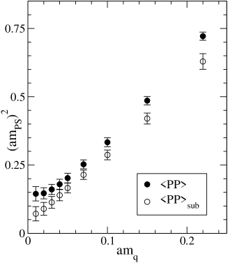
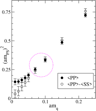
Figure 1: Effect of the subtraction of the zero modes on the pion mass (FP-ov3 operator $6^{3}\times 16$, $a=0.15~{}\mathrm{fm}$). The mass from $\langle P\,P\rangle$ is represented by filled circles, while we use open circles to represent the results from the explicit removal of the zero modes from the quark propagators (l.h.s. plot) and from the correlator $\langle PP\rangle-\langle SS\rangle$ of Eq. (3.10) (r.h.s. plot).

In this work we considered a different strategy which, from a field-theoretical point of view, is safe. There is a considerable freedom in choosing source/sink operators with given quantum numbers. This freedom can be used to cancel or reduce the topological finite size artifacts. This is the method we applied in the baryon sector, where we considered the following set of octet and decuplet operators:

$$N\, \;=\; (d^{a}{\mathcal{C}}\gamma_{5}u^{b})u^{c}\epsilon_{abc}\;,$$

$$N_{4} \;=\; (d^{a}{\mathcal{C}}\gamma_{4}\gamma_{5}u^{b})u^{c}\epsilon_{abc}\;,$$

$$\Delta\, \;=\; 2(d^{a}{\mathcal{C}}\gamma^{-}u^{b})u^{c}\epsilon_{abc}+(u^{a}{\mathcal{C}}\gamma^{-}u^{b})d^{c}\epsilon_{abc}\;,$$

$$\Delta_{4} \;=\; 2(d^{a}{\mathcal{C}}\gamma_{4}\gamma^{-}u^{b})u^{c}\epsilon_{abc}+(u^{a}{\mathcal{C}}\gamma_{4}\gamma^{-}u^{b})d^{c}\epsilon_{abc}\;.$$ (3.6)

Here ${\mathcal{C}}$ is the charge conjugation matrix, $\gamma^{-}=\gamma_{1}-i\gamma_{2}$, and the 4th direction is the time direction.

These operators can be combined in different correlators which have different quark mass singularities for their topological finite size effect. After performing the fermion contractions and isolating the zero mode contributions one finds the following leading powers for the singularities :

$$\langle\overline{N}\,N\rangle \;\sim\; (am_{q})^{-3}\;,$$ (3.7a)

$$\langle\overline{N}\,\gamma_{4}\,N\rangle \;\sim\; (am_{q})^{-2}\;,$$ (3.7b)

$$\langle\overline{N_{4}}\,N_{4}\rangle \;\sim\; (am_{q})^{-2}\;,$$ (3.7c)

$$\langle\overline{N_{4}}\,\gamma_{4}\,N_{4}\rangle \;\sim\; (am_{q})^{-1}\;.$$ (3.7d)

The first and third correlators are even, the second and fourth are odd under $t\leftrightarrow T-t$. To improve the signal we (anti)symmetrized the measured propagators. The separation of the nucleon and its negative parity partner $N^{*}$ will be addressed in Section 4. For the decuplet channel the corresponding correlators are obtained by replacing the $N$ operators by the $\Delta$ operators. The mass singularities for the different operators remain the same under this replacement.

In the meson sector the standard point-like operators are

$$P \;=\; \overline{\psi}\,\gamma_{5}\,\psi\;,$$

$$S \;=\; \overline{\psi}\,\psi\;,$$

$$A_{4} \;=\; \overline{\psi}\,\gamma_{4}\gamma_{5}\,\psi\;,$$

$$V_{i} \;=\; \overline{\psi}\,\gamma_{i}\,\psi\;.$$ (3.8)

In these expressions we suppress the flavor content of the operators and use $\psi$ for quark fields. All meson correlators we considered are flavor non-singlet. In these correlators the leading topological finite size artifacts read:

$$\langle P\,P\rangle \;\sim\; (am_{q})^{-2}\;,$$

$$\langle S\,S\rangle \;\sim\; (am_{q})^{-2}\;,$$

$$\langle A_{4}\,A_{4}\rangle \;\sim\; (am_{q})^{-1}\;,$$

$$\langle V_{i}\,V_{i}\rangle \;\sim\; (am_{q})^{-1}\;.$$ (3.9)

In Fig. 2 we show the effective mass plots for the 4 different nucleon correlators listed in Eq. (3.7) for a small (top plot) and a large quark mass (bottom plot). The data are for the $16^{3}\times 32$ lattice at $a=0.08\,\mathrm{fm}$, i.e. the lattice has a small physical volume of 1.2 fm. For the light quark (top plot) the effective mass curve from the correlator having an ${\cal O}((am_{q})^{-3})$ artifact lies significantly below those of the correlators with a reduced ${\cal O}((am_{q})^{-1})$ contribution. If the quark mass is heavy the artifact is strongly reduced and all the correlators give consistent results as the bottom plot of Fig. 2 illustrates.

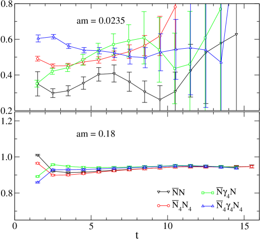
Figure 2: Effective mass plots for the nucleon measured with four different correlators $\overline{N}N$, $\overline{N}\gamma_{4}N$, $\overline{N_{4}}N_{4}$, $\overline{N_{4}}\gamma_{4}N_{4}$, on the $16^{3}\times 32$ lattice at $a=0.08\,\mathrm{fm}$ using FP. We show results for a light and a heavy quark (corresponding to $m_{\mathrm{PS}}/m_{\mathrm{V}}=0.35$ and 0.89).

For the pseudoscalar mass we followed the suggestion in [18, 52, 53] which is based on the fact that for exactly chirally symmetric actions the scalar propagator has the same topological finite size effect as the pseudoscalar propagator. Thus we can consider the difference of the pseudoscalar and scalar 2-point functions

$$\langle PP\rangle\;\;-\;\;\langle SS\rangle\;.$$ (3.10)

Since for light quarks the lightest particle in the scalar channel is much heavier than the pseudoscalar, its contribution quickly dies out with time separation. For heavy quarks, however, the relative mass difference between the pseudoscalar and scalar mass is small and a single-mass fit produces a value which is higher than the true pseudoscalar mass.

This observation suggests the following strategy: At small quark masses, where $\langle PP\rangle$ is strongly distorted, we determine the pseudoscalar mass from $\langle PP\rangle-\langle SS\rangle$. Going towards larger quark masses the effect of the zero modes is suppressed and we expect a window where the two correlators lead to consistent mass fits. In this window and beyond it we use the $\langle PP\rangle$ correlator. The r.h.s. plot in Fig. 1 illustrates [34] these expectations on a small lattice for the FP-ov3 operator. Filled symbols are used for the original $\langle PP\rangle$ correlator and open symbols for the difference $\langle PP\rangle-\langle SS\rangle$. The circle indicates the window where the zero mode effects are already negligible, but the scalar mass is much larger than the pseudoscalar and so the correct pseudoscalar mass is easily seen in the $\langle PP\rangle-\langle SS\rangle$ correlator.

For the vector meson we used the point-like vector density of Eq. (3.8) and we summed over $i=1,2,3$ in the vector meson propagator Eq. (3.9). This correlator has a remaining ${\cal O}(m_{q}^{-1})$ topological finite size effect. There exist different ways to cancel this remaining contribution also, but we neither tested nor used them in this work.

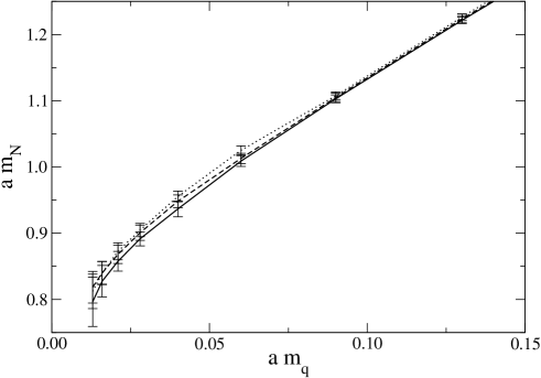
Figure 3: The dependence of the nucleon mass on the bare quark mass was measured with four different correlators. The lower and upper curves correspond to correlators (3.7a), (3.7b). The correlators (3.7c), (3.7d) give almost identical nucleon masses corresponding to the curve in the middle. FP, $16^{3}\times 32,~{}a=0.153\,\mathrm{fm}$.

Having discussed topological finite size artifacts in different operators and some strategies how to deal with them we now demonstrate that for our largest lattice with size $L=2.5$ fm they are not observed for the nucleon. We do not see such artifacts in the vector channel either.

In Fig. 3 we show the nucleon mass as a function of the quark mass (both in lattice units) determined from all 4 correlators listed in Eq. (3.7). If the topological finite size artifacts were still important for the 2.5 fm lattice then one would expect that the curves for the different operators would be different and this difference would increase substantially for small quark masses. The plots do not show such a behavior and we conclude that for the nucleon the topological finite size artifacts are negligible for $L=2.5$ fm. On the other hand, as we shall discuss in the next section, we still see a small remaining effect in the pseudoscalar sector at small quark masses even in this large volume.

4 Spectroscopy in a large volume

4.1 Discussion of the raw data

Here we present our results which were obtained in a box $L^{3}\times 2L$ with $L=2.5\,\mathrm{fm}$ for FP, $L=2.4\,\mathrm{fm}$ for CI, on a coarse lattice with $a(r_{0})=0.153\,\mathrm{fm}$ for FP and $a(r_{0})=0.148\,\mathrm{fm}$ for CI. In Section 3 we have shown that for these lattice sizes topological finite size artifacts are negligible for the baryons in the quark mass range we consider. Thus, among the different choices which we have discussed for the nucleon correlator, we here choose the most convenient one. It is a linear combination of (3.7a) and (3.7b) giving rise to a projection onto positive parity. Thus in forward time direction only the nucleon propagates and only its negative parity partner $N^{*}$ in backward time direction [55]:

$$\langle\overline{N}(0)\,\frac{1}{2}(1+\gamma_{4})\,N(t)\rangle\;\;\sim\;\;A\,\mathrm{e}^{-mt}\;+\;B\,\mathrm{e}^{-m^{*}(T-t)}\,.$$ (4.11)

For the CI operator a more detailed study of the nucleon system using a basis of three operators and a variational technique to separate ground and excited states is presented elsewhere [56].

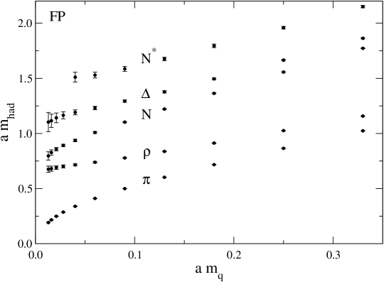
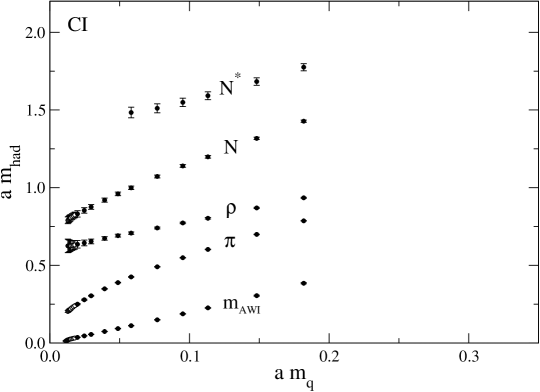
Figure 4: An overview of the hadron spectrum vs. the bare quark mass as measured with the FP action at $a=0.153\,\mathrm{fm}$ and $L=2.5\,\mathrm{fm}$. For the negative parity partner of the nucleon $N^{*}$ no reasonable mass could be obtained for the four smallest quark masses.

Figure 5: The same as Fig. 5 now for the CI action ($a=0.148\,\mathrm{fm}$ and $L=2.4\,\mathrm{fm}$).

For the vector meson the last correlator in Eq. (3.9) was used for both the FP and the CI operator. For the FP operator the pseudoscalar mass was determined from $\langle PP\rangle-\langle SS\rangle$ for small quark masses and from $\langle PP\rangle$ for larger masses as discussed in Section 3. The switching points can be found in the tables in Appendix A. For the CI operator we used the $\langle A_{4}A_{4}\rangle$ correlator.

Figures 5, 5 give an overview of our raw data on the largest volume. We plot the different hadron masses as a function of the bare quark mass for the two different Dirac operators. Although the errors increase as we approach small quark mass values, they remain under control in the $\pi,\rho,N$ and $\Delta$ channels. For the $N^{*}$ no reasonable mass and error estimate could be obtained for the smallest quark masses. The lowest data set in Fig. 5 is the axial Ward identity mass $m_{\mathrm{AWI}}$ which we will discuss in the next section.

4.2 AWI masses

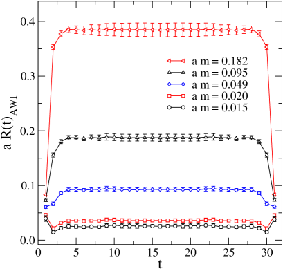
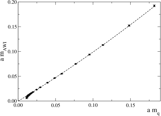
Figure 6: Time dependence of the ratio $R(t)_{\mathrm{AWI}}$ defined in Eq. (4.12) which we use to determine the axial Ward identity mass. CI, $16^{3}\times 32$, $a=0.148$ fm.

Figure 7: Bare axial Ward identity mass as a function of the bare quark mass (both in lattice units) from the CI operator on the $16^{3}\times 32$ lattice at $a=0.148$ fm. The dashed line represents a quadratic fit in $m=m_{q}+m_{\mathrm{res}}$ to the data with a few small quark masses omitted.

An important observable are quark masses from the axial Ward identity. To extract the axial Ward identity mass $m_{\mathrm{AWI}}$ we study the ratio

$$R(t)_{\mathrm{AWI}}\;\;=\;\;\frac{\langle\partial_{4}A_{4}(t)\,P(0)\rangle}{\langle P(t)\,P(0)\rangle}\;.$$ (4.12)

The axial Ward identity bare mass is then given by $a\,m_{\mathrm{AWI}}=\frac{1}{2}R(\infty)_{\mathrm{AWI}}$. In Eq. (4.12) the sink operators are projected to zero momentum and no smearing was applied to the sink. The factor from the smearing of the source operator ($P(0)$) cancels in the ratio. Note that for obtaining renormalized masses the r.h.s. of Eq. (4.12) has to be multiplied with renormalization factors; these will be discussed elsewhere [57]. Here we will use the bare values which for our purposes (fits in the pseudoscalar channel, estimate of the residual quark mass) are sufficient. Note that we use the naive current $A_{4}$ given in Eq. (3.8). The time derivative is implemented by a nearest neighbor difference.

We find that the ratio $R(t)$ exhibits excellent plateaus all the way down to our smallest quark masses. This is demonstrated in Fig. 7 where we show $R(t)$ for several quark masses. We fold the ratio around $T/2$ and subsequently fit the plateaus from $t=6\,...\,12$ to determine $am_{\mathrm{AWI}}$. The results for $a\,m_{\mathrm{AWI}}$ from the CI operator as a function of the quark mass are shown in Fig. 7. The data show essentially a linear behavior with some positive curvature at large masses. At very small quark masses we find a downward trend which is a 1-3 standard deviation effect.

In the quenched approximation the hadron propagators might contain pieces, for example contributions from topological finite size artifacts, which cannot be associated with normal contributions from energy eigenstates. In our large box these are small but can still be seen. As Tables 6, 7, 21, 22 show, the pseudoscalar mass obtained from the $\langle PP\rangle$ correlator is larger than that from $\langle PP\rangle-\langle SS\rangle$ at the smallest quark masses by 1-2 $\sigma$. The downward trend in Fig. 7 might be related to such artifacts and/or statistical fluctuations. The dashed line in this figure represents a quadratic fit in $m=m_{q}+m_{\mathrm{res}}$ to the data with the smallest quark masses omitted. Since the fit obviously does not describe the whole set of data we do not quote a value for $m_{\mathrm{res}}$.

4.3 The pseudoscalar channel

Let us now address in detail our results for the pseudoscalar mass in our largest volume. Quenched chiral perturbation theory (Q$\chi$PT) predicts [58, 59, 60]:

$$m_{\mathrm{PS}}^{2}\;=\;A\,m\;+\;B\,m\log m\;+\;C\,m^{2}\;,$$ (4.13)

where $m=m_{q}+m_{\mathrm{res}}^{\prime}$, $m_{q}$ is the bare mass of the simulation and $m_{\mathrm{res}}^{\prime}$ is an effective residual additive quark mass renormalization. As we shall discuss in the second part of this section the first two terms in (4.13) can be considered as the result of expanding the sum of the leading logarithms in the chiral log parameter $\delta$. For fixed $\delta$ and at very small quark masses this expansion is not valid anymore and the fit parameters obtained from Eq. (4.13) should be interpreted accordingly. In particular, the fit parameter $m_{\mathrm{res}}^{\prime}$ cannot be considered as a reliable prediction for the residual mass (defined as the value of $-m_{q}$ where $m_{\mathrm{PS}}$ vanishes). As shown in Figs. 8 and 9 the fit describes the data very well, yielding $m_{\mathrm{res}}^{\prime}=-0.0020(5)$(FP) and $m_{\mathrm{res}}^{\prime}=-0.002(1)$(CI).

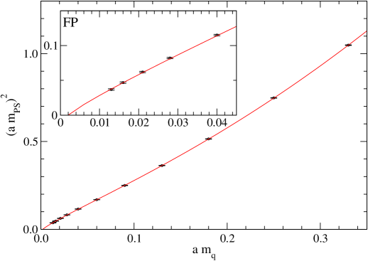
Figure 8: The square of the the pseudoscalar mass for degenerate quark masses vs. the bare quark mass (FP, $16^{3}\times 32,a=0.15$ fm). The fit is of the form suggested by Q$\chi$PT, (4.13).

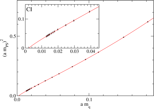
Figure 9: Same as the previous figure, now for the CI action. ($16^{3}\times 32,a=0.15$ fm). Note that the scales differ from the ones used in Fig. 8.

Note that the same fit parameters determine also the pseudoscalar masses for non-degenerate quarks [58, 60]:

$$m_{\mathrm{PS}}^{2}=A\frac{m_{1}+m_{2}}{2}\;+\;B\frac{m_{1}+m_{2}}{2}\left(\frac{m_{2}\log m_{2}-m_{1}\log m_{1}}{m_{2}-m_{1}}-1\right)\\ +C\left(\frac{m_{1}+m_{2}}{2}\right)^{2}\,.$$ (4.14)

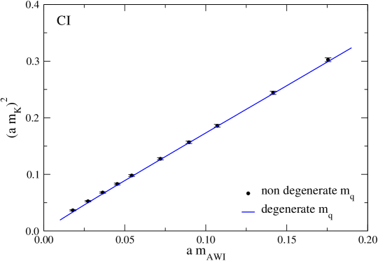
Figure 10: Comparison of pseudoscalar masses from correlators with degenerate and non-degenerate quark masses (CI, $16^{3}\times 32,a=0.15$ fm). The symbols represent the kaon mass as a function of the heavy quark mass. The full curve comes from Eq. (4.14) but the parameters $m_{\mathrm{res}}^{\prime},A,B,C$ were determined in a fit of Eq. (4.13) to data with degenerate quark masses.

We compared the measured values of $m_{\mathrm{PS}}(m_{1},m_{2})$ for the CI operator to those obtained from Eq. (4.14) (with the coefficients determined from the degenerate mass case, Eq. (4.13)). The agreement was within 1-2% and within the statistical errors. Another test is shown in Fig. 10. The data represented by the symbols were obtained from correlators with non-degenerate quark masses as follows: One quark mass (the ’heavy’) was held fixed, the other quark mass was extrapolated to the chiral limit and the procedure was repeated for different ’heavy’ quark masses. Thus the symbols essentially represent the kaon mass as a function of the $s$-quark mass. The full curve was generated from Eq. (4.14) with $m_{1}=0$ but the parameters $m_{\mathrm{res}}^{\prime}$, $A$, $B$, $C$ were determined from fitting our data with degenerate quark masses using Eq. (4.13). It is obvious that the curve falls quite well on the data points and the figure demonstrates that our degenerate and non-degenerate mass data are well compatible with each other.

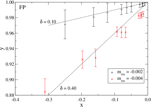
Figure 11: The plot corresponding to eqs. (4.17), (4.18) for two extreme values of the residual quark mass $m_{\mathrm{res}}$. The slope is given by the quenched parameter $\delta$ (FP, $16^{3}\times 32,a=0.15$ fm).

Let us finally comment on the quenched chiral log parameter $\delta$. Several calculations of this parameter can be found in the literature [2, 18, 19, 31, 32, 33, 34, 61, 62, 63] including also a previous result from our collaboration. These numbers range from $\delta=0.05$ to $\delta=0.23$ indicating that this is a rather difficult problem.

The $m\log m$ term in Eq. (4.13) is a quenched peculiarity which is proportional to the chiral log parameter. Nevertheless, this equation is not very useful to fix the value of $\delta$. Firstly, after expressing $B$ in terms of $\delta$ and inserting a scale parameter $\Lambda$ in the log, this equation contains too many parameters to be fitted to the data points which form a simple curve in Figs. 8, 9. Secondly, the first two terms in Eq. (4.13) are obtained from an expansion of [64]

$$m^{2}_{\mathrm{PS}}\propto m^{1/(1+\delta)}$$ (4.15)

in the parameter $\delta$. In the interesting small quark mass region the first two terms of the expansion do not give a good approximation to the function in Eq. (4.15). Thus, at least for the determination of such sensitive quantities as $m_{\mathrm{res}}$ and $\delta$, we will not use Eq. (4.13).

Trying to use Eq. (4.15) to determine $\delta$ we have to decide which points to include in the fit. Since Eq. (4.15) refers to chiral perturbation theory with degenerate quarks, we have chosen to stay below the kaon mass, i.e. $m\;<\;m_{\mathrm{s}}/2$, where $m_{\mathrm{s}}$ is the strange quark mass. In our spectroscopy with the FP operator on the coarsest lattice with large volume the lightest 5 masses satisfy this condition. The fit contains 3 parameters: amplitude, $m_{\mathrm{res}}$ and $\delta$. The results with the 4 and 5 lightest quark masses included read $m_{\mathrm{res}}=-0.0043(10)$, $\delta=0.25(7)$ and $m_{\mathrm{res}}=-0.0036(8)$, $\delta=0.19(4)$, respectively. Note that the error is statistical only. The deviation of the fit from the (correlated) data points is a small fraction of their statistical error, $\chi^{2}$ is small and gives no really useful information on the quality of the ansatz (related to the systematic error of $\delta$).

For heavy quarks we expect $m^{2}_{\mathrm{PS}}\propto m^{2}$ with a coefficient approaching 4 for very heavy quarks. The ansatz

$$m^{2}_{\mathrm{PS}}\;=\;C_{1}\,m^{1/(1+\delta)}\;+\;C_{2}\,m^{2}$$ (4.16)

describes all the data points in Figs. 8, 9 well and leads to $m_{\mathrm{res}}^{\mathrm{FP}}=-0.0027(6)$ and $\delta=0.19(1)$ in consistency with the numbers above. Again, the errors are statistical only. From these fits we quote $m_{\mathrm{res}}^{\mathrm{FP}}=-\,0.003(1)$. Note that this value is consistent with $m_{\mathrm{res}}^{\prime}$ obtained from Eq. (4.13).

Another possibility to determine $\delta$ is to start from the non-degenerate case Eq. (4.14) and to reduce the number of free parameters by forming ratios where the unknown scale $\Lambda$ and the last (quadratic) term cancel. Beyond these features the combination [2]

$$y\;=\;\frac{2m_{1}}{m_{1}+m_{2}}\;\frac{m_{\mathrm{PS},12}^{2}}{m_{\mathrm{PS},11}^{2}}\;\frac{2m_{2}}{m_{1}+m_{2}}\;\frac{m_{\mathrm{PS},12}^{2}}{m_{\mathrm{PS},22}^{2}}$$ (4.17)

is equal to 1, up to small corrections proportional to $\delta$ over our data range which justifies the expansion $y=1+\delta x+O(m^{2},\delta^{2})$, where

$$x\;=\;2\;+\;\frac{m_{1}+m_{2}}{m_{1}-m_{2}}\ln\left(\frac{m_{2}}{m_{1}}\right)\,.$$ (4.18)

With the FP we did not measure $m_{\mathrm{PS}}$ with non-degenerate quark masses needed in Eq. (4.17). However, Eq. (4.14) allows us to obtain these numbers by interpolation from measured data for the degenerate case, using the fit parameters $m_{\mathrm{res}}^{\prime}$, $A$, $B$, $C$ of Eq. (4.13). On the other hand, $m_{1}$, $m_{2}$ in Eqs. (4.17), (4.18) are the chiral mass parameters (vanishing together with $m_{\mathrm{PS}}$), with the corresponding residual quark mass $m_{\mathrm{res}}$ determined from Eqs. (4.15), (4.16). Taking $m_{\mathrm{res}}=-0.003(1)$ from above and including data only where the pseudoscalar mass is not heavier than the physical kaon mass we obtain values ranging from $\delta=0.10$ (for $m_{\mathrm{res}}=-0.002$) to $\delta=0.40$ (for $m_{\mathrm{res}}=-0.004$) as shown in Fig. 11. Obviously, this method reacts strongly to the uncertainty in the residual quark mass. The same program of different strategies to determine $\delta$ was also performed for the $CI$ operator giving similar results.

As a conclusion, we can confirm the introductory remark: The determination of the chiral log parameter is a difficult problem. It goes hand-in-hand with a reliable determination of the residual quark mass $m_{\mathrm{res}}$. In order to reduce the systematic errors one needs precise data close to the chiral limit. In light of this conclusion the error estimate in our earlier determination $\delta=0.17(2)$ for CI, $\delta=0.18(3)$ for FP [32, 33, 34] is far too optimistic.

4.4 Chiral extrapolation of vector meson and nucleon masses

We experimented with different ways of extrapolating our vector meson and nucleon data to the physical region. Firstly, we performed fits suggested by quenched chiral perturbation theory Q$\chi$PT. For vector mesons and baryons we fitted the data to the form [65, 66]:

$$m(m_{\mathrm{PS}})\;\;=\;\;m_{0}\;+\;A_{1/2}\,m_{\mathrm{PS}}\;+\;A_{1}\,m_{\mathrm{PS}}^{2}\;.$$ (4.19)

For comparison we considered the following simple fit for the vector meson (V) and baryons (B)

$$m_{\mathrm{V}}(m^{2}_{\mathrm{PS}}) \;=\; m_{0}\;+\;A_{1}\,m^{2}_{\mathrm{PS}}\;+\;A_{2}\,m^{4}_{\mathrm{PS}}\;,$$

$$m_{\mathrm{B}}^{2}(m^{2}_{\mathrm{PS}}) \;=\; m_{0}^{2}\;+\;A_{1}\,m^{2}_{\mathrm{PS}}\;+\;A_{2}\,m^{4}_{\mathrm{PS}}\;.$$ (4.20)

(The motivation for this parametrization is the observation that the dependence of $m_{\mathrm{V}}$ and $m_{\mathrm{B}}^{2}$ from $m^{2}_{\mathrm{PS}}$ is nearly linear [67].) In all cases both types of fits are good and provide a smooth inter- and extrapolation in the vector meson, nucleon, delta and negative parity nucleon channels.

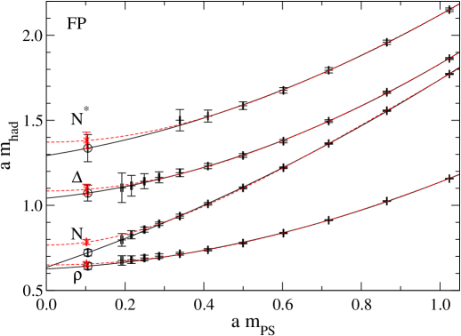
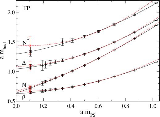
Figure 12: Chiral extrapolation of the FP data ($16^{3}\times 32,a=0.15$). We extrapolate to the point where $m_{\pi}/m_{\rho}$ takes its physical value (open circle). Two different fits are compared here: the one suggested by Q$\chi$PT theory (4.19) (solid lines) and an ad-hoc form with powers of $m_{\mathrm{PS}}^{2}$ (4.4) (dashed lines). All quantities are measured in lattice units.

Figure 13: Chiral extrapolation for FP ($16^{3}\times 32,a=0.15$), similar to Fig. 13. Both fits are of the form (4.19), but in one of them (dashed line) the two heaviest quark masses are not included.

Although the form of Eq. (4.19) is suggested by Q$\chi$PT we use it here beyond the range of its validity, i.e. as an effective parametrization. In Fig. 13 we give a graphical view of the fits, of their extrapolation and of the physical mass prediction in lattice units for the FP action. The full curves were fitted with the Q$\chi$PT formula from Eq. (4.19) while the dashed curves correspond to the ad-hoc form of Eq. (4.4). The extrapolated nucleon mass differs by more than 2 $\sigma$ for these two extrapolations, while the shifts in the other channels are small.

Although the fits using the ansatz from Q$\chi$PT seem to be excellent, the way we used it above does not take the theoretical background of this ansatz seriously: It was applied for the whole range of our quark masses, although some of them are obviously outside the validity of Q$\chi$PT. Thus in order to estimate this systematic error we experimented also with reducing the fit region for the bare quark masses and analyzed the effect on the extrapolated hadron masses. Fig. 13 illustrates the effect of excluding the two largest quark masses from the fit on the extrapolated mass values for the FP operator. We find that the effect is less than 1 $\sigma$ in all the channels.

For the CI operator we also performed a series of fits experimenting with both the Q$\chi$PT formula (4.19) and the ansatz (4.4). In our fits we also varied the number of large quark mass data taken into account and the degree of the polynomials in (4.19), (4.4). Similarly to the FP operator we found that the variation of the extrapolated masses is a 1 $\sigma$ effect for the vector meson and the negative parity nucleon and slightly larger (1.5 $\sigma$) for the nucleon. In Fig. 14 we show the two extremal fits which are given by Q$\chi$PT (4.19) with all masses (full curve) and the ansatz (4.4) with all masses (dashed curve).

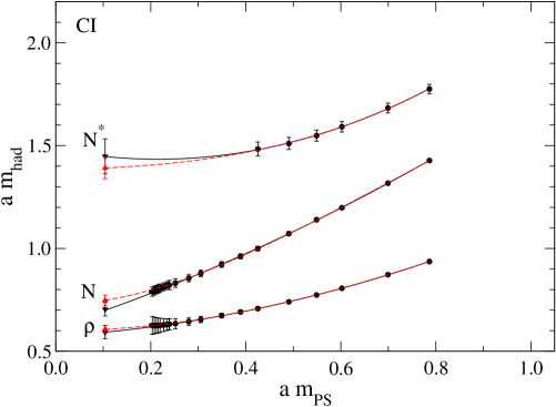
Figure 14: Chiral extrapolation for the CI operator ($16^{3}\times 32,a=0.15$). We show the Q$\chi$PT fit (4.19) using solid lines and the fit to (4.4) with dotted lines. All quantities are measured in lattice units.

4.5 Setting the scale - results in physical units

Three parameters enter light hadron spectroscopy: the lattice spacing $a$, the average mass of the light quarks $m_{\mathrm{ud}}=(m_{u}+m_{d})/2$ and the strange quark mass $m_{\mathrm{s}}$. In order to determine their values, one has to identify observables measured on the lattice with experimental values in the continuum. However, as the quenched spectrum does not coincide with the physical one, the determination of the parameters is ambiguous. As is well known, depending on the choice of experimental data to fit the parameters the quenching errors in the prediction can be shifted around. Nevertheless, we want to argue below that the quenching errors show an intuitively understandable pattern in hadron spectroscopy and the spectrum has more consistency than it is usually believed to have. Similar observations were made earlier in [37]. Here we compare three different procedures to set the physical input:

• The masses $m_{\pi},m_{\rho}$ and $m_{K}$ or $m_{\Phi}$ are used as experimental input data. The scale $a(\rho)$ is set using the $\rho$ mass. To determine the light quark mass the pseudoscalar and vector masses are extrapolated to that value $m_{\mathrm{ud}}$, where the physical value of $m_{\pi}/m_{\rho}$ is reached. To determine the strange quark mass, we either use the $K$ or the $\Phi$ mass as input. This is a widely used procedure.

• The Sommer parameter $r_{0}$ (=0.5 fm) and the masses $m_{\pi}$ and $m_{K}$, or $m_{\pi}$ and $m_{\Phi}$ are used as experimental input data. The scale $a(r_{0})$ is set from the Sommer parameter. To determine the light quark mass the pseudoscalar mass was extrapolated to the value $m_{\mathrm{ud}}$, where the physical value of $r_{0}m_{\pi}$ is reached. To determine the strange quark mass, we again either use the $K$ or the $\Phi$ mass as input.
  

• The masses $m_{\pi},m_{K}$ and $m_{\Phi}$ are used as experimental input data. The scale $a(\Phi)$ is set by requiring $m_{\mathrm{V}}(m_{\mathrm{s}})=m_{\Phi}$. The values $m_{\mathrm{s}}$ and $m_{\mathrm{ud}}$ are obtained from the ratios $m_{\mathrm{PS}}(m_{\mathrm{s}},m_{\mathrm{ud}})/m_{\mathrm{V}}(m_{\mathrm{s}})=m_{K}/m_{\Phi}$ and $m_{\mathrm{PS}}(m_{\mathrm{ud}})/m_{\mathrm{V}}(m_{\mathrm{s}})=m_{\pi}/m_{\Phi}$.

	$a_{\mathrm{FP}}$	$a_{\mathrm{CI}}$
$\rho$	$0.165(5)\,\mathrm{fm}$	$0.154(8)~{}\mathrm{fm}$
$r_{0}$	$0.153(2)\,\mathrm{fm}$	$0.148(2)~{}\mathrm{fm}$
$\Phi$	$0.1536(14)\,\mathrm{fm}$	$0.146(2)~{}\mathrm{fm}$

Table 2: The lattice constant extracted from the $\rho$, the $r_{0}$ and the $\Phi$ scale (methods I, II and III). The errors quoted are the statistical ones.

Before discussing the results, let us have a look at the sources of systematic errors. In method I the scale is set by an extrapolated value of the vector meson mass. The systematic error of these extrapolations is discussed in the previous Section 4.4. Also the statistical error in the vector channel is increasing rapidly with decreasing quark mass. Concerning method II one has to remark that also the determination of $r_{0}$ is plagued by uncertainties. Firstly, the physical value of the Sommer parameter is not known precisely and, secondly, its extraction becomes more difficult on coarse lattices. Method III seems to be better protected from such systematic problems.

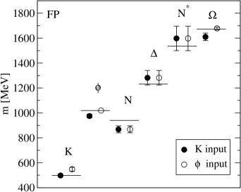
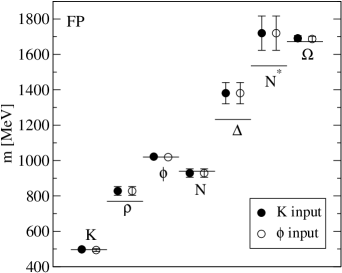
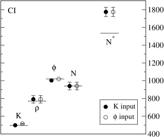
Figure 15: The prediction for the hadron masses using the conventional way to fix the parameters (method I): The lattice spacing $a(\rho)$ and the light quark mass are fixed by $m_{\pi}$ and $m_{\rho}$, while the strange quark mass is taken from $m_{K}$ or $m_{\phi}$. The l.h.s. plot shows the FP results, the CI data can be found on the r.h.s. The horizontal lines indicate the experimental numbers.

Figure 16: The hadron masses with the lattice spacing $a(r_{0})$ taken from the Sommer parameter. The light and strange quark masses are fixed using $m_{\pi}$ and $m_{K}$ or $m_{\rho}$ (method II).

Figure 17: Here the lattice spacing $a(\Phi)$, the light and strange quark masses are fixed by $m_{\pi}$, $m_{K}$ and $m_{\Phi}$ (method III). The Sommer parameter is a prediction in this case: $r_{0}=0.49(1)$ fm for both FP and CI.

The results for the spectrum obtained with these three procedures are presented in Figs. 16, 16 and Fig. 17. The l.h.s. plots give the FP data, while the r.h.s. plots show the results from CI. The errors shown are only statistical errors and were estimated by jackknife resampling: All the necessary steps (finding the fit parameters to the data, solving equations, etc.) were repeated on every jackknife sample. Our results for the scales are collected in Table 2. Again the errors given are only the statistical ones.

Let us now discuss the merits and problems of the different methods. Using method I (Fig. 16 and Table 5) we find the well-known qualitative features of this standard approach. (The fit parameters are: FP: $a=0.165(5)\,{\rm fm}$, $am_{\rm ud}=0.0033(2)$, $am_{\rm s}=0.113(7)$[K-input], $am_{\rm s}=0.139(17)$[$\Phi$-input]; CI: $a=0.154(8)~{}\mathrm{fm}$, $am_{\rm s}=0.093(6)$[K-input], $am_{\rm s}=0.115(12)$[$\Phi$-input].) The predictions for the masses of hadrons containing strange quarks depend rather strongly on using the $K$ or the $\Phi$ meson mass as an input. The scale, set by the $\rho$ in this method, lies higher than that obtained in the gauge sector by $r_{0}$. (Although, as Table 2 shows, for CI all the three scales are compatible within the statistical errors.)

Setting the scale by $r_{0}$ (method II, Fig. 16 and Table 5 ) the discrepancy between the spectra with $m_{K}$ vs. $m_{\Phi}$ input disappears. Even more, these masses and the $\Omega$ are shifted to their right place. Since they have small statistical errors this is a non-trivial coincidence. (The parameters are: FP: $a=a(r_{0})=0.153\,{\rm fm}$, $am_{\rm ud}=0.0027(1)$, $am_{\rm s}=0.0954(13)$[K-input], $am_{\rm s}=0.0939(35)$[$\Phi$-input]; CI: $a=a(r_{0})=0.148(2)\,{\rm fm}$, $am_{\rm s}=0.083(1)$[K-input], $am_{\rm s}=0.090(3)$[$\Phi$-input].)

From the consistency of the $m_{K}$ vs. $m_{\Phi}$ input above it follows that method III (Fig. 17 and Table 5) predicts essentially the same spectrum as method II. In this case the $r_{0}$ is a prediction. We obtain $r_{0}=0.49(1)\,\mathrm{fm}$ for both FP and CI. (Fit parameters: FP: $a=0.1536(14)\,{\rm fm}$, $am_{\rm ud}=0.0028(1)$, $am_{\rm s}=0.0962(22)$; CI: $a=0.146(2)~{}\mathrm{fm}$, $am_{\rm s}=0.078(27)$.)

We note at this point that unlike the quenched $\delta$ parameter, the hadron spectrum is quite insensitive to the actual choice of $m_{\mathrm{res}}^{\prime}$. Indeed $m_{\mathrm{res}}^{\prime}$ enters our analysis only through the use of Eq. (4.14) in the determination of $m_{K}$. But even taking the extreme value of $m_{\mathrm{res}}^{\prime}=0$, the hadron masses change only by a fraction of their statistical errors while $a$ changes by $1\,\sigma$ (1%) and $am_{\rm ud}$, $am_{\rm s}$ are changed by 15% and 8%, respectively.

The hadron spectrum in Figs. 16 and 17 shows a feature which is easy to understand intuitively: Quenched spectroscopy works fine for the narrow $K$ (or $\Phi$), $N$ and $\Omega$, while it has problems with the broad resonances $\rho,\Delta$ and $N^{*}$ with widths $\approx$150, 120 and 150 MeV, respectively. It would be interesting to test this intuitive picture on other resonances, in particular on baryons with non-degenerate quarks which were not treated in our analysis.

Hadron	Exp.	K-input		$\Phi$-input
		FP	CI	FP	CI
K	0.498	—	—	0.548(16)	0.547(16)
$\Phi$	1.019	0.975(15)	0.970(25)	—	—
N	0.940	0.868(28)	0.965(46)	0.868(28)	0.965(46)
$\Delta$	1.232	1.282(59)	—	1.282(59)	—
$N^{*}$	1.535	1.598(98)	1.745(59)	1.598(98)	1.745(59)
$\Omega$	1.673	1.610(30)	—	1.678(11)	—

Table 3: Hadron masses in GeV with the scale and quark masses set by $\pi$-$\rho$-K and $\pi$-$\rho$-$\Phi$ input (method I).

Hadron	Exp.	K-input		$\Phi$-input
		FP	CI	FP	CI
K	0.498	—	—	0.494(8)	0.515(4)
$\rho$	0.768	0.828(25)	0.791(42)	0.828(25)	0.791(42)
$\Phi$	1.019	1.022(6)	1.003(8)	—	—
N	0.940	0.928(24)	0.940(43)	0.928(24)	0.940(43)
$\Delta$	1.232	1.381(60)	—	1.381(60)	—
$N^{*}$	1.535	1.720(97)	1.775(52)	1.720(97)	1.775(52)
$\Omega$	1.673	1.691(15)	—	1.687(15)	—

Table 4: Hadron masses in GeV when the scale is set using the Sommer parameter $r_{0}=0.5~{}{\rm fm}$ (method II).

Hadron	Exp.	FP	CI
$\rho$	0.768	0.824(20)	0.812(43)
N	0.940	0.925(24)	0.978(44)
$\Delta$	1.232	1.375(60)	—
$N^{*}$	1.535	1.714(98)	1.824(53)
$\Omega$	1.673	1.686(14)	—

Table 5: Hadron masses in GeV with the scale $a$ and the quark masses fixed by the $\pi,K,\Phi$ masses (method III).

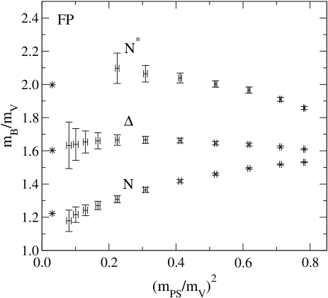
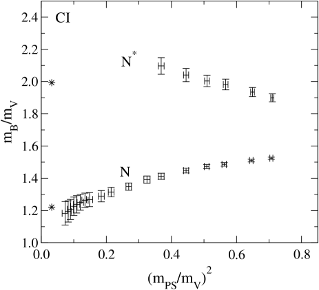
Figure 18: APE plot for $N$, $\Delta$ and $N^{*}$ in the FP case ($16^{3}\times 32,a=0.15$ fm). The asterisks indicate the experimental numbers.

Figure 19: APE plot for $N$ and $N^{*}$ from the CI operator ($16^{3}\times 32,a=0.15$ fm).

To complete our presentation of hadron spectroscopy in a large volume we present standard APE plots in Figs. 19 and 19, where the mass ratios $m_{N}/m_{\mathrm{V}}$, $m_{\Delta}/m_{\mathrm{V}}$, $m_{N^{*}}/m_{\mathrm{V}}$ are plotted against $(m_{\mathrm{PS}}/m_{\mathrm{V}})^{2}$ for the FP action and the same for the CI action (without the $\Delta$).

5 Volume dependence and scaling properties

The results of our large volume spectroscopy discussed in the previous section were obtained on a rather coarse $a=0.15\,\mathrm{fm}$ lattice. It is, therefore, essential to check the size of cut-off effects. In this section we shall also compare our results with those of recent large scale simulations. Similarly, we want to see, whether our $L=2.5\,\mathrm{fm}$ lattice used for spectroscopy is sufficiently large to neglect physical finite size effects. In full QCD the pion cloud around the hadrons would dominate the finite size effects in such a large box. In the quenched approximation this is expected to be strongly suppressed. Indeed, the finite size effects were found to be significantly smaller in quenched QCD than in full QCD [54]. The authors of [68] found no finite size effects for $L>2\,\mathrm{fm}$ on the 2% level. In [54] a $6\pm 3$% decrease was observed in the nucleon mass in $L=(1.6-2.4)\,\mathrm{fm}$ (see also [3] and the summary in [69]). For the vector meson the corrections are smaller. Although the situation is not completely coherent, the earlier results suggest that the finite size effects in our $L=2.5\,\mathrm{fm}$ box should be small. However, since our pions are light we explicitly checked for finite size effects.

We tried to plan our simulations carefully, but we made errors nevertheless. Mentioning them here might help others to avoid them. A large part of the scaling test was done in a fixed small $L=1.2\,\mathrm{fm}$ volume and the number of configurations was chosen to be approximately the same as in the large volume simulations. The fluctuations in the small volume are, however, stronger which makes our scaling tests less stringent. In addition, we were running with the same quark mass set on the small volume (scaling test) as on the large volume (spectroscopy). This made little sense since the scaling test is most interesting for the heavy, compact objects, while most of the computer time was spent on the light objects.

5.1 Scaling tests

The parameters of our simulation allow us to compare spectroscopic data in a fixed $L=1.2\,\mathrm{fm}$ volume at three different resolutions (see Table 1): $a(r_{0})=0.153\,\mathrm{fm}$, $0.102\,\mathrm{fm}$, $0.077\,\mathrm{fm}$ and $a(r_{0})=0.148\,\mathrm{fm}$, $0.102\,\mathrm{fm}$, $0.078\,\mathrm{fm}$ for the FP and CI actions, respectively.

As discussed in Section 3, the topological finite size artifacts are large in such a small volume at small quark masses. This is the case not only for the pion, but also for the nucleon as has been illustrated in Fig. 2. Here it is mandatory to use correlators for which these artifacts are suppressed.

Our statistics in this small volume simulation is poorer than in the large volume spectroscopy. For reasons discussed in Section 2.3 we decided to use uncorrelated fits with the weight $\mathrm{Cov}_{\mathrm{measd}}$ in (2.4) for the FP operator while we continued to use correlated fits for the CI case. In the Appendix we collect the pseudoscalar, vector and nucleon mass predictions for different quark masses. In a few cases at small quark masses, our statistics and the difficulty with the zero mode artifacts did not allow us to get a mass prediction with a reliable error estimate. No numbers are quoted in these cases.

Fig. 21 shows the dependence of the vector meson and the nucleon mass on the lattice resolution for different quark masses. The hadron masses are measured in $m_{\mathrm{V}}(x_{0}),x_{0}=0.75$ units, i.e. in terms of the mass of the vector meson at $m_{\mathrm{PS}}/m_{\mathrm{V}}=0.75$. For large quark masses the hadrons are expected to be more compact and so more sensitive to the lattice resolution. Within the errors, the nucleon channel shows no cut-off effects neither for large nor for small quark masses. We used appropriate correlators to reduce/cancel the quenched zero mode artifacts. The strange behavior in the vector channel at small quark masses for $a=0.08\,\mathrm{fm}$ might be related to the remaining ${\cal O}((am_{q})^{-1})$ zero mode effects. It should be noted that for the vector meson curve the (0.75,1.0) point is fixed independently of $a$ which makes this case less informative for testing scaling violations. Furthermore, considering mass ratios might cancel parts of the cut-off effects in general. Fig. 21 is the equivalent plot for the CI action and similarly to the FP case the data for the different values of $a$ are compatible within error bars.

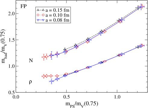
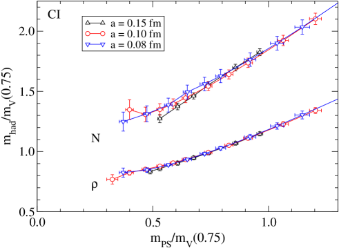
Figure 20: Scaling test in a small volume of $L=1.2\,\mathrm{fm}$ for vector meson (lower curve) and the nucleon at three values of the lattice spacing. The hadron masses are measured in $m_{\mathrm{V}}(x_{0}),x_{0}=0.75$ units, i.e. in terms of the mass in the vector meson channel at $m_{\mathrm{PS}}/m_{\mathrm{V}}=0.75$. We used correlators with reduced quenched zero mode artifacts. The strange behavior in the vector channel at small quark masses on the finest lattice might be related to the remaining ${\cal O}((am_{q})^{-1})$ zero mode effects.

Figure 21: Same as Fig. 21 for the CI operator. The standard nucleon correlator was used here.

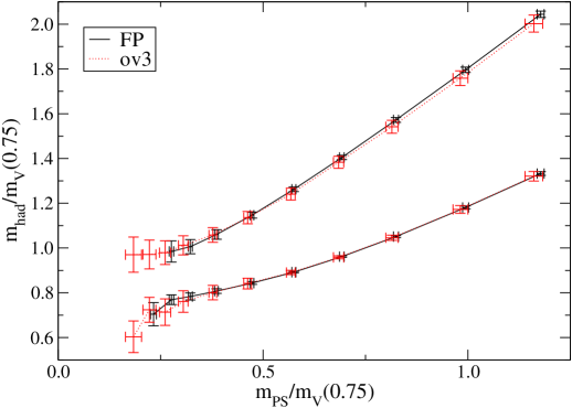
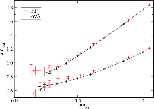
Figure 22: Results obtained with two different Dirac operators (FP and FP+3 overlap steps) are compared here at fixed $a(r_{0})=0.153\,\mathrm{fm}$ in a box of $L=1.8\,\mathrm{fm}$. The nucleon (upper curve) and vector meson masses are measured in $m_{\mathrm{V}}(x=0.75)$ units like in Fig. 21.

Figure 23: The same as Fig. 23 but in terms of the dimensionless hadron masses. This is a correct comparison since they were measured on the same gauge configurations in this quenched study.

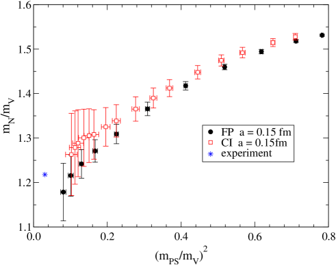
Figure 24: The APE plots for the nucleon with the FP and CI actions.

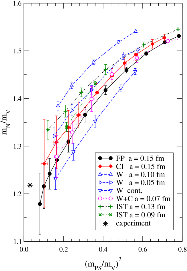
Figure 25: The APE plots for the nucleon with the FP and CI actions are compared to those obtained by CP-PACS at $a=0.10\,\mathrm{fm}$, $a=0.05\,\mathrm{fm}$ and their continuum extrapolation, by MILC at $a=0.13\,\mathrm{fm}$, $a=0.09\,\mathrm{fm}$ and with clover improved Wilson fermions at $a=0.07$ fm. The asterisk indicates the experimental number.

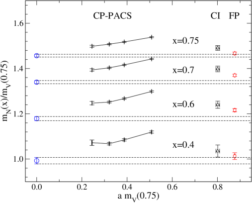
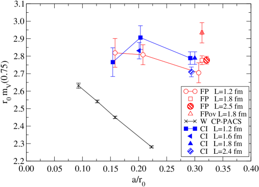
Figure 26: The nucleon mass $m_{\mathrm{N}}(x)$ interpolated to $m_{\mathrm{PS}}/m_{\mathrm{V}}=x$ vs. the lattice spacing at four different values of $x$, in units of $m_{\mathrm{V}}(0.75)$. For the Wilson action the four data points and their continuum extrapolations (open circles) are taken from [2](CP-PACS). The values with the FP action are on the right at $am_{\mathrm{V}}(0.75)\approx 0.87$ ($a=0.153\,\mathrm{fm}$), the CI data ($a=0.148\,\mathrm{fm}$) slightly left of the FP numbers.

Figure 27: The scaling behavior of $r_{0}m_{\mathrm{V}}(x=0.75)$. Since no finite volume effects were observed in $m_{\mathrm{V}}$ in the region $L=1.2-2.5\,\mathrm{fm}$ (see Fig. 29) we included data from different volumes in this figure. Results from four different actions are compared here: FP, FP+3 overlap steps (1 data point only), CI and Wilson fermions from CP-PACS.

Figs. 23 and 23 compare the results from two different Dirac operators: the parametrized FP and the one obtained from this after 3 overlap projection steps. The latter has smaller deviations from a GW solution, but might be driven away from the fixed-point of the renormalization group transformation used to construct the FP action. Fig. 23 compares the vector and nucleon masses in $m_{\mathrm{V}}(x_{0}),x_{0}=0.75$ units at $a(r_{0})=0.153\,\mathrm{fm}$ in a box of size $L=1.8\,\mathrm{fm}$. No difference can be seen within the errors. Since the gauge configurations are the same for the two Dirac operators (i.e. $a(r_{0})$ is fixed and the same) we can compare the dimensionless hadron masses $am_{h}$ directly. In this way we avoid taking mass ratios which might cancel part of the cut-off effects. The corresponding Fig. 23 indicates some deviations beyond the statistical error in the vector channel for larger quark masses. This might be a (small) cut-off effect coming from one (or both) of the Dirac operators, but Fig. 23 does not reveal which Dirac operator is responsible for it.

Figs. 24 and 25 are APE plots where the large volume FP and CI results (Fig. 24) and the FP, CI, CP-PACS [2], improved staggered MILC [31, 10] and clover improved Wilson results [67] (Fig. 25) are compared. The continuum extrapolation of the CP-PACS data is also given in Fig. 25. This non-trivial continuum extrapolation is illustrated in Fig. 27, where the FP and CI numbers are repeated again. We can draw the following conclusions from these figures. The FP and CI APE-plots are consistent with each other. The improved staggered results at $a=0.13\,\mathrm{fm}$ and $a=0.09\,\mathrm{fm}$ are lying above the FP curve beyond the statistical errors. If we assume that the CP-PACS continuum extrapolation is correct then the FP results at $a=0.15\,\mathrm{fm}$ show cut-off effects, but they are closer to the continuum than the Wilson results at $a=0.05\,\mathrm{fm}$ and the improved staggered results at $a=0.13\,\mathrm{fm}$ and $a=0.09\,\mathrm{fm}$.

Finally, we connect the hadronic observables with the Sommer parameter $r_{0}$ obtained in the gauge sector. Fig. 27 shows $r_{0}m_{\mathrm{V}}(x=0.75)$ as a function of $a/r_{0}$. This figure compares data for three different resolutions at fixed $L=1.2\,\mathrm{fm}$. As we shall see in the next section we observe no finite size effects in the vector meson channel in the region $L=1.2-2.5\,\mathrm{fm}$. For this reason we included in this figure data from different volumes also.

The FP and CI data obtained in a fixed $L=1.2\,\mathrm{fm}$ box show no cut-off effects beyond the errors and are consistent with each other. The same conclusion can be drawn if we include points obtained at larger volumes. On the other hand, the prediction of the Dirac operator after 3 overlap steps at $a(r_{0})=0.153\,\mathrm{fm}$ in a box $L=1.8\,\mathrm{fm}$ deviates from that of the FP operator on the same lattice (this was already shown by Fig. 23). For comparison, the CP-PACS Wilson action results [2] for $a=0.05-0.1\,\mathrm{fm}$ are also given.

5.2 Finite size effects

We studied the spectrum in three different volumes $L=2.5\,\mathrm{fm}$, $L=1.8\,\mathrm{fm}$ and $L=1.2\,\mathrm{fm}$ at fixed lattice unit $a~{}=0.15~{}\mathrm{fm}$. Figs. 29 and 29 show the volume dependence of the N, V and PS masses as a function of the quark mass. No finite size effects are seen beyond the errors, except for the nucleon in the smallest $L=1.2\,\mathrm{fm}$ box. In this small box the nucleon mass is pushed upwards as the quark mass is decreased.

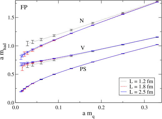
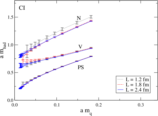
Figure 28: Hadron masses in the PS, V and N channels vs. the bare quark mass, measured with the FP action at $a=0.15\,\mathrm{fm}$ and at three different lattice volumes. The nucleon mass shows finite size effects at $L=1.2\,\mathrm{fm}$, while the PS and V meson data indicate no finite size effects even in such a small lattice volume in our quenched simulation.

Figure 29: Same as Fig. 29, now for the CI operator.

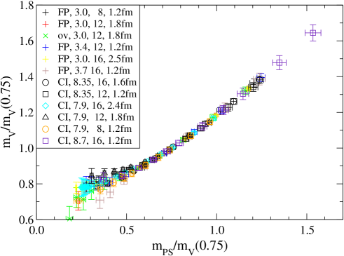
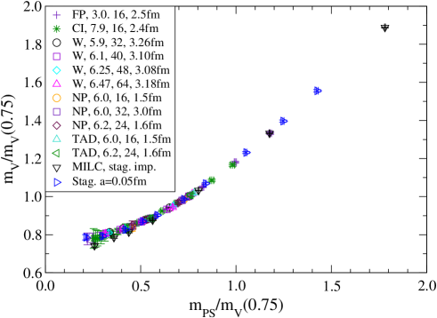
Figure 30: The masses $m_{\mathrm{V}}$ vs. $m_{\mathrm{PS}}$, both in $m_{\mathrm{V}}(0.75)$ units. We show all our results for the FP and CI operators.

Figure 31: The masses $m_{\mathrm{V}}$ vs. $m_{\mathrm{PS}}$, both in $m_{\mathrm{V}}(0.75)$ units. The Wilson data (W) are taken from [2], the nonperturbatively improved (NP) and tadpole improved (TAD) data from [3], the staggered improved data (MILC) from [31], and the staggered data from [61]. In the legend we indicate the $\beta$ values of the corresponding gauge action, the spatial lattice size in lattice units and in fm.

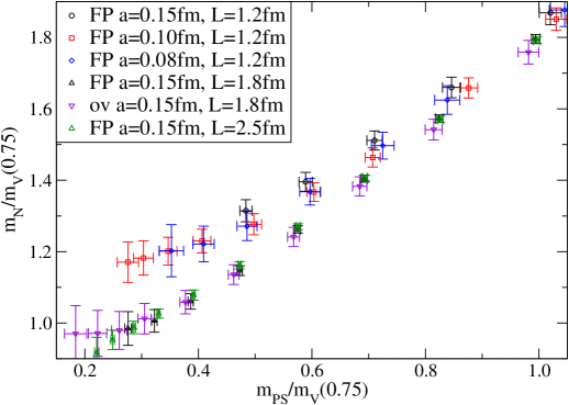
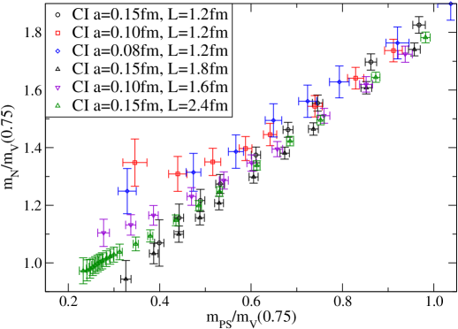
Figure 32: The nucleon mass vs. the pseudoscalar mass, both measured in $m_{\mathrm{V}}(0.75)$ units for the FP action at different lattice spacings and physical volumes. The small-volume data at $L=1.2\,\mathrm{fm}$ show scaling. The three volumes at $a=0.15\,\mathrm{fm}$ shows finite size effects at $L=1.2\,\mathrm{fm}$, but not for $L\geq 1.8\,\mathrm{fm}$.

Figure 33: Same as Fig. 33 now for the CI operator.

Figs. 31 and 31 show data in different volumes and lattice resolutions for the vector meson and the nucleon mass as a function of the pseudoscalar mass, where all the masses are measured in $m_{\mathrm{V}}(0.75)$ units. The somewhat unexpected message from Fig. 31 is that the vector meson mass in these units is largely independent of the cut-off, of the volume and of the action used, i.e. the cut-off effects are practically absorbed by $m_{\mathrm{V}}(0.75)$.

Fig. 33 summarizes what we already saw in earlier figures of the nucleon mass from the FP action. The points referring to a fixed $L=1.2\,\mathrm{fm}$ box at three different resolutions run together, no cut-off effects are seen. On the other hand, in this smallest box the nucleon shows significant finite size effects which are decreasing as the quark mass is increasing. There is no finite size effect seen when comparing the $L=1.8\,\mathrm{fm}$ and $L=2.5\,\mathrm{fm}$ results. At heavy quark masses all the points join to form a single curve indicating the absence both of finite size and cut-off effects.

In the case of the CI operator the interpretation of the corresponding Fig. 33 is similar, although the separation into two sets of data, one suffering from finite size effects, one free of them is not as clear-cut as for the FP operator. The main reason is that for the CI medium size volumes the physical size is slightly different. We have $L=1.6$ fm and $L=1.8$ for our $16^{3}\times 32,\beta=8.35$, respectively $12^{3}\times 24,\beta=7.90$ CI lattices. For the FP operator the two corresponding lattices both have the somewhat larger size $L=1.8$. Fig. 33 shows that the $L=1.6$ fm data lie in between the $L=1.2$ results clearly suffering from finite size effects and the $L=1.8$ fm and $L=2.4$ fm data essentially free of them. The drop of the $L=1.8$ fm data below the $L=2.4$ fm results at small quark masses is probably due to the topological finite size artifacts (we did not use improved operators here). We remark that in [56] where a linear combination of three nucleon operators was used, this discrepancy is resolved.

Acknowledgements: The calculations were done on the Hitachi SR8000 at the Leibniz Rechenzentrum in Munich and at the Swiss Center for Scientific Computing in Manno. We thank the LRZ and CSCS staff for training and support. This work was supported in parts by DFG, BMBF, SNF, the European Community’s Human Potential Programme under contract HPRN-CT-2000-00145, the DOE under grant DOE-FG03-97ER40546 and the Fonds zur Förderung der Wissenschaftlichen Forschung in Österreich, project FWF-P16310-N08. C. Gattringer acknowledges support by the Austrian Academy of Sciences (APART 654). The authors thank Gunnar Bali, Gilberto Colangelo, Christine Davies, Tom DeGrand, Anna Hasenfratz, Rainer Sommer and Stewart Wright for useful discussions.

Appendix A Data obtained with the FP action

We list here the measured hadron masses for different input bare quark masses. All the masses are in lattice units. The numbers in brackets give the jackknife errors. We give also the value of $\chi^{2}_{\mathrm{df}}$ of the fit and the fit range. In cases where we could not use a correlated fit with the measured covariance matrix (see, Section 2.3), the value of $\chi^{2}_{\mathrm{df}}$ does not characterize the quality of the fit. In these cases no $\chi^{2}_{\mathrm{df}}$ is quoted.

The pseudoscalar mass was determined from the $\langle PP\rangle-\langle SS\rangle$ and the $\langle PP\rangle$ correlators for small and large quark masses, respectively (see Section 3). The corresponding switching-point (the quark mass at and above which the $\langle PP\rangle$ correlator is used) is quoted in the table caption. In a few cases (mainly in small volumes at small quark masses) we did not quote the hadron mass since the error was very large and difficult to pin down.

We measured the baryon spectrum using several different correlators (see Section 3). In most of the cases (in particular in large volumes) the correlator in (3.7a) proved to be the best choice for the nucleon and and the analogous one for $\Delta$. The exceptions are indicated in the table caption.

$16^{3}\times 32$, $\beta=3.0$, parametrized FP
$am_{q}$	$am_{\rm PS}$(P)	$\chi^{2}_{df}$	$t$	$am_{\rm PS}$(P-S)	$\chi^{2}_{df}$	$t$	$am_{\rm V}$	$t$
0.013	0.1992(31)	1.5	[6,13]	0.1919(30)	0.9	[6,16]	0.676(28)	[5,10]
0.016	0.2227(20)	1.1	[6,16]	0.2163(24)	0.9	[6,14]	0.681(23)	[5,10]
0.021	0.2535(15)	0.9	[6,16]	0.2489(20)	0.8	[6,14]	0.691(16)	[5,9]
0.028	0.2891(14)	0.7	[6,16]	0.2865(17)	0.7	[6,13]	0.701(13)	[5,10]
0.04	0.3401(13)	0.5	[6,16]	0.3393(15)	0.5	[6,16]	0.716(9)	[5,9]
0.06	0.4107(12)	0.5	[6,16]	0.4118(14)	0.4	[6,16]	0.739(7)	[6,9]
0.09	0.4997(11)	0.5	[6,16]	0.5023(13)	0.6	[7,16]	0.778(5)	[6,10]
0.13	0.6024(11)	0.6	[6,16]	0.6049(13)	1.0	[8,16]	0.837(3)	[6,10]
0.18	0.7173(10)	0.8	[6,16]	0.7196(12)	1.6	[9,16]	0.913(3)	[7,12]
0.25	0.8650(9)	0.8	[6,16]	0.8665(12)	1.7	[11,16]	1.025(2)	[7,12]
0.33	1.0240(9)	0.6	[6,16]	1.0257(11)	1.1	[11,16]	1.158(2)	[7,12]

Table 6: Pseudo-scalar and vector meson masses on a $16^{3}\times 32$ lattice at $\beta=3.0$ with $D^{\rm FP}$. The switching-point is $am_{q}=0.06$.

$16^{3}\times 32$, $\beta=3.0$, parametrized FP
$am_{q}$	$am_{\rm Oct}$(N)	$\chi^{2}_{df}$	$t$	$am_{\rm Dec}(\Delta)$	$t$	$am_{\rm Oct}$ $(N^{*})$	$t$
0.013	0.797(37)	0.4	[5,7]	1.104(87)	[5,8]
0.016	0.828(24)	0.2	[5,7]	1.115(61)	[5,8]
0.021	0.858(15)	0.7	[5,8]	1.142(44)	[5,8]
0.028	0.892(11)	1.1	[5,10]	1.165(32)	[5,8]
0.04	0.937(12)	1.1	[7,12]	1.192(22)	[5,8]	1.511(45)	[4,6]
0.06	1.009(8)	1.3	[7,16]	1.231(15)	[5,8]	1.530(27)	[4,6]
0.09	1.103(6)	0.4	[7,16]	1.293(11)	[5,8]	1.586(23)	[4,6]
0.13	1.222(5)	0.2	[7,14]	1.377(10)	[6,9]	1.676(16)	[4,6]
0.18	1.364(4)	0.4	[7,14]	1.495(8)	[6,9]	1.795(16)	[4,8]
0.25	1.557(4)	0.6	[7,14]	1.665(7)	[6,9]	1.959(13)	[4,8]
0.33	1.772(4)	0.7	[7,14]	1.863(6)	[6,9]	2.150(11)	[4,8]

Table 7: The masses of the nucleon $N$, the $\Delta$ and the negative parity partner of the nucleon $N^{*}$ on a $16^{3}\times 32$ lattice at $\beta=3.0$ with $D^{\rm FP}$.

$12^{3}\times 24$, $\beta=3.0$, parametrized FP
$am_{q}$	$am_{\rm PS}$(P)	$t$	$am_{\rm PS}$(P-S)	$t$	$am_{\rm V}$	$t$
0.016	0.2484(144)	[6,12]	0.2019(63)	[5,12]	0.612(46)	[6,10]
0.021	0.2621(40)	[5,12]	0.2399(46)	[5,12]	0.668(20)	[5,10]
0.028	0.2941(31)	[5,12]	0.2801(38)	[5,12]	0.681(16)	[5,10]
0.04	0.3428(25)	[5,12]	0.3356(30)	[5,12]	0.701(11)	[5,10]
0.06	0.4108(23)	[5,10]	0.4108(23)	[5,12]	0.732(8)	[5,10]
0.09	0.4994(20)	[6,10]	0.5029(19)	[6,12]	0.775(6)	[5,12]
0.13	0.6013(17)	[6,10]	0.6075(15)	[6,12]	0.835(4)	[5,12]
0.18	0.7159(15)	[6,10]	0.7235(14)	[7,12]	0.913(3)	[6,12]
0.25	0.8636(13)	[6,10]	0.8717(12)	[7,12]	1.026(2)	[6,12]
0.33	1.0227(12)	[6,10]	1.0307(11)	[7,12]	1.158(2)	[6,12]

Table 8: Pseudo-scalar and vector meson masses on a $12^{3}\times 24$ lattice at $\beta=3.0$ with $D^{\rm FP}$. The switching-point is $am_{q}=0.06$.

$12^{3}\times 24$, $\beta=3.0$, parametrized FP
$am_{q}$	$am_{\rm Oct}$(N)	$t$	$am_{\rm Dec}(\Delta)$	$t$	$am_{\rm Oct}(N^{*})$	$t$
0.016
0.021	0.855(41)	[6, 9]
0.028	0.874(27)	[6, 9]	0.984(69)	[6,10]
0.04	0.921(18)	[6,10]	1.016(67)	[7,10]
0.06	0.996(11)	[6,10]	1.146(43)	[7,10]
0.09	1.096(7)	[6,10]	1.264(25)	[7,10]
0.13	1.220(5)	[6,10]	1.374(14)	[7,10]
0.18	1.366(4)	[6,12]	1.497(9)	[7,10]	1.738(33)	[6,10]
0.25	1.560(3)	[6,12]	1.667(7)	[7,10]	1.927(23)	[6,10]
0.33	1.776(3)	[6,12]	1.862(6)	[7,12]	2.131(18)	[6,10]

Table 9: The masses of the nucleon $N$, the $\Delta$ and the negative parity partner of the nucleon $N^{*}$ on a $12^{3}\times 24$ lattice at $\beta=3.0$ with $D^{\rm FP}$. For the nucleon at $am_{q}=0.021$ and 0.028 the correlator Eq. (3.7d) was used.

$12^{3}\times 24$, $\beta=3.0$, parametrized FP + 3 overlap steps
$am_{q}$	$am_{\rm PS}$(P)	$t$	$am_{\rm PS}$(P-S)	$t$	$am_{\rm V}$	$t$
0.009			0.133(24)	[6, 9]
0.012			0.169(18)	[6, 9]	0.554(69)	[6, 9]
0.016	0.2301(83)	[6,10]	0.204(15)	[6, 9]	0.664(56)	[6, 8]
0.021	0.2605(70)	[6,10]	0.239(12)	[6, 9]	0.655(60)	[6,10]
0.028	0.2981(59)	[6,10]	0.280(10)	[6, 9]	0.698(51)	[6,10]
0.04	0.3528(48)	[6,10]	0.3462(71)	[6,10]	0.735(37)	[6,10]
0.06	0.4278(39)	[6,10]	0.4243(51)	[6,10]	0.772(31)	[6,12]
0.09	0.5210(31)	[6,10]	0.5213(37)	[6,10]	0.818(19)	[6,12]
0.13	0.6280(26)	[6,10]	0.6319(31)	[6,10]	0.879(11)	[6,12]
0.18	0.7476(22)	[6,10]	0.7545(27)	[6,10]	0.960(8)	[6,12]
0.25	0.9008(20)	[6,10]	0.9116(21)	[6,12]	1.076(6)	[6,12]
0.33	1.0652(19)	[6,10]	1.0757(21)	[6,12]	1.212(5)	[6,12]

Table 10: Pseudo-scalar and vector meson masses on a $12^{3}\times 24$ lattice at $\beta=3.0$ with $D^{\rm FP}$+ 3 overlap steps. The switching-point is $am_{q}=0.09$.

$12^{3}\times 24$, $\beta=3.0$, parametrized FP   +3 overlap steps
$am_{q}$	$am_{\rm Oct}$(N)	$t$	$am_{\rm Dec}(\Delta)$	$t$
0.009	0.897(81)	[4, 6]	0.87(15)	[4, 6]
0.012	0.890(65)	[4, 6]	0.92(10)	[4, 6]
0.016	0.891(52)	[4, 6]	1.004(79)	[4, 6]
0.021	0.899(43)	[4, 7]	1.071(76)	[4, 7]
0.028	0.929(34)	[4, 8]	1.134(70)	[4, 7]
0.04	0.971(24)	[4, 8]	1.191(60)	[4, 7]
0.06	1.042(16)	[4, 8]	1.256(48)	[4, 8]
0.09	1.139(14)	[5, 8]	1.336(44)	[5, 9]
0.13	1.269(12)	[5, 9]	1.434(31)	[5,10]
0.18	1.415(10)	[5, 9]	1.560(22)	[5,10]
0.25	1.614(9)	[5, 9]	1.738(16)	[5,10]
0.33	1.838(9)	[5, 9]	1.944(14)	[5,10]

Table 11: The masses of the nucleon $N$ and the $\Delta$ on a $12^{3}\times 24$ lattice at $\beta=3.0$ with $D^{\rm FP}$ + 3 overlap steps. For the nucleon and $\Delta$ the operator in Eq. (3.7c) was used.

$12^{3}\times 24$, $\beta=3.4$, parametrized FP
$am_{q}$	$am_{\rm PS}$(P)	$t$	$am_{\rm PS}$(P-S)	$t$	$am_{\rm V}$	$t$
0.029	0.193(10)	[7,10]	0.161(11)	[7,12]	0.470(23)	[7,9]
0.032	0.201(9)	[7,12]	0.177(10)	[7,12]	0.474(18)	[7,9]
0.037	0.218(7)	[7,12]	0.202(8)	[7,12]	0.468(19)	[7,10]
0.045	0.247(6)	[7,12]	0.237(8)	[8,12]	0.475(17)	[8,12]
0.058	0.292(4)	[7,12]	0.291(6)	[8,12]	0.498(11)	[8,12]
0.078	0.352(4)	[8,12]	0.356(5)	[9,12]	0.528(9)	[9,12]
0.10	0.413(3)	[8,12]	0.419(4)	[9,12]	0.566(7)	[9,12]
0.14	0.511(3)	[8,12]	0.520(3)	[9,12]	0.637(5)	[9,12]
0.18	0.601(2)	[8,12]	0.611(3)	[9,12]	0.708(4)	[9,12]
0.24	0.727(2)	[8,12]	0.738(2)	[9,12]	0.814(3)	[9,12]

Table 12: Pseudo-scalar and vector meson masses on a $12^{3}\times 24$ lattice at $\beta=3.4$ with $D^{\rm FP}$. The switching-point is $am_{q}=0.078$.

$12^{3}\times 24$, $\beta=3.4$, parametrized FP
$am_{q}$	$am_{\rm Oct}$(N)	$t$	$am_{\rm Dec}(\Delta)$	$t$	$am_{\rm Oct}$ $(N^{*})$	$t$
0.029	0.683(32)	[6, 9]	0.720(92)	[7,12]
0.032	0.690(27)	[6, 9]	0.748(64)	[7,10]
0.037	0.701(21)	[6, 9]	0.769(52)	[7,10]
0.045	0.718(17)	[6,10]	0.794(50)	[7,12]
0.058	0.745(15)	[6,12]	0.835(35)	[7,12]	1.088(56)	[5,8]
0.078	0.798(10)	[6,12]	0.890(23)	[7,12]	1.103(24)	[5,8]
0.10	0.854(10)	[8,12]	0.949(16)	[7,12]	1.135(20)	[6,8]
0.14	0.968(7)	[8,12]	1.048(12)	[8,12]	1.238(13)	[6,8]
0.18	1.080(6)	[8,12]	1.151(9)	[8,12]	1.344(10)	[6,8]
0.24	1.247(5)	[8,12]	1.305(7)	[8,12]	1.503(8)	[6,8]

Table 13: The masses of the nucleon $N$, the $\Delta$ and the negative parity partner of the nucleon $N^{*}$ on a $12^{3}\times 24$ lattice at $\beta=3.4$ with $D^{\rm FP}$. For the nucleon the correlator Eq. (3.7c) has been used.

$16^{3}\times 32$, $\beta=3.7$, parametrized FP
$am_{q}$	$am_{\rm PS}$(P)	$t$	$am_{\rm PS}$(P-S)	$t$	$am_{\rm V}$	$t$
0.0235	0.126(13)	[10,13]	0.123(18)	[10,13]
0.026	0.139(11)	[10,13]	0.141(13)	[10,13]
0.03	0.157(9)	[10,13]	0.163(10)	[10,13]	0.316(23)	[10,16]
0.036	0.182(7)	[10,13]	0.190(8)	[10,13]	0.336(18)	[10,16]
0.045	0.216(6)	[10,13]	0.227(6)	[10,16]	0.363(14)	[10,16]
0.06	0.266(4)	[10,13]	0.275(5)	[10,16]	0.398(10)	[10,16]
0.08	0.323(3)	[10,16]	0.330(5)	[12,16]	0.437(7)	[10,16]
0.1	0.373(3)	[10,16]	0.380(4)	[12,16]	0.474(5)	[10,16]
0.14	0.466(2)	[10,16]	0.471(3)	[12,16]	0.546(4)	[10,16]
0.18	0.551(2)	[10,16]	0.555(3)	[12,16]	0.618(3)	[10,16]

Table 14: Pseudo-scalar and vector meson masses on a $16^{3}\times 32$ lattice at $\beta=3.7$ with $D^{\rm FP}$. The switching-point is $am_{q}=0.026$.

$16^{3}\times 32$, $\beta=3.7$, parametrized FP
$am_{q}$	$am_{\rm Oct}$(N)	$t$
0.0235	0.515(86)	[8,11]
0.026	0.530(51)	[8,11]
0.03	0.536(29)	[8,11]
0.036	0.544(19)	[8,11]
0.045	0.566(14)	[8,11]
0.06	0.609(12)	[8,11]
0.08	0.667(10)	[8,11]
0.1	0.724(9)	[8,11]
0.14	0.836(8)	[8,11]
0.18	0.947(7)	[8,11]

Table 15: The masses of the nucleon $N$ on a $16^{3}\times 32$ lattice at $\beta=3.7$ with $D^{\rm FP}$. The correlator Eq. (3.7d) has been chosen here.

$8^{3}\times 24$, $\beta=3.0$, parametrized FP
$am_{q}$	$am_{\rm PS}$(P)	$t$	$am_{\rm V}$	$t$
0.028			0.652(34)	[5, 9]
0.04			0.670(28)	[5,10]
0.06	0.409(6)	[5,10]	0.701(21)	[5,10]
0.09	0.498(5)	[5,10]	0.754(15)	[5,10]
0.13	0.601(4)	[5,10]	0.822(11)	[5,10]
0.18	0.716(4)	[5,10]	0.905(8)	[5,10]
0.25	0.863(3)	[5,10]	1.021(6)	[5,10]
0.33	1.022(3)	[5,10]	1.153(4)	[5,10]

Table 16: Pseudo-scalar and vector meson masses on a $8^{3}\times 24$ lattice at $\beta=3.0$ with $D^{\rm FP}$. We found it difficult to obtain controlled mass predictions in the $P-S$ channel on that lattice with our statistics. We do not give numbers for this channel.

$8^{3}\times 24$, $\beta=3.0$, parametrized FP
$am_{q}$	$am_{\rm Oct}$(N)	$t$
0.028	1.042(40)	[4, 7]
0.04	1.070(29)	[4, 7]
0.06	1.112(21)	[4, 8]
0.09	1.181(16)	[4, 8]
0.13	1.279(13)	[4, 9]
0.18	1.404(11)	[4, 9]
0.25	1.581(9)	[4, 9]
0.33	1.785(8)	[4, 9]

Table 17: The masses of the nucleon $N$ on a $8^{3}\times 24$ lattice at $\beta=3.0$ with $D^{\rm FP}$. For the nucleon the correlator in Eq. (3.7d) was used.

$16^{3}\times 32$, $\beta=3.0$, parametrized FP
$x$	$m_{\mathrm{N}}(x)/m_{\mathrm{V}}(x)$	$m_{\Delta}(x)/m_{\mathrm{V}}(x)$
0.40	1.258(22)	1.644(44)
0.45	1.294(16)	1.651(34)
0.50	1.329(13)	1.658(28)
0.55	1.365(11)	1.666(24)
0.60	1.399(9)	1.669(20)
0.65	1.427(7)	1.665(15)
0.70	1.453(6)	1.658(11)
0.75	1.476(5)	1.646(9)
0.80	1.498(5)	1.633(9)

Table 18: Mass ratios interpolated to $m_{\mathrm{PS}}/m_{\mathrm{V}}=x$ on a $16^{3}\times 32$ lattice at $\beta=3.0$ with $D^{\mathrm{FP}}$.

$16^{3}\times 32$, $\beta=3.0$, parametrized FP
$am_{q}$	$m_{\mathrm{PS}}/m_{\mathrm{V}}$	$m_{\mathrm{N}}/m_{\mathrm{V}}$	$m_{\Delta}/m_{\mathrm{V}}$	$m_{\mathrm{N}^{*}}/m_{\mathrm{V}}$
0.013	0.284(13)	1.179(65)	1.633(140)
0.016	0.318(11)	1.216(47)	1.639(96)
0.021	0.361(9)	1.242(32)	1.654(66)
0.028	0.408(8)	1.271(25)	1.661(49)
0.04	0.474(6)	1.309(22)	1.665(31)	2.111(66)
0.06	0.556(5)	1.366(15)	1.666(22)	2.071(40)
0.09	0.642(4)	1.418(9)	1.662(14)	2.039(30)
0.13	0.720(3)	1.460(6)	1.646(11)	2.003(20)
0.18	0.786(2)	1.494(5)	1.638(9)	1.966(18)
0.25	0.844(2)	1.518(3)	1.624(6)	1.910(12)
0.33	0.885(1)	1.531(3)	1.610(5)	1.858(9)

Table 19: Mass ratios on a $16^{3}\times 32$ lattice at $\beta=3.0$ with $D^{\mathrm{FP}}$.

$16^{3}\times 32$, $\beta=3.0$, parametrized FP
$x$	$m_{\mathrm{V}}(x)/m_{\mathrm{V}}(x_{0})$	$m_{\mathrm{N}}(x)/m_{\mathrm{V}}(x_{0})$	$m_{\Delta}(x)/m_{\mathrm{V}}(x_{0})$
0.40	0.794(14)	1.013(15)	1.324(32)
0.45	0.810(12)	1.058(12)	1.350(28)
0.50	0.829(10)	1.106(11)	1.379(24)
0.55	0.850(8)	1.158(9)	1.413(20)
0.60	0.875(6)	1.216(7)	1.452(17)
0.65	0.907(4)	1.286(6)	1.501(13)
0.70	0.947(2)	1.370(5)	1.563(11)
0.75	1.00	1.476(5)	1.646(9)
0.80	1.076(3)	1.614(6)	1.760(8)

Table 20: Hadron masses interpolated to $m_{\mathrm{PS}}/m_{\mathrm{V}}=x$ in units of $m_{\mathrm{V}}(x_{0})$ with $x_{0}=0.75$ on a $16^{3}\times 32$ lattice at $\beta=3.0$ with $D^{\mathrm{FP}}$.

Appendix B Data obtained with the CI action

In this appendix the extracted masses for the CI operator are presented. The techniques used and the quantities computed are the same as in the case of the FP operator. However, there are a few differences: For the PS mass we list the results for the $\langle A_{4}A_{4}\rangle$ correlator as well which we used in the figures and in the fits to the data. Only in Tables 33 and 34 we use the combination of $\langle PP\rangle-\langle SS\rangle$ and the $\langle PP\rangle$ results for the pseudo-scalar mass. There the switching point is at $am_{q}=0.04$. We use Eq. (4.11) to extract the nucleon and $N^{*}$ mass.

$16^{3}\times 32$, $\beta=7.9$, CI
$am_{q}$	$am_{\mathrm{PS}}$(P)	$\chi^{2}_{\mathrm{df}}$	$t$	$am_{\mathrm{PS}}$(A)	$\chi^{2}_{\mathrm{df}}$	$t$	$am_{\mathrm{PS}}$(P-S)	$\chi^{2}_{\mathrm{df}}$	$t$
0.0129	0.2074(39)	0.6	[7,14]	0.2031(61)	1.1	[7,12]	0.2002(56)	2.9	[6,12]
0.0134	0.2120(36)	0.6	[7,14]	0.2076(60)	1.2	[7,12]	0.2051(55)	2.9	[6,12]
0.0139	0.2163(33)	0.6	[7,14]	0.2117(59)	1.4	[7,12]	0.2095(54)	3.0	[6,12]
0.0144	0.2204(31)	0.6	[7,14]	0.2157(58)	1.5	[7,12]	0.2137(53)	3.0	[6,12]
0.0149	0.2242(30)	0.6	[7,14]	0.2195(56)	1.6	[7,12]	0.2176(52)	3.0	[6,12]
0.0159	0.2315(28)	0.6	[7,14]	0.2268(54)	1.8	[7,12]	0.2251(49)	3.0	[6,12]
0.0169	0.2384(26)	0.7	[7,14]	0.2336(52)	1.9	[7,12]	0.2323(46)	3.0	[6,12]
0.0178	0.2450(25)	0.7	[7,14]	0.2402(50)	2.0	[7,12]	0.2392(43)	3.0	[6,12]
0.0198	0.2572(24)	0.6	[7,16]	0.2502(37)	1.8	[7,16]	0.2526(38)	2.9	[6,12]
0.0247	0.2850(22)	0.8	[7,16]	0.2786(32)	1.9	[7,16]	0.2808(36)	2.5	[8,16]
0.0296	0.3099(21)	1.0	[7,16]	0.3040(29)	1.9	[7,16]	0.3073(33)	2.3	[8,16]
0.0392	0.3544(19)	1.1	[7,16]	0.3490(25)	1.8	[7,16]	0.3541(28)	2.1	[8,16]
0.0488	0.3937(18)	1.1	[7,16]	0.3889(22)	1.7	[7,16]	0.3950(25)	1.9	[8,16]
0.0583	0.4295(17)	1.1	[7,16]	0.4254(21)	1.6	[7,16]	0.4318(22)	1.7	[8,16]
0.0769	0.4939(16)	0.9	[7,16]	0.4907(19)	1.4	[7,16]	0.4972(19)	1.2	[8,16]
0.0952	0.5515(15)	0.8	[7,16]	0.5490(18)	1.2	[7,16]	0.5554(17)	0.8	[8,16]
0.1132	0.6045(14)	0.7	[7,16]	0.6024(18)	1.1	[7,16]	0.6086(16)	0.5	[8,16]
0.1482	0.7006(14)	0.6	[7,16]	0.6992(17)	1.0	[7,16]	0.7048(15)	0.4	[8,16]
0.1818	0.7875(14)	0.7	[7,16]	0.7865(17)	0.9	[7,16]	0.7917(16)	0.5	[8,16]

Table 21: Results for the meson correlators for the CI Dirac operator at $\beta_{1}=7.90$ on the $16^{3}\times 32$ lattice.

$16^{3}\times 32$, $\beta=7.90$, CI
$am_{q}$	$am_{\mathrm{V}}$	$\chi^{2}_{\mathrm{df}}$	$t$	$am_{\mathrm{N}}$	$\chi^{2}_{\mathrm{df}}$	$t$	$am_{\mathrm{N^{*}}}$	$\chi^{2}_{\mathrm{df}}$	$t$
0.0129	0.625(44)	1.4	[6,9]	0.790(22)	0.2	[4,8]
0.0134	0.625(41)	1.4	[6,9]	0.795(21)	0.2	[4,8]
0.0139	0.625(38)	1.4	[6,9]	0.799(21)	0.3	[4,8]
0.0144	0.625(36)	1.3	[6,9]	0.803(20)	0.4	[4,8]
0.0149	0.626(34)	1.3	[6,9]	0.807(20)	0.5	[4,8]
0.0159	0.628(31)	1.3	[6,9]	0.813(19)	0.7	[4,8]
0.0169	0.629(29)	1.2	[6,9]	0.819(19)	0.8	[4,8]
0.0178	0.631(27)	1.1	[6,9]	0.824(19)	0.9	[4,8]
0.0198	0.635(24)	1.1	[6,9]	0.831(21)	1.4	[5,8]
0.0247	0.644(19)	0.6	[6,11]	0.854(18)	1.6	[5,8]
0.0296	0.654(15)	0.4	[6,11]	0.876(15)	0.8	[5,12]
0.0392	0.673(11)	0.2	[6,11]	0.919(13)	0.7	[5,12]
0.0488	0.6909(93)	0.1	[6,11]	0.960(12)	0.5	[5,12]	1.480(40)	2.0	[3,6]
0.0583	0.7075(79)	0.1	[6,11]	0.999(11)	0.4	[5,12]	1.484(34)	1.4	[3,6]
0.0769	0.7404(61)	0.2	[6,11]	1.0720(96)	0.5	[5,12]	1.511(29)	0.7	[3,6]
0.0952	0.7729(52)	1.7	[6,12]	1.1396(87)	0.6	[5,12]	1.549(27)	0.4	[3,6]
0.1132	0.8031(48)	1.9	[7,12]	1.1983(85)	0.4	[6,12]	1.592(26)	0.4	[3,6]
0.1482	0.8696(38)	1.8	[7,12]	1.3171(77)	0.6	[6,12]	1.683(24)	0.5	[3,6]
0.1818	0.9346(33)	1.5	[7,12]	1.4278(72)	0.6	[6,12]	1.775(23)	0.6	[3,6]

Table 22: Results for the vector meson and the nucleon for the CI Dirac operator at $\beta=7.90$ on the $16^{3}\times 32$ lattice.

$12^{3}\times 24$, $\beta=7.90$, CI
$am_{q}$	$am_{\mathrm{PS}}$(P)	$\chi^{2}_{\mathrm{df}}$	t	$am_{\mathrm{AA}}$(P)	$\chi^{2}_{\mathrm{df}}$	$t$	$am_{\mathrm{PS}}$(P-S)	$\chi^{2}_{\mathrm{df}}$	$t$
0.020	0.2560(64)	1.2	[7,12]	0.2688(86)	0.7	[6,12]	0.2527(66)	0.8	[6,12]
0.030	0.3107(47)	0.8	[7,12]	0.3191(67)	0.6	[6,12]	0.3112(49)	1.0	[6,12]
0.040	0.3561(40)	0.6	[7,12]	0.3642(65)	0.5	[7,12]	0.3510(58)	0.7	[8,12]
0.049	0.3960(36)	0.5	[7,12]	0.4023(58)	0.3	[7,12]	0.3922(52)	0.9	[8,12]
0.058	0.4321(33)	0.5	[7,12]	0.4370(52)	0.2	[7,12]	0.4293(47)	1.0	[8,12]
0.077	0.4967(30)	0.4	[7,12]	0.4993(45)	0.4	[7,12]	0.4954(41)	1.1	[8,12]
0.095	0.5543(28)	0.4	[7,12]	0.5552(41)	0.7	[7,12]	0.5544(36)	1.0	[8,12]
0.113	0.6073(27)	0.4	[7,12]	0.6072(38)	1.0	[7,12]	0.6084(33)	0.9	[8,12]
0.148	0.7033(25)	0.4	[7,12]	0.7025(33)	1.2	[7,12]	0.7059(30)	1.0	[8,12]
0.182	0.7902(24)	0.5	[7,12]	0.7892(30)	1.1	[7,12]	0.7934(29)	1.2	[8,12]

Table 23: Results for the pseudoscalar correlators for the CI Dirac operator at $\beta=7.90$ on the $12^{3}\times 24$ lattice.

$12^{3}\times 24$, $\beta=7.90$, CI
$am_{q}$	$am_{\mathrm{V}}$	$\chi^{2}_{\mathrm{df}}$	$t$	$am_{\mathrm{N}}$	$\chi^{2}_{\mathrm{df}}$	$t$
0.020	0.696(37)	1.2	[6,11]	0.778(53)	0.1	[5,9]
0.030	0.709(24)	1.7	[6,11]	0.851(28)	0.5	[5,10]
0.040	0.716(18)	2.1	[6,11]	0.906(21)	0.8	[5,10]
0.049	0.724(14)	2.2	[6,11]	0.954(17)	1.2	[5,10]
0.058	0.734(12)	2.0	[6,11]	0.996(15)	0.9	[5,12]
0.077	0.7584(89)	1.6	[6,11]	1.070(12)	0.9	[5,12]
0.095	0.7865(71)	1.3	[6,11]	1.138(11)	0.9	[5,12]
0.113	0.8170(60)	0.9	[6,12]	1.207(12)	1.1	[6,12]
0.148	0.8792(47)	0.7	[6,12]	1.325(10)	1.5	[6,12]
0.182	0.9413(41)	0.6	[6,12]	1.4351(96)	1.8	[6,12]

Table 24: Results for the vector meson and the nucleon for the CI Dirac operator at $\beta=7.90$ on the $12^{3}\times 24$ lattice.

$8^{3}\times 24$, $\beta=7.90$, CI
$am_{q}$	$am_{\mathrm{PS}}$(P)	$\chi^{2}_{\mathrm{df}}$	$t$	$am_{\mathrm{PS}}$(A)	$\chi^{2}_{\mathrm{df}}$	$t$	$am_{\mathrm{PS}}$(P-S)	$\chi^{2}_{\mathrm{df}}$	$t$
0.020	0.308(20)	0.2	[7,12]	0.282(12)	0.6	[6,11]	0.192(23)	0.0	[6,11]
0.030	0.325(11)	0.9	[7,12]	0.329(10)	1.0	[6,11]	0.293(11)	1.9	[6,11]
0.040	0.3651(90)	0.9	[7,12]	0.365(10)	0.7	[7,11]	0.353(12)	1.9	[8,11]
0.049	0.4026(80)	0.8	[7,12]	0.4034(93)	0.6	[7,11]	0.396(10)	1.9	[8,11]
0.058	0.4373(74)	0.7	[7,12]	0.4389(88)	0.5	[7,11]	0.4348(93)	1.9	[8,11]
0.077	0.5006(65)	0.6	[7,12]	0.5034(80)	0.6	[7,11]	0.5020(80)	1.9	[8,11]
0.095	0.5577(59)	0.6	[7,12]	0.5614(75)	0.6	[7,11]	0.5612(70)	1.8	[8,11]
0.113	0.6104(54)	0.5	[7,12]	0.6146(70)	0.7	[7,11]	0.6151(64)	1.7	[8,11]
0.148	0.7064(48)	0.4	[7,12]	0.7109(62)	0.7	[7,11]	0.7125(55)	1.4	[8,11]
0.182	0.7935(43)	0.4	[7,12]	0.7977(56)	0.7	[7,11]	0.8002(50)	1.2	[8,11]

Table 25: Results for the meson correlators for the CI Dirac operator at $\beta=7.90$ on the $8^{3}\times 24$ lattice.

$8^{3}\times 24$, $\beta=7.90$, CI
$am_{q}$	$am_{\mathrm{V}}$	$\chi^{2}_{\mathrm{df}}$	$t$	$am_{\mathrm{N}}$	$\chi^{2}_{\mathrm{df}}$	$t$
0.020	0.581(47)	0.3	[6,9]
0.030	0.634(29)	0.0	[6,9]	0.88(11)	0.1	[5,9]
0.040	0.665(24)	0.0	[6,9]	0.954(60)	0.2	[5,10]
0.049	0.688(21)	0.1	[6,9]	1.003(45)	0.1	[5,10]
0.058	0.708(19)	0.1	[6,9]	1.050(37)	0.1	[5,10]
0.077	0.745(15)	0.1	[6,10]	1.133(28)	0.3	[5,10]
0.095	0.781(13)	0.1	[6,10]	1.206(25)	0.5	[5,10]
0.113	0.816(12)	0.1	[6,10]	1.282(27)	0.6	[6,10]
0.148	0.8814(94)	0.1	[6,12]	1.399(25)	0.9	[6,10]
0.182	0.9461(82)	0.2	[6,12]	1.505(24)	1.2	[6,10]

Table 26: Results for the vector meson and the nucleon for the CI Dirac operator at $\beta=7.90$ on the $8^{3}\times 24$ lattice.

$16^{3}\times 32$, $\beta=8.35$, CI
$am_{q}$	$am_{\mathrm{PS}}$(P)	$\chi^{2}_{\mathrm{df}}$	$t$	$am_{\mathrm{PS}}$(A)	$\chi^{2}_{\mathrm{df}}$	$t$	$am_{\mathrm{PS}}$(P-S)	$\chi^{2}_{\mathrm{df}}$	$t$
0.010	0.1734(40)	0.7	[7,16]	0.1757(58)	1.8	[6,16]	0.1599(74)	0.9	[8,16]
0.015	0.2015(29)	0.9	[7,16]	0.2043(46)	1.9	[6,16]	0.1941(61)	0.8	[8,16]
0.020	0.2268(25)	1.0	[7,16]	0.2294(41)	2.0	[6,16]	0.2226(52)	0.8	[8,16]
0.030	0.2712(21)	1.2	[7,16]	0.2731(34)	1.8	[6,16]	0.2704(41)	0.8	[8,16]
0.039	0.3099(19)	1.3	[7,16]	0.3113(30)	1.6	[6,16]	0.3112(34)	0.9	[8,16]
0.049	0.3448(18)	1.3	[7,16]	0.3460(27)	1.5	[6,16]	0.3462(32)	1.1	[9,16]
0.058	0.3770(17)	1.4	[7,16]	0.3780(24)	1.3	[6,16]	0.3795(28)	1.3	[9,16]
0.077	0.4356(16)	1.4	[7,16]	0.4363(21)	1.1	[6,16]	0.4394(23)	1.5	[9,16]
0.095	0.4887(16)	1.3	[7,16]	0.4893(19)	1.0	[6,16]	0.4932(20)	1.6	[9,16]
0.113	0.5380(15)	1.3	[7,16]	0.5385(18)	1.0	[6,16]	0.5430(19)	1.6	[9,16]
0.148	0.6286(15)	1.2	[7,16]	0.6290(17)	1.1	[6,16]	0.6340(17)	1.6	[9,16]
0.182	0.7117(14)	1.1	[7,16]	0.7120(16)	1.2	[6,16]	0.7171(17)	1.6	[9,16]

Table 27: Results for the meson correlators for the CI Dirac operator at $\beta=8.35$ on the $16^{3}\times 32$ lattice.

$16^{3}\times 32$, $\beta=8.35$, CI
$am_{q}$	$am_{\mathrm{V}}$	$\chi^{2}_{\mathrm{df}}$	$t$	$am_{\mathrm{N}}$	$\chi^{2}_{\mathrm{df}}$	$t$
0.010	0.450(21)	0.4	[7,12]	0.636(25)	2.0	[4,11]
0.015	0.452(15)	0.4	[7,12]	0.652(17)	2.1	[4,11]
0.020	0.460(12)	0.4	[7,12]	0.674(14)	2.0	[4,11]
0.030	0.4813(88)	0.4	[7,12]	0.708(13)	1.8	[5,13]
0.039	0.5019(71)	0.6	[7,12]	0.746(12)	1.8	[5,13]
0.049	0.5217(60)	0.9	[7,12]	0.775(11)	1.9	[6,13]
0.058	0.5410(54)	1.2	[7,12]	0.810(10)	2.0	[6,13]
0.077	0.5790(45)	1.6	[7,12]	0.8699(88)	1.8	[7,14]
0.095	0.6164(39)	1.8	[7,12]	0.9326(79)	1.8	[7,14]
0.113	0.6533(35)	1.8	[7,12]	0.9931(73)	1.8	[7,14]
0.148	0.7254(30)	1.8	[7,12]	1.1094(65)	1.7	[7,14]
0.182	0.7950(27)	1.8	[7,12]	1.2202(60)	1.6	[7,14]

Table 28: Results for the vector meson and the nucleon for the CI Dirac operator at $\beta=8.35$ on the $16^{3}\times 32$ lattice.

$12^{3}\times 24$, $\beta=8.35$, CI
$am_{q}$	$am_{\mathrm{PS}}$(P)	$\chi^{2}_{\mathrm{df}}$	$t$	$am_{\mathrm{PS}}$(A)	$\chi^{2}_{\mathrm{df}}$	$t$	$am_{\mathrm{PS}}$(P-S)	$\chi^{2}_{\mathrm{df}}$	$t$
0.010	0.185(14)	0.9	[7,12]	0.169(17)	1.8	[6,12]	0.120(27)	2.1	[8,12]
0.020	0.2287(95)	1.6	[7,12]	0.227(11)	1.6	[6,12]	0.204(16)	1.4	[8,12]
0.030	0.2708(72)	1.6	[7,12]	0.2684(89)	1.2	[6,12]	0.260(11)	0.7	[8,12]
0.039	0.3089(60)	1.5	[7,12]	0.3055(76)	1.0	[6,12]	0.3050(92)	0.5	[8,12]
0.049	0.3437(53)	1.4	[7,12]	0.3396(67)	1.0	[6,12]	0.3411(89)	0.5	[9,12]
0.058	0.3758(49)	1.4	[7,12]	0.3713(62)	1.1	[6,12]	0.3765(78)	0.5	[9,12]
0.077	0.4344(45)	1.3	[7,12]	0.4296(55)	1.4	[6,12]	0.4392(66)	0.7	[9,12]
0.095	0.4877(43)	1.3	[7,12]	0.4831(51)	1.5	[6,12]	0.4948(59)	0.9	[9,12]
0.113	0.5370(41)	1.2	[7,12]	0.5330(49)	1.4	[6,12]	0.5456(55)	1.1	[9,12]
0.148	0.6275(39)	1.0	[7,12]	0.6245(45)	1.1	[6,12]	0.6377(51)	1.5	[9,12]
0.182	0.7102(37)	0.8	[7,12]	0.7080(42)	0.9	[6,12]	0.7210(49)	1.7	[9,12]

Table 29: Results for the meson correlators for the CI Dirac operator at $\beta=8.35$ on the $12^{3}\times 24$ lattice.

$12^{3}\times 24$, $\beta=8.35$, CI
$am_{q}$	$am_{\mathrm{V}}$	$\chi^{2}_{\mathrm{df}}$	$t$	$am_{\mathrm{N}}$	$\chi^{2}_{\mathrm{df}}$	$t$
0.010	0.468(51)	2.4	[7,12]	0.84(14)	1.4	[4,11]
0.020	0.502(30)	2.7	[7,12]	0.779(47)	2.0	[4,11]
0.030	0.512(20)	2.6	[7,12]	0.773(31)	2.0	[5,12]
0.039	0.522(16)	2.7	[7,12]	0.798(22)	1.9	[5,12]
0.049	0.535(14)	2.9	[7,12]	0.818(20)	2.0	[6,12]
0.058	0.550(13)	2.9	[7,12]	0.847(17)	1.7	[6,12]
0.077	0.584(12)	2.6	[7,12]	0.916(18)	1.1	[7,12]
0.095	0.619(11)	2.2	[7,12]	0.972(16)	0.8	[7,12]
0.113	0.6544(96)	1.8	[7,12]	1.028(15)	0.8	[7,12]
0.148	0.7239(81)	1.2	[7,12]	1.138(14)	0.8	[7,12]
0.182	0.7917(70)	0.8	[7,12]	1.244(13)	1.0	[7,12]

Table 30: Results for the vector meson and the nucleon for the CI Dirac operator at $\beta=8.35$ on the $12^{3}\times 24$ lattice.

$16^{3}\times 32$, $\beta=8.70$, CI
$am_{q}$	$am_{\mathrm{PS}}$(P)	$\chi^{2}_{\mathrm{df}}$	$t$	$am_{\mathrm{PS}}$(A)	$\chi^{2}_{\mathrm{df}}$	$t$	$am_{\mathrm{PS}}$(P-S)	$\chi^{2}_{\mathrm{df}}$	$t$
0.005	0.141(12)	0.8	[5,14]	0.122(11)	0.8	[5,14]	0.073(15)	0.7	[7,12]
0.010	0.1607(58)	0.9	[5,14]	0.1603(82)	0.9	[5,14]	0.1446(77)	0.6	[8,14]
0.020	0.2054(40)	1.2	[7,14]	0.2042(73)	1.1	[7,14]	0.2061(52)	0.8	[8,14]
0.030	0.2453(34)	1.3	[7,14]	0.2431(61)	1.0	[7,14]	0.2512(43)	1.1	[8,14]
0.039	0.2807(30)	1.4	[7,14]	0.2781(52)	1.1	[7,14]	0.2891(37)	1.6	[8,14]
0.049	0.3130(28)	1.6	[7,14]	0.3101(45)	1.1	[7,14]	0.3229(34)	2.3	[8,14]
0.058	0.3429(26)	1.6	[7,14]	0.3400(39)	1.1	[7,14]	0.3540(31)	2.9	[8,14]
0.077	0.3978(23)	1.7	[7,14]	0.3950(32)	1.1	[7,14]	0.4104(27)	3.9	[8,14]
0.095	0.4480(21)	1.6	[7,14]	0.4455(28)	1.1	[7,14]	0.4613(24)	4.2	[8,14]
0.113	0.4950(19)	1.5	[7,14]	0.4928(25)	1.0	[7,14]	0.5083(22)	4.0	[8,14]
0.148	0.5821(18)	1.4	[7,14]	0.5804(22)	1.0	[7,14]	0.5947(20)	3.2	[8,14]
0.182	0.6625(17)	1.3	[7,14]	0.6614(20)	1.0	[7,14]	0.6740(18)	2.5	[8,14]

Table 31: Results for the pseudoscalar correlators for the CI Dirac operator at $\beta=8.70$ on the $16^{3}\times 32$ lattice.

$16^{3}\times 32$, $\beta=8.70$, CI
$am_{q}$	$am_{\mathrm{V}}$	$\chi^{2}_{\mathrm{df}}$	$t$	$am_{\mathrm{N}}$	$\chi^{2}_{\mathrm{df}}$	$t$
0.005	0.335(28)	0.1	[9,14]	0.527(63)	1.0	[5,12]
0.010	0.354(19)	0.5	[9,14]	0.540(29)	0.6	[5,12]
0.020	0.366(12)	1.2	[9,14]	0.568(23)	0.8	[6,12]
0.030	0.385(10)	1.8	[9,14]	0.599(20)	1.1	[6,12]
0.039	0.4054(88)	2.0	[9,14]	0.643(16)	1.4	[6,14]
0.049	0.4254(77)	2.0	[9,14]	0.673(15)	1.5	[6,14]
0.058	0.4454(69)	1.9	[9,14]	0.702(14)	1.5	[6,14]
0.077	0.4851(56)	1.7	[9,14]	0.761(13)	1.6	[6,14]
0.095	0.5243(48)	1.5	[9,14]	0.820(12)	1.6	[6,14]
0.113	0.5633(35)	1.2	[7,14]	0.878(11)	1.6	[6,14]
0.148	0.6383(29)	1.1	[7,14]	0.9918(92)	1.7	[6,14]
0.182	0.7102(26)	1.2	[7,14]	1.1013(82)	1.7	[6,14]

Table 32: Results for the vector meson and the nucleon for the CI Dirac operator at $\beta=8.70$ on the $16^{3}\times 32$ lattice.

$16^{3}\times 32$, $\beta=7.9$, CI
$am_{q}$	$m_{\mathrm{PS}}/m_{\mathrm{V}}$	$m_{\mathrm{N}}/m_{\mathrm{V}}$	$m_{\mathrm{N}^{*}}/m_{\mathrm{V}}$
0.0129	0.320(25)	1.263(92)
0.0134	0.328(24)	1.272(86)
0.0139	0.335(23)	1.279(82)
0.0144	0.341(22)	1.284(78)
0.0149	0.347(21)	1.289(75)
0.0159	0.358(20)	1.295(70)
0.0169	0.369(19)	1.300(64)
0.0178	0.378(18)	1.306(60)
0.0198	0.397(17)	1.308(55)
0.0247	0.435(14)	1.325(43)
0.0296	0.469(12)	1.339(36)
0.0392	0.526(10)	1.365(27)
0.0488	0.569(8)	1.390(22)	2.14(6)
0.0583	0.607(7)	1.412(19)	2.09(5)
0.0769	0.667(6)	1.448(15)	2.04(4)
0.0952	0.713(5)	1.474(13)	2.00(4)
0.1132	0.752(5)	1.492(12)	1.98(3)
0.1482	0.805(4)	1.514(9)	1.93(3)
0.1818	0.843(3)	1.527(7)	1.89(2)

Table 33: Mass ratios on the $16^{3}\times 32$ lattice at $\beta=7.9$ with $D^{\mathrm{CI}}$.

$16^{3}\times 32$, $\beta=7.9$, CI
$x$	$m_{\mathrm{V}}(x)/m_{\mathrm{V}}(x_{0})$	$m_{\mathrm{N}}(x)/m_{\mathrm{V}}(x_{0})$
0.320(25)	0.781(52)	0.99(3)
0.328(24)	0.780(48)	0.99(3)
0.335(23)	0.780(45)	1.00(3)
0.341(22)	0.781(43)	1.00(3)
0.347(21)	0.782(41)	1.01(3)
0.358(20)	0.784(37)	1.01(3)
0.369(19)	0.786(34)	1.02(3)
0.378(18)	0.788(31)	1.03(3)
0.397(17)	0.793(27)	1.04(3)
0.435(14)	0.804(20)	1.07(2)
0.469(12)	0.817(16)	1.09(2)
0.526(10)	0.841(11)	1.15(2)
0.569(8)	0.863(8)	1.20(2)
0.607(7)	0.883(8)	1.25(2)
0.667(6)	0.924(5)	1.34(2)
0.713(5)	0.965(5)	1.42(2)
0.752(5)	1.003(4)	1.50(2)
0.805(4)	1.086(7)	1.64(2)
0.843(3)	1.167(9)	1.78(2)

Table 34: Hadron masses in units of $m_{V}(x_{0}=0.75)$ on the $16^{3}\times 32$ lattice at $\beta=7.9$ with $D^{\rm CI}$.

References

- [1] F. Butler, H. Chen, J. Sexton, A. Vaccarino and D. Weingarten, Nucl. Phys. B 430 (1994) 179, [hep-lat/9405003].
- [2] CP-PACS Collaboration, S. Aoki et al., hep-lat/0206009.
- [3] UKQCD Collaboration, K. C. Bowler et al., Phys. Rev. D 62 (2000) 054506, [hep-lat/9910022].
- [4] J. M. Zanotti, D. B. Leinweber, W. Melnitchouk, A. G. Williams and J. B. Zhang, hep-lat/0210041.
- [5] UKQCD Collaboration, C. R. Allton et al., Phys. Rev. D 65 (2002) 051502, [hep-lat/0107021].
- [6] JLQCD Collaboration, T. Kaneko et al., [hep-lat/0209057].
- [7] CP-PACS Collaboration, Y. Namekawa et al., hep-lat/0209073.
- [8] R. Frezzotti, P. A. Grassi, S. Sint and P. Weisz, Nucl. Phys. B Proc. Suppl. 83 (2000) 941, [hep-lat/9909003]; R. Frezotti et al., JHEP 08 (2001) 058, [hep-lat/0101001]; R. Frezzotti, G. C. Rossi, hep-lat/0306014.
- [9] UKQCD Collaboration, C. McNeile and C. Michael, hep-lat/0110108.
- [10] D. Toussaint, Nucl. Phys. B Proc. Suppl. 106 (2002) 111, [hep-lat/0110010]; C. Bernard et al., hep-lat/0208041.
- [11] A. Hasenfratz and F. Knechtli, Phys. Rev. D 63 (2001) 114502, [hep-lat/0012022]; Phys. Rev. D 64 (2001) 034504, [hep-lat/0103029].
- [12] C. T. H. Davies et al., hep-lat/0304004.
- [13] P. Hasenfratz, Nucl. Phys. Proc. Suppl. 63, 53 (1998), [hep-lat/9709110]; H. Neuberger, Phys. Lett. B 427, 353 (1998), [hep-lat/9801031]; Y. Kikukawa and T. Noguchi, hep-lat/9902022.
- [14] P. Ginsparg and K. G. Wilson, Phys. Rev. D 25 (1982) 2649.
- [15] M. Lüscher, Phys. Lett. B 428, 342 (1998), [hep-lat/9802011].
- [16] F. Niedermayer, Nucl. Phys. Proc. Suppl. 73 (1999) 105, [hep-lat/9810026].
- [17] L. Giusti, hep-lat/0211009; H. Wittig, hep-lat/0210025, P. Hernández, Nucl. Phys. Proc. Suppl. 106, (2002) 80, [hep-lat/0110218].
- [18] T. Blum et al., hep-lat/0007038.
- [19] Y. Aoki, RBC Collaboration, Nucl. Phys. Proc. Suppl. 106 (2002) 245, [hep-lat/0110143].
- [20] S.-J. Dong, T. Draper, I. Horváth, F. X. Lee and J. B. Zhang, Nucl. Phys. Proc. Suppl. 106, (2002) 275 ,[hep-lat/0110044]; Phys. Rev. D 65 (2002) 054507, [hep-lat/0108020]; L. Giusti, C. Hoelbling and C. Rebbi, Nucl. Phys. Proc. Suppl. 106, (2002) 739, [hep-lat/0110184].
-
[21]
D. Kaplan, Phys. Lett. B 288 (1992) 342, [hep-lat/9206013];
V. Furman and Y. Shamir, Nucl. Phys. B 439 (1995) 54, [hep-lat/9405004]. - [22] R. Narayanan and H. Neuberger, Phys. Lett. B 302 (1993) 62, [hep-lat/9212019]; Nucl. Phys. B 443 (1995) 305, [hep-lat/9411108].
- [23] T. DeGrand, Phys. Rev. D 63 (2001) 034503, [hep-lat/0007046]; T. DeGrand, A. Hasenfratz and T. G. Kovacs, hep-lat/0211006.
- [24] W. Bietenholz and I. Hip, Nucl. Phys. B 570 (2000) 423, [hep-lat/9902019]; W. Bietenholz, hep-lat/0007017; Nucl. Phys. B 644 (2002) 223, [hep-lat/0204016].
- [25] P. Hasenfratz, F. Niedermayer, Nucl. Phys. B 414 (1994) 785, [hep-lat/9308004].
- [26] W. Bietenholz and U.-J. Wiese, Nucl. Phys. B 464 (1996) 319, [hep-lat/9510026]; K. Orginos, W. Bietenholz, R. Brower, S. Chandrasekharan and U.-J. Wiese, Nucl. Phys. Proc. Suppl. 63, (1998) 904, [hep-lat/9709100]; T. DeGrand, A. Hasenfratz, P. Hasenfratz, P. Kunszt and F. Niedermayer, Nucl. Phys. Proc. Suppl. 53, (1997) 942, [hep-lat/9608056]; P. Kunszt, Nucl. Phys. B 516 (1998), [hep-lat/9706019]; C. B. Lang and T. K. Pany, Nucl. Phys. B 513 (1998) 645, [hep-lat/9707024].
- [27] P. Hasenfratz, S. Hauswirth, K. Holland, T. Jörg, F. Niedermayer and U. Wenger, Int. J. Mod. Phys. C 12 (2001) 691, [hep-lat/0003013].
- [28] T. Jörg, Chiral measurements in quenched lattice QCD with fixed-point fermions, Thesis, Bern University 2002, hep-lat/0206025.
- [29] C. Gattringer, Phys. Rev. D 63 (2001) 114501, [hep-lat/0003005].
- [30] C. Gattringer, I. Hip, C. B. Lang, Nucl. Phys. B 597 (2001) 451, [hep-lat/0007042]; C. Gattringer and I. Hip, Phys. Lett. B 480 (2000) 112, [hep-lat/0002002].
- [31] C. Bernard et al., Phys. Rev. D 64 (2001) 054506, [hep-lat/0104002].
- [32] C. Gattringer, Nucl. Phys. Proc. Suppl. 119 (2003) 122, [hep-lat/0208056].
- [33] BGR Collaboration, C. Gattringer et al., Nucl. Phys. Proc. Suppl. 119 (2003) 796, [hep-lat/0209099].
- [34] S. Hauswirth, Light hadron spectroscopy in quenched lattice QCD with chiral fixed-point fermions, Thesis, Bern University 2002, hep-lat/0204015.
- [35] P. Hasenfratz, S. Hauswirth, T. Jörg, F. Niedermayer and K. Holland, Nucl. Phys. B 643 (2002) 280, [hep-lat/0205010].
- [36] V. M. Braun, T. Burch, C. Gattringer, M. Göckeler, G. Lacagnina, S. Schaefer and A. Schäfer, hep-lat/0306006 (Phys. Rev. D, in print).
- [37] J. Garden, J. Heitger, R. Sommer and H. Wittig [ALPHA Collaboration], Nucl. Phys. B 571 (2000) 237, [hep-lat/9906013].
- [38] M. Hasenbusch, Phys. Rev. D 59 (1999) 054505, [hep-lat/9807031]; A. Hasenfratz and F. Knechtli, Comput. Phys. Commun. 148 (2002) 81, [hep-lat/0203010]; A. Hasenfratz and A. Alexandru, Phys. Rev. D 65 (2002) 114506, [hep-lat/0203026]; Phys. Rev. D 66 (2002) 094502, [hep-lat/0207014]; hep-lat/0209070; F. Knechtli, U. Wolff, hep-lat/0303001.
- [39] F. Niedermayer, P. Rüfenacht and U. Wenger, Nucl. Phys. B 597 (2001) 413, [hep-lat/0007007].
- [40] C. Gattringer, R. Hoffmann and S. Schaefer, Phys. Rev. D 65 (2002) 094503, [hep-lat/0112024].
- [41] R. Sommer, Nucl. Phys. B 411 (1994) 839, [hep-lat/9310022].
- [42] W. Bietenholz, Eur. Phys. J. C6 (1999) 537, [hep-lat/9803023].
- [43] T. DeGrand, A. Hasenfratz and T. G. Kovacs, Prog. Theor. Phys. Suppl. 131 (1998) 753, [hep-lat/9801037].
- [44] M. Lüscher and P. Weisz, Commun. Math. Phys. 97 (1985) 59; Err.: 98 (1985) 433; G. Curci, P. Menotti and G. Paffuti, Phys. Lett. B 130 (1983) 205, Err.: B 135 (1984) 516.
- [45] C. Best et al., Phys. Rev. D 56 (1997) 2743, [hep-lat/9703014].
- [46] Ph. Rüfenacht, Perfect gauge actions on anisotropic lattices, Thesis, Bern University 2002, hep-lat/0105033.
- [47] C. Gattringer, R. Hoffmann and S. Schaefer, Phys. Lett. B 535 (2002) 358, [hep-lat/0203013].
- [48] C. Gattringer, M. Göckeler, P. E. L. Rakow, S. Schaefer and A. Schäfer, Nucl. Phys. B 618 (2001) 205, [hep-lat/0105023].
- [49] http://physik.uni-graz.at/~cbl/research/data/dci/
- [50] C. Gattringer et al. [Bern-Graz-Regensburg Collaboration], High Performance Computing in Science and Engineering in Munich, 2002 (Springer).
- [51] B. Jegerlehner, hep-lat/9612014.
- [52] L. Giusti, C. Hoelbling, and C. Rebbi, Phys. Rev. D 64 (2001) 114508; Err. ibid. D65 (2002) 079903.
- [53] S.-J. Dong, T. Draper, I. Horváth, F. X. Lee, K. F. Liu and J. B. Zhang, Phys. Rev. D 65 (2002) 054507, [hep-lat/0108020].
- [54] S. Aoki et al., Phys. Rev. D 50 (1994) 486.
- [55] S. Sasaki, T. Blum and S. Ohta, Phys. Rev. D 65 (2002) 074503, [hep-lat/0102010].
- [56] D. Brömmel, P. Crompton, C. Gattringer, L.Ya. Glozman, C.B. Lang, S. Schaefer and A. Schäfer, hep-ph/0307073.
- [57] C. Gattringer, M. Göckeler, P. Huber and C. B. Lang, in preparation.
- [58] C. Bernard and M. Golterman, Phys. Rev. D 46 (1992) 853, [hep-lat/9204007].
- [59] G. Colangelo and E. Pallante, Nucl. Phys. B 520 (1998) 433, [hep-lat/9708005].
- [60] CP-PACS Collaboration, T. Yoshié, Prog. Theor. Phys. 105 (2001) 37.
- [61] S. Kim and S. Ohta, Phys. Rev. D 61 (2000) 074506, [hep-lat/9912001].
- [62] S. Aoki et al. [CP-PACS Collaboration], Phys. Rev. Lett. 84 (2000) 238, [hep-lat/9904012].
- [63] W. A. Bardeen, A. Duncan, E. Eichten and H. Thacker, Phys. Rev. D 62 (2000) 114505 [hep-lat/0007010]; M. Göckeler, R. Horsley, D. Petters, D. Pleiter, P. E. L. Rakow, G. Schierholz and P. Stephenson [QCDSF collaboration], Nucl. Phys. Proc. Suppl. 83 (2000) 203, [hep-lat/9909160]; C. Aubin et al., hep-lat/0209066; Y. Aoki et al., hep-lat/0211023; T. W. Chiu and T. H. Hsieh, Phys. Rev. D 66 (2002) 014506 [hep-lat/0204009]; T. W. Chiu and T. H. Hsieh, Nucl. Phys. Proc. Suppl. 119C (2003) 793, [hep-lat/0208066]; S.-J. Dong, T. Draper, I. Horváth, F. X. Lee, K. F. Liu, N. Mathur and J. B. Zhang, hep-lat/0304005.
- [64] S. R. Sharpe, Phys. Rev. D 46 (1992) 3146, [hep-lat/9205020].
- [65] M. Booth, G. Chiladze and A. F. Falk, Phys. Rev. D 55 (1997) 3092, [hep-ph/9610532].
- [66] J. N. Labrenz and S. R. Sharpe, Phys. Rev. D 54 (1996) 4595, [hep-lat/9605034].
- [67] D. Pleiter, Thesis, FU Berlin 1999.
- [68] C. Bernard, et al., [MILC Collaboration], Nucl. Phys. Proc. Suppl. 60A (1998) 3, [hep-lat/9707014].
- [69] S. Gottlieb, Nucl. Phys. Proc. Suppl. 53 (1997) 155, [hep-lat/9608107].