Abstract

We study, by the Mean Field and Monte Carlo methods, a generalized q-state Potts gonihedric model. The phase transition of the model becomes stronger with increasing $q.$ The value $k_{c}(q),$ at which the phase transition becomes second order, turns out to be an increasing function of $q.$

1 Introduction

In recent articles [1]–[11] the authors considered a class of models describing two-dimensional random surfaces embedded into an Euclidean lattice $Z^{d},$ where a closed surface is associated with a collection of plaquettes. This class of models is defined by their statistical weights which are proportional to the total number of non-flat edges of the surface [12], that to the extrinsic curvature of the surface.

Various models of random surfaces built out of plaquettes, but with different geometrical weights have been considered earlier in the literature [13] and they describe random surfaces with the Boltzmann weights which are proportional to the total number of plaquettes [14], that is to the area of the surface.

Statistical and critical properties of these diverse classes of models: the one which describes random surfaces with area action and the one with extrinsic curvature action, have been a subject of intensive studies in the recent years. The main interest is to learn more about their physical properties and to understand to what extent the geometrical nature of these models spell out their critical behavior.

Before defining the generalization of the Potts model, which we shall build using the geometrical concept of extrinsic curvature, let us first recall the definition of the gonihedric model of random surfaces with extrinsic curvature action [12, 15]. As we just mention above it corresponds to a statistical system with weights proportional to the total number of non-flat edges $n_{2}$ of the surface. The weights associated with self-intersections are proportional to $kn_{4}$ where $n_{4}$ is the number of edges with four intersecting plaquettes, and $k$ is the self-intersection coupling constant [12, 15]. The partition function is a sum over two-dimensional surfaces of the type described above, embedded in a three-dimensional lattice:

$$Z(\beta)=\sum_{\{surfaces~{}M\}}e^{-\beta~{}\epsilon(M)},$$ (1)

where $\epsilon(M)=n_{2}+4kn_{4}$ is the energy of the surface $M$. In three dimensions the equivalent spin Hamiltonian is equal to [15]

$$H_{gonihedric}^{3d}=-2k\sum_{\vec{r},\vec{\alpha}}\sigma_{\vec{r}}\sigma_{\vec{r}+\vec{\alpha}}+\frac{k}{2}\sum_{\vec{r},\vec{\alpha},\vec{\beta}}\sigma_{\vec{r}}\sigma_{\vec{r}+\vec{\alpha}+\vec{\beta}}-\frac{1-k}{2}\sum_{\vec{r},\vec{\alpha},\vec{\beta}}\sigma_{\vec{r}}\sigma_{\vec{r}+\vec{\alpha}}\sigma_{\vec{r}+\vec{\alpha}+\vec{\beta}}\sigma_{\vec{r}+\vec{\beta}},$$ (2)

and it is an alternative model to the $3D$ Ising system [14]

$$H_{Ising}^{3d}=-\sum_{\vec{r},\vec{\alpha}}\sigma_{\vec{r}}\sigma_{\vec{r}+\vec{\alpha}}$$

for which the energy is proportional to the area $\epsilon(M)=n_{1}$, where $n_{1}$ is the total number of plaquettes.

The degeneracy of the vacuum state depends on self-intersection coupling constant $k$ [1]. If $k\neq 0$, the degeneracy of the vacuum state is equal to $3\cdot 2^{N}$ for the lattice of size $N^{3},$ while it equals $2^{3N}$ when $k=0$. The last case is a sort of supersymmetric point in the space of gonihedric Hamiltonians [1]

$$H_{gonihedric}^{k=0}=-\frac{1}{2}\sum_{\vec{r},\vec{\alpha},\vec{\beta}}\sigma_{\vec{r}}\sigma_{\vec{r}+\vec{\alpha}}\sigma_{\vec{r}+\vec{\alpha}+\vec{\beta}}\sigma_{\vec{r}+\vec{\beta}}.$$ (3)

To study statistical and scaling properties of the system one can directly simulate surfaces by gluing together plaquettes with the corresponding weight $exp(-\beta(n_{2}+4kn_{4}))$ or (much easier) to study an equivalent spin system (2). The first Monte Carlo simulations [2, 3, 9] demonstrate that the gonihedric system with intersection coupling constant greater than $k_{c}\approx 0.5$ (including $k=1),$ undergoes a second order phase transition at $\beta_{c}\approx 0.44$ and that the critical indices are different from those of the 3D Ising model. Thus they are in different classes of universality. On the contrary, the system shows a first order phase transition for $k<k_{c},$ including the “supersymmetric” point $k=0$.

In the present work we would like to study a model which has a Hamiltonian similar to the one defined by the equation (2), but when the spin variable $\sigma$ runs over larger field, in particular it takes on $q$ different values, namely $\sigma=0,1,2,\dots,q-1$. The basic principle we will follow in this generalization is to keep the same geometrical structure of the model.

2 The model

The Hamiltonian of the model that we will study reads:

$$H_{GonihedricPotts}^{3d} = -2k\sum_{x,\mu>0}(2\delta_{\sigma_{x},\sigma_{x+\mu}}-1)+\frac{k}{2}\sum_{x,\mu\neq\nu,\mu>0}(2\delta_{\sigma_{x},\sigma_{x+\mu+\nu}}-1)$$ (4)

$$- \frac{1-k}{2}\sum_{x,\mu\neq\nu,\mu>0,\nu>0}(2\delta_{\sigma_{x},\sigma_{x+\mu}}\delta_{\sigma_{x+\nu},\sigma_{x+\mu+\nu}}-1)\cdot$$

$$\hskip 91.04872pt(2\delta_{\sigma_{x},\sigma_{x+\nu}}\delta_{\sigma_{x+\mu},\sigma_{x+\mu+\nu}}-1)\cdot$$

$$\hskip 91.04872pt(2\delta_{\sigma_{x},\sigma_{x+\mu+\nu}}\delta_{\sigma_{x+\nu},\sigma_{x+\mu}}-1)$$

The spin variables live on the sites of the lattice and take on the values $0,1,2,\dots,q-1$ for the q-state Potts model. For $q=2$ the model reduces to the standard gonihedric model. In particular, the first two terms correspond to nearest neighbour and next to nearest neighbour interactions, the third term reproduces the $q=2$ plaquette interaction. Furthermore the definition of the plaquette interaction in Eq.(4) also describes a plaquette for $q>2$ in the sense that the state with the minimum energy is reached at whenever the four spins are pairwise equal.

Thus the model (4) becomes a generalization of the $3D$ Gonihedric Model. The degeneracy of the vacuum state depends on the self-intersection coupling constant $k$ [1]. If $k\neq 0$, the degeneracy of the vacuum state is equal to $3\cdot q^{N}$ for the lattice of size $N^{3},$ while it equals $q^{3N}$ when $k=0$. The last case is again a sort of supersymmetric point in the space of gonihedric Hamiltonians.

In Figure 1 one can see all possible surface configurations appearing on a given edge for $\sigma=0,\pm 1$ (we have here q=3 and plaquettes are drawn normal to the plane of the figure). As one can see we have to include two new configurations whose energy depends on the position of the third state. The corresponding energies are equal to $\varepsilon_{1}=4k,~{}\varepsilon_{2}=0,~{}\varepsilon_{3}=1,~{}\varepsilon_{4}=0,~{}\varepsilon_{5}=1,~{}\varepsilon_{6}=2k+1$. This model can be considered also as a generalization of the Potts model. Relative to the gonihedric models described above this new model has bigger entropy for the given surface configuration, therefore one can qualitatively predict that it should belong to the same universality class, but the critical temperature should be higher. Indeed, it appears that it has very similar phase structure but the critical temperature and the critical intersection coupling constant are slightly larger compared to the original model.

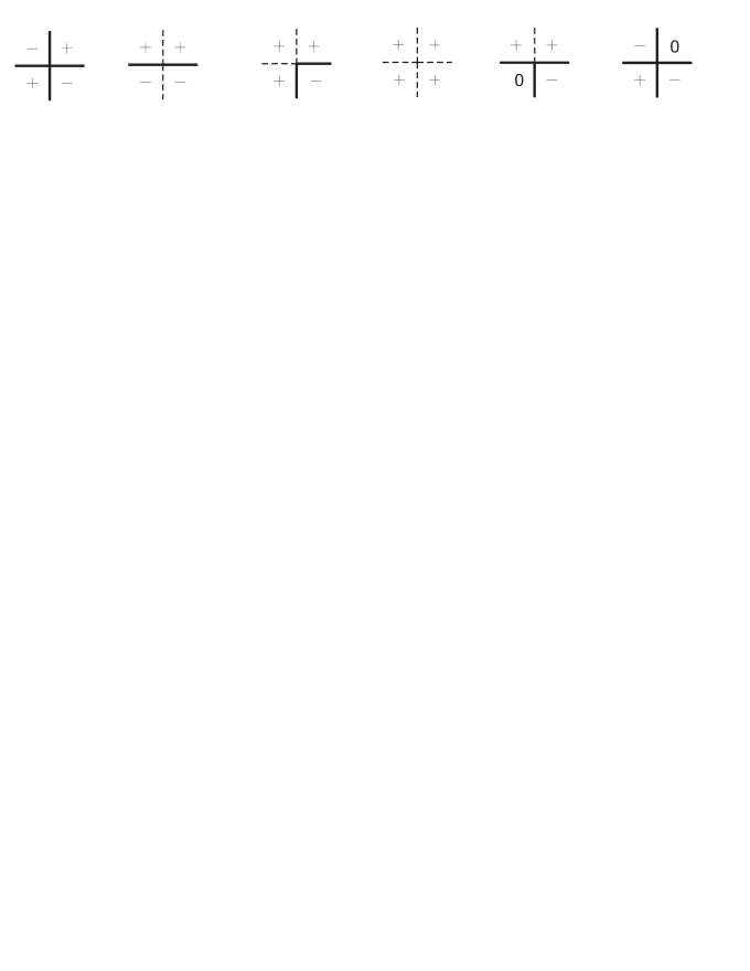
Figure 1: Different plaquette configurations on a given edge for the case $\sigma=0,\pm 1$ (here q=3). Plaquettes and the edges are drawn normal to the plane of the figure, the edge is at the center of the intersections. The spin variables are on the centers of the dual lattice. The corresponding energies are equal to $\varepsilon_{1}=4k,~{}\varepsilon_{2}=0,~{}\varepsilon_{3}=1,~{}\varepsilon_{4}=0,~{}\varepsilon_{5}=1,~{}\varepsilon_{6}=2k+1$ (from left to right). Only non-flat edges contribute to the energy functional $\varepsilon_{3}=\varepsilon_{5}=1$, the intersections are suppressed by a factor proportional to intersection coupling constant $k,$ $\varepsilon_{1}=4k,~{}\varepsilon_{6}=2k+1$.

3 Mean field analysis

It is useful to analyse our model using the mean field approximation, before employing the rather expensive Monte Carlo simulations. Since none of the $q$ states of the model is preferable over the others, one may assume that the fractions $x_{n}$ of the spins that take the value $n(n=0,\dots,q-1)$ may be expressed in the form:

$$x_{0}(s)=\frac{1+(q-1)s}{q},$$

$$~{}~{}x_{n}(s)=\frac{1-s}{q},n=1,\dots,q-1.$$ (5)

The order parameter $s$ will be the one which minimizes the free energy. The value $s=0$ induces equal values to the $x_{n}(s)$ while for $s=1$ we get $x_{0}(1)=1,x_{n}(1)=0,$ representing a long range order. With the remark that for each lattice site we have 3 first neighbours, 6 second neighbours and 3 plaquettes, we may easily write down the energy $E$ per site that enters in the mean field calculations:

$$E=(-2k)\cdot 3\cdot\sum_{n=0}^{q-1}x_{n}^{2}(s)+(\frac{k}{2})\cdot 6\cdot\sum_{n=0}^{q-1}x_{n}^{2}(s)+(-\frac{1-k}{2})\cdot 3\cdot\left(\frac{q\sum_{n=0}^{q-1}x_{n}^{2}(s)-1}{q-1}\right)^{2}$$ (6)

$$=-6k\sum_{n=0}^{q-1}x_{n}^{2}(s)+3k\sum_{n=0}^{q-1}x_{n}^{2}(s)-\frac{3(1-k)}{2}s^{4}$$ (7)

The sum representing the plaquette term has been written in the form indicated in equation (6), so that a $s^{4}$ term is reproduced. If one used the form $\left(\sum_{n=0}^{q-1}x_{n}^{2}(s)\right)^{2}$ instead, terms proportional to $s^{2}$ would also be present, contaminating the nearest neighbour terms. The calculations involves minimization of the free energy

$$F\equiv\beta E-S,$$

where the entropy $S$ is given by:

$$S=-\sum_{n=0}^{q-1}x_{n}(s)\ln(x_{n}(s)).$$

In Fig. 2 we show the mean field estimate of the critical temperature as a function of $k$ for $q=2,3,5.$ We observe that the critical temperature is highest (at the same value of $k$) for $q=2.$ In general the critical temperature increases with $k.$

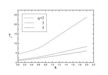
Figure 2: Mean Field result: Critical Temperature versus $k$ for various values of $q.$

A very interesting issue is the strength of the phase transition. This is quantified by the latent heat, which is essentially the entropy difference between the two phases accross the phase transition. The mean field predictions are contained in Fig.3. The striking feature is that for $q=2$ the latent heat starts from a (rather small) value and dives to zero as $k$ becomes bigger than about 0.8. Thus the prediction is that a first order transition becomes second order at some value of $k.$ This qualitatively agrees with known results about the standard gonihedric model. We note that this change takes actually place at $k\simeq 0.5,$ so the agreement is only approximate. This characteristic is not preserved for $q>2.$ It is evident from the figure that the latent heats for $q=3$ and $q=5$ are bigger than the ones for $q=2.$ The most important fact, however, is that the latent heats never become zero; instead they decrease monotonously with $k$ and eventually, for large enough $k$ there will be a weak first order transition which may not be easy to distinguish from a second order transition. We have checked that this is the case up to the value $k=10.$

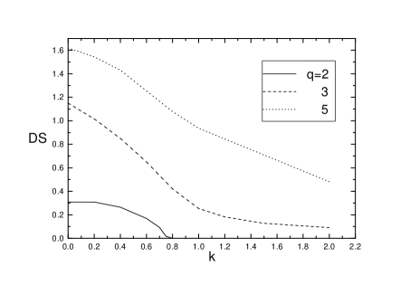
Figure 3: Mean Field result: Latent Heat versus $k$ for various values of $q.$

4 Monte Carlo Results

In this section we will study the gonihedric Potts model described by Eq. (4) using Monte Carlo techniques. The phase diagram of the model will obviously depend on $k$ and $q$. We consider the model for the values $k=0,\ 0.5$ and $1.0$ and $q>2$. In particular we will focus on $q=3,4,5.$ As we have explained, the $q=2$ case is equivalent to the standard gonihedric spin model, which has already been studied in the past. One of its main results for $q=2$ has been that the phase transition is of first order for small $k$ but it becomes of second order around $k=0.5.$ The mean field approach suggests that for $q>2$ the phase transition weakens, but it never becomes second order. We will check this issue with the Monte Carlo method. The outcome is that for $q>2$ the phase transition becomes of second order for quite bigger values of $k.$ In addition, we find out that the value of $k$ where the transition becomes second order depends on $q$ but in any case it is bigger than $1.0$ for $q>2.$ This is the last topic examined: we perform hysteresis loops for the values of $k:1.0,1.5,2.0,$ for $q=3$ and consider the changing magnitude of the loops.

We used a single flip Metropolis algorithm for the updating and imposed periodic boundary conditions.

4.1 The plaquette interaction case ($k=0$)

For $k=0$ only the last term in equation (4) contributes, so the Potts model has just the plaquette interaction. For the standard gonihedric model $(q=2)$ the system has a strong first order phase transition [4],[6]. The mean field results suggest that the order of the phase transition does not change for $q>2.$ To check the validity of this prediction we have studied the system using the hysteresis loop method. In Fig. 4 we present our results for energy versus temperature on a $20^{3}$ lattice volume for $q=3,4$. For comparison reasons we also plot the well known case for $q=2$. The unambiguous formation of large hysteresis loops accompanied by large jumps in energy in the critical region lead to a more or less safe conclusion of a first order phase transition. The critical temperature $T_{c}$ takes smaller values as $q$ increases and this feature is in qualitative agreement with the mean field prediction, which may be seen in Fig. 2.

Figure 4: Hysteresis loop results for $k=0$ and $q=2,3,4$ on a $20^{3}$ lattice volume.

4.2 The $k=0.5$ case

For this value of $k$ all three terms in the Hamiltonian contribute. We have chosen this value because, in the vicinity of $k=0.5,$ the phase transition of the $q=2$ case becomes second order [4]. In figure 4a we show the hysteresis loops for the energy versus the temperature for $q=2,3,4,5$ and a $20^{3}$ lattice. The absence of any loop for $q=2$ agrees with previous results indicating a second order phase transition. However, things change for $q>2:$ it is evident that the loops for $q=3,4,5$ grow bigger and the jump towards large values for the energy is clear at least for the $q=4,5$ cases. The conclusion suggested by the results in Fig. 4a is that at $k=0.5$ the phase transition is stronger for bigger $q.$ In Fig. 4b we show a two peak signal for $q=3$ for $10^{3}$ and $12^{3}$ lattice. The comparison for these two lattice volumes shows that for the $12^{3}$ lattice the separation between the two peaks is complete. This is a strong indication that we have a first order transition.

Figure 5: $k=0.5$: (a) Hysteresis loop results for $q=2,3,4,5$. (b) A two peak signal for $q=3$ on $10^{3}$ and $12^{3}$ lattice volumes.

4.3 Nearest and next-to-nearest neighbour interaction ($k=1.0$)

The plaquette interaction does not contribute in this case. A similar model for $q=3$, has been studied in the past [16, 17], and found to have a first order phase transition. The distinctive feature of the model we study here is that the ratio of the ferromagnetic and the antiferromagnetic couplings is four; this induces the huge degeneracy of the ground state that has been described above and is not shared by the model in references [16, 17]. It is of interest to detect if there are any consequences of this peculiar feature of the model.

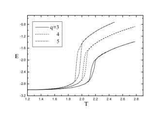
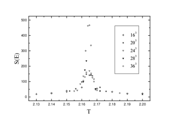
Figure 6: $k=1$: (a) Hysteresis loop results for $q=3,4,5$. (b) Susceptibility of the energy for five lattice volumes.(The statistical errors are small enough and they are not included for the figure not to be confused.)

The phase transition in the standard $q=2$ case is of second order [4], [7]. However, for bigger values of $q,$ the phase transition appears to be of first order. In Fig. 5a we depict the hysteresis loops for $q=3,4,5$ in a $20^{3}$ lattice. The clear loops for $q=4$ and $q=5$ give a strong indication for a first order phase transition. The $q=3$ case is not so clear, so in this case we also measure the susceptibility of the energy, $S(E)\equiv V(<E^{2}>-<E>^{2})$. The average energy has been measured over 200000-800000 measurements, sampling every fourth iteration. We have used five lattice volumes, namely $16^{3},20^{3},24^{3},28^{3}$ and $36^{3}$. The results depicted in Fig. 5b show that the peaks of the susceptibility increase almost linearly with the volume which is definitely the volume dependence characterizing a first order phase transition.

4.4 Larger values of $k$

On the basis of the results of the previous paragraph one would expect that the phase transition will possibly become of second order at some $k_{c}>1.$ Since the phase transition grows stronger with increasing $q,$ we expect that $k_{c}$ is an increasing function of $q.$ The precise evaluation of $k_{c}(q)$ would require heavy numerical work. Nevertheless, we can achieve qualitative understanding of the behaviour of the system. In Fig. 7 we depict the hysteresis loops for the $q=3$ Potts model at $k=1.0,\ 1.5,$ and $2.0$ on a $20^{3}$ lattice volume. As $k$ increases the loop gradually disappears. Thus the transition may become of second order at some value $k_{c}(3)$ greater than $1.0.$ Recalling that $k_{c}(2)\simeq 0.5,$ it appears that the hierarchy:

$$k_{c}(2)<k_{c}(3)<\dots.$$

might possibly be valid.

Figure 7: Hysteresis loop results on $20^{3}$ lattice volume for $q=3$ and $k=1.0,1.5,2.0.$

References

-
[1]
G.K. Savvidy and K.G. Savvidy. Phys.Lett. B337 (1994)
333;
Mod.Phys.Lett. A11 (1996) 1379
G.K. Savvidy, K.G. Savvidy and P.G. Savvidy. Phys.Lett. A221 (1996) 233
G. K. Savvidy, K. G. Savvidy and F. J. Wegner. Nucl.Phys. B443 (1995) 565. - [2] G.K. Bathas, E. Floratos, G.K. Savvidy and K.G. Savvidy, Modern Physics Letters A10 (1995) 2695 (hep-th/9504054).
- [3] D.Johnston and R.K.P.C. Malmini, Phys.Lett. B378 (1996) 87, Nucl.Phys.Proc.Suppl.53:773-776,1997.
-
[4]
M.Baig, D.Espriu,
D.Johnston and R.K.P.C.Malmini,
J.Phys. A30 (1997) 407 (hep-lat/9607002). - [5] A.Lipowski and D.Johnston, Glassy transition and metastability in four–spin Ising model (cond-mat/9812098).
- [6] A. Lipowski, J. Phys. A: Math. Gen. 30 (1997) 7365.
- [7] P.Dimopoulos, D. Espriu, E. Jane and A. Prats, Phys.Rev.E66:056112,2002 [cond-mat/0204403].
- [8] G.Koutsoumbas et.al. Phys.Lett. B410 (1997) 241.
-
[9]
A.Cappi, P.Colangelo, G.Gonnella and
A.Maritan, Nucl. Phys. B370 (1992) 659
G.Gonnella, S.Lise and A.Maritan, Europhys. Lett. 32 (1995) 735
E.N.M.Cirillo and G.Gonnella. J.Phys.A: Math.Gen.28 (1995) 867
E.N.M.Cirillo, G.Gonnella and A.Pelizzola, Phys.Rev. E55, R17 (1997)
E.N.M.Cirillo, G.Gonnella D.Johnston and A.Pelizzola, Phys.Lett. A226, 59 (1997)
E.N.M.Cirillo, G.Gonnella and A.Pelizzola, Nucl.Phys. (Proc.Suppl.) 63, 622 (1998)
-
[10]
T.Jonsson and G.K.Savvidy. Phys.Lett.B449
(1999) 254;
Nucl.Phys. B575 (2000) 661-672, hep-th/9907031 - [11] G.K.Savvidy. JHEP 0009 (2000) 044
-
[12]
G.K. Savvidy and K.G. Savvidy,
Int. J. Mod. Phys. A8 (1993) 3993
R.V. Ambartzumian, G.K. Savvidy , K.G. Savvidy and G.S. Sukiasian. Phys. Lett. B275 (1992) 99
G.K. Savvidy and K.G. Savvidy. Mod.Phys.Lett. A8 (1993) 2963
B.Durhuus and T.Jonsson. Phys.Lett. B297 (1992) 271 -
[13]
D.Weingarten. Nucl.Phys.B210 (1982) 229
A.Maritan and C.Omero. Phys.Lett. B109 (1982) 51
T.Sterling and J.Greensite. Phys.Lett. B121 (1983) 345
B.Durhuus,J.Fröhlich and T.Jonsson. Nucl.Phys.B225 (1983) 183
J.Ambjørn,B.Durhuus,J.Fröhlich and T.Jonsson. Nucl.Phys.B290 (1987) 480
T.Hofsäss and H.Kleinert. Phys.Lett. A102 (1984) 420
M.Karowski and H.J.Thun. Phys.Rev.Lett. 54 (1985) 2556
F.David. Europhys.Lett. 9 (1989) 575 - [14] F.J. Wegner, J. Math. Phys.12 (1971) 2259
-
[15]
G.K.Savvidy and F.J.Wegner. Nucl.Phys.B413(1994)605
G.K. Savvidy and K.G. Savvidy. Phys.Lett. B324 (1994) 72
R. Pietig and F.J. Wegner. Nucl.Phys. B466 (1996) 513 - [16] R.Gavai, F.Karsch, Phys.Lett.B233 (1989) 417.
- [17] A.Billoire, R.Lacaze, A.Morel, Nucl.Phys.B340 (1990) 542.