Nonlinear Realization of Chiral Symmetry
on the Lattice

Abstract

We formulate lattice theories in which chiral symmetry is realized nonlinearly on the fermion fields. In this framework the fermion mass term does not break chiral symmetry. This property allows us to use the Wilson term to remove the doubler fermions while maintaining exact chiral symmetry on the lattice. Our lattice formulation enables us to address non-perturbative questions in effective field theories of baryons interacting with pions and in models involving constituent quarks interacting with pions and gluons. We show that a system containing a non-zero density of static baryons interacting with pions can be studied on the lattice without encountering complex action problems. In our formulation one can also decide non-perturbatively if the chiral quark model of Georgi and Manohar provides an appropriate low-energy description of QCD. If so, one could understand why the non-relativistic quark model works.

Keywords: Chiral Quark Model, Chiral Symmetry, Lattice QCD, Low-Energy Effective Theories, Non-Zero Baryon Chemical Potential

PACS numbers: 11.30.Rd, 12.38.Gc, 12.38.Mh, 12.39.Fe

1 Introduction

Realizing chiral symmetry on the lattice is a problem with a long history. In 1975 Wilson decided to break chiral symmetry explicitly in order to remove the unwanted doubler fermions [1]. As a result, recovering chiral symmetry with Wilson fermions requires fine-tuning as well as taking the continuum limit. In 1981 it was proved by Nielsen and Ninomiya [2] and in a different way by Friedan [3] that removing the doubler fermions while maintaining locality is possible only if one explicitly breaks the chiral symmetry of the continuum theory. In 1992, using a Wilson term in 4+1 dimensions, Kaplan constructed domain wall fermions in order to realize chiral symmetry on the lattice [4]. At the end of the same year, Narayanan and Neuberger introduced the related overlap formulation of chiral lattice fermions [5]. Already in 1982 Ginsparg and Wilson [6] had discussed how to maintain a remnant of chiral symmetry on the lattice. This paper was rediscovered by Hasenfratz in 1997 in relation to the perfect action approach to QCD [7]. In particular, perfect lattice fermions obey the by now well-known Ginsparg-Wilson relation. It was immediately realized by Neuberger that the same is true for overlap fermions [8]. In 1998 Lüscher showed that lattice fermion actions that obey the Ginsparg-Wilson relation realize a new version of chiral symmetry that is natural for theories on the lattice and coincides with the usual one in the continuum limit [9]. This development culminated in the non-perturbative construction of chiral lattice gauge theories [10].

In this paper we consider another aspect of lattice chiral symmetry, namely how it can be realized nonlinearly. Nonlinear realizations of symmetries are well understood in the continuum in the context of low-energy effective theories describing spontaneous symmetry breaking. Goldstone’s theorem tells us that the spontaneous breakdown of a continuous global symmetry $G$ to an unbroken subgroup $H$ implies the presence of massless particles: the number of Goldstone boson fields is given by the difference between the number of generators of $G$ and $H$ [11]. The chiral symmetry group $G=SU(N_{f})_{L}\otimes SU(N_{f})_{R}\otimes U(1)_{B}$ of QCD with $N_{f}$ massless quark flavors is spontaneously broken to the vector subgroup $H=SU(N_{f})_{L=R}\otimes U(1)_{B}$. Hence there are $N_{f}^{2}-1$ massless Goldstone bosons: the three pions for $N_{f}=2$ and, in addition, the four kaons, and the $\eta$-meson for $N_{f}=3$. The theoretical framework for describing Goldstone bosons with effective fields was developed by Weinberg [12] and by Coleman, Wess, and Zumino [13], partly in collaboration with Callan [14]. As a result, Goldstone bosons are described by fields in the coset space $G/H$ and the group $G$ is nonlinearly realized on those fields. In QCD the pions, the kaons, and the $\eta$-meson are accordingly described by matrix valued fields in the coset space $G/H=SU(N_{f})_{L}\otimes SU(N_{f})_{R}\otimes U(1)_{B}/[SU(N_{f})_{L=R}\otimes U(1)_{B}]=SU(N_{f})$. Notably, the pion effective theory developed by Weinberg [15] has a systematic low-energy expansion in Gasser and Leutwyler’s framework of chiral perturbation theory [16].

When matter fields are included in the effective theory of Goldstone bosons, they also transform nonlinearly under chiral symmetry [17]. In particular, the global symmetry $G$ is hidden in a locally realized symmetry $H$ with a corresponding “gauge” field that is constructed from the Goldstone boson field. It must be pointed out that there is no true gauge symmetry $H$, just the global symmetry $G$. Exploiting a nonlinearly realized chiral symmetry, Gasser, Sainio, and Svarc incorporated a single nucleon in chiral perturbation theory [18]. Systematic power counting schemes for non-relativistic heavy baryon chiral perturbation theory were developed by Jenkins and Manohar [19] and by Bernard, Kaiser, Kambor, and Meissner [20]. A more economical scheme that maintains explicit Lorentz invariance was introduced by Becher and Leutwyler [21].

One may ask why one would want to put low-energy effective theories on the lattice. Indeed, many questions that arise in the framework of low-energy Lagrangians can be solved analytically using chiral perturbation theory. Usually, such calculations are performed in the continuum using dimensional regularization. It is certainly more tedious to work with the lattice regularization in chiral perturbation theory calculations. Still, in order to address conceptual problems, for example, related to power divergences, the lattice has already been used in magnon [22], pion [23], as well as heavy baryon chiral perturbation theory [24]. In the context of lattice QCD, effective field theories provide powerful tools to keep systematic errors under control [25]. Moreover, chiral Lagrangians on the lattice have been investigated in order to facilitate the lattice determination of the Gasser-Leutwyler coefficients [26, 27]. Although interesting, this is not the main motivation for the present work. We formulate lattice theories with nonlinearly realized chiral symmetry in order to address non-perturbative questions that arise in the context of low-energy effective theories. It is perhaps not obvious that such problems even exist. An example of a non-perturbative problem in the context of chiral Lagrangians concerns the rotor spectrum of massless QCD in a finite box. However, this problem reduces to one in quantum mechanics and has been solved analytically by Leutwyler [28] without any need for a lattice. Few-nucleon systems have been treated with effective field theory methods in nuclear physics. For example, the two-nucleon system was studied by Kaplan, Savage, and Wise [29] and the three-nucleon system was investigated by Bedaque, Hammer, and van Kolck [30, 31]. Again, the solution of these problems required non-perturbative techniques but not yet a lattice. Going to larger nuclei and eventually to nuclear matter is a non-trivial task that requires to solve more complicated non-perturbative problems in the effective theory [32]. Here the lattice provides a natural framework in which such questions can be addressed on a solid theoretical basis.

A central observation of this paper is that the Nielsen-Ninomiya theorem is naturally avoided when chiral symmetry is nonlinearly realized on the lattice. In fact, constituent quark masses do not break a nonlinearly realized chiral symmetry. Similarly, the Wilson term — introduced in order to remove the doubler fermions — does no longer break chiral symmetry explicitly. Hence, exact chiral symmetry is naturally maintained using a simple Wilson action while the fermion doubling problem is still solved. This raises the question how anomalies manifest themselves in this context. Remarkably, in effective theories with nonlinearly realized chiral symmetry, both in the continuum and on the lattice, the fermion fields do not contribute to anomalies. Instead anomalies must be added by hand in the form of Wess-Zumino-Witten [33, 34] and Goldstone-Wilczek [35] terms. Constructing these terms on the lattice while maintaining their topological features is a non-trivial problem which we do not address in this paper. In this respect, our construction of lattice theories with nonlinearly realized chiral symmetry is still incomplete. Consequently, we limit ourselves to applications where anomalies play no major role. Such applications concern, for example, models of static baryons interacting with pions at non-zero chemical potential and the chiral quark model of Georgi and Manohar [36].

Dynamical fermion simulations in a lattice theory with nonlinearly realized chiral symmetry may be substantially easier than with the usual linear realization. Using the nonlinear realization, even in the chiral limit, the fermion mass is large due to spontaneous chiral symmetry breaking. Hence, the simulated dynamical fermions should behave algorithmically like heavy Wilson fermions while still maintaining manifest chiral symmetry. Using a linear realization of chiral symmetry on the quark fields, explicit auxiliary pion fields have already been explored in order to simplify QCD simulations [37, 38]. It has to be mentioned that, in general, lattice theories with nonlinearly realized chiral symmetry have a potential sign problem similar to the one that arises for a single flavor of Wilson fermions. Fortunately, this sign problem is a lattice artifact which should disappear in the continuum limit, in particular, for sufficiently heavy fermions. Recently, without directly addressing the potential sign problem, dynamical fermion algorithms have been developed for an odd number of flavors of Wilson fermions [39, 40, 41, 42]. We expect that similar methods are applicable to lattice fermions with nonlinearly realized chiral symmetry. Still, it should be pointed out that the feasibility of dynamical fermion simulations depends crucially on the severity of the sign problem, which should be investigated in numerical simulations. We also need to mention that additional complex action problems arise if pseudo-vector fermion couplings or Wess-Zumino-Witten and Goldstone-Wilczek terms are included. In this paper we concentrate on the theoretical formulation of lattice theories with a nonlinearly realized chiral symmetry, while results of numerical simulations will be presented elsewhere.

Interestingly, the lattice construction presented here enables us to simulate massless pions interacting with static baryons even at non-zero baryon chemical potential $\mu$ and finite temperature $T$, both for two and for three flavors. In contrast to full QCD, in the static baryon model this is possible without encountering a complex action problem. Although questions involving high temperatures or high baryon densities are beyond the applicability of a systematic low-energy expansion, this model can still be used to answer questions concerning the universal features of the critical endpoint of the chiral phase transition line in the $(\mu,T)$-plane. Although one should not expect to obtain precise information on non-universal features of QCD, such as the location of the critical endpoint, one may learn at least semi-quantitatively how the location of the endpoint changes as a function of the strange quark mass. In addition, one will gain experience with numerical methods for locating the critical endpoint in a model that has the same global symmetry properties as full QCD but is much simpler to simulate.

A nonlinear realization of chiral symmetry was also used by Georgi and Manohar in the construction of their chiral quark model [36]. This model contains massive constituent quarks interacting with pions and gluons. While gluons are flavor singlets, both constituent quarks and pions transform non-trivially under the nonlinearly realized chiral symmetry. If this model provides an appropriate low-energy description for QCD, one could understand why the non-relativistic quark model works. However, the confinement of constituent quarks is a non-perturbative issue that cannot be addressed quantitatively in the continuum formulation of the model. In this paper we present a lattice construction of the Georgi-Manohar model with nonlinearly realized chiral symmetry. This non-perturbative framework will allow one to decide quantitatively if the Georgi-Manohar model can explain the success of the non-relativistic quark model.

The rest of this paper is organized as follows. In section 2 the nonlinear realization of chiral symmetry is reviewed in the continuum, while section 3 contains the corresponding construction on the lattice. In both cases the relevant symmetries are discussed in detail. In particular, effective lattice theories for pions and baryons are considered and the issue of fermion doubling is discussed. In section 4 we discuss how low-energy effective theories can be treated non-perturbatively on the lattice and how continuum results can be extracted. Section 5 explains how theories with static baryons can be simulated at non-zero chemical potential without encountering a complex action problem. In section 6 we discuss the lattice version of the Georgi-Manohar model and propose numerical simulations in order to decide if it indeed provides a satisfactory explanation for the success of the non-relativistic quark model. Section 7 discusses the possible form of the phase diagram of the lattice chiral quark model and the relation of this model to Wilson’s standard lattice QCD. Finally, section 8 contains our conclusions.

2 Continuum Formulation of Nonlinearly
Realized Chiral Symmetry

In this section we review how theories with nonlinearly realized chiral symmetry are formulated in the continuum. The fields used in this construction are introduced with emphasis on their behavior under chiral symmetry transformations, charge conjugation, and parity. Simple examples of low-energy effective theories with nonlinearly realized chiral symmetry are given and manifestations of anomalies are being discussed.

Consider the chiral symmetry group $G=SU(N_{f})_{L}\otimes SU(N_{f})_{R}\otimes U(1)_{B}$ of QCD involving $N_{f}$ quark flavors which breaks spontaneously to the subgroup $H=SU(N_{f})_{L=R}\otimes U(1)_{B}$. Following [13, 14] the Goldstone boson field is then given by $U(x)=\exp[2i\pi^{a}(x)T^{a}/F_{\pi}]\in G/H=SU(N_{f})$. Here $\mbox{Tr}(T^{a}T^{b})=2\delta_{ab}$ and $F_{\pi}$ is the pion decay constant. Under global chiral rotations $L\otimes R\in SU(N_{f})_{L}\otimes SU(N_{f})_{R}$, this field transforms as

$$U(x)^{\prime}=LU(x)R^{\dagger}.$$ (2.1)

From the Goldstone boson field one derives a field $u(x)\in SU(N_{f})$ as

$$u(x)=U(x)^{1/2}.$$ (2.2)

In order to avoid ambiguities in taking the square-root, we proceed as follows. First, the field $U(x)$ is diagonalized by a unitary transformation $W(x)$, i.e.

$$U(x)=W(x)D(x)W(x)^{\dagger},$$ (2.3)

where $D(x)$ is a diagonal matrix of complex phases

$$D(x)=\mbox{diag}\{\exp[i\varphi_{1}(x)],\exp[i\varphi_{2}(x)],...,\exp[i\varphi_{N_{f}}(x)]\}.$$ (2.4)

At this point, the phases $\varphi_{i}(x)$ are defined only modulo $2\pi$. In order to fix this ambiguity, we demand that

$$\sum_{i=1}^{N_{f}}\varphi_{i}(x)=0,\ |\varphi_{i}(x)-\varphi_{j}(x)|\leq 2\pi.$$ (2.5)

This uniquely fixes the phases of the eigenvalues and defines the matrix $D(x)$ up to an irrelevant permutation of its diagonal elements. We then define

$$D(x)^{1/2}=\mbox{diag}\{\exp[i\varphi_{1}(x)/2],\exp[i\varphi_{2}(x)/2],...,\exp[i\varphi_{N_{f}}(x)/2]\},$$ (2.6)

and we obtain

$$u(x)=W(x)D(x)^{1/2}W(x)^{\dagger}.$$ (2.7)

When the eigenvalues of $U(x)$ are non-degenerate, the matrix $u(x)$ is uniquely defined in this way and is located in the middle of the shortest geodesic connecting $U(x)$ with the unit-matrix ${\sf 1\!\!1}$ in the group manifold of $SU(N_{f})$. On the other hand, if two eigenvalues are degenerate, the corresponding eigenvectors are not uniquely defined. If, in addition, the corresponding phases $\varphi_{i}$ and $\varphi_{j}$ differ by $2\pi$, this ambiguity gives rise to a coordinate singularity in the definition of $u(x)$. In the $N_{f}=2$ case, the singularities arise for $U(x)=-{\sf 1\!\!1}$, which corresponds to a single point in the $SU(2)$ group manifold. For general $N_{f}$, the submanifold of $SU(N_{f})$ matrices with two degenerate eigenvalues (and with $|\varphi_{i}-\varphi_{j}|=2\pi$) has dimension $N_{f}^{2}-4$. Hence, the codimension of the singular submanifold is $N_{f}^{2}-1-(N_{f}^{2}-4)=3$ for all $N_{f}$. Consequently, in a 4-dimensional space-time the singularities in $u(x)$ are located on 1-dimensional lines. If one chooses the vacuum as $U(x)={\sf 1\!\!1}$, the singularities represent the world-lines of Skyrmion centers. However, it should be noted that the location of the singularities varies under those chiral rotations that do not leave the vacuum invariant. Still, the effective actions that we will construct with $u(x)$ are completely chirally invariant, even in the presence of Skyrmions or other large-field configurations.

Under chiral rotations the field $u(x)$ transforms as

$$u(x)^{\prime}=Lu(x)V(x)^{\dagger}=V(x)u(x)R^{\dagger}.$$ (2.8)

The matrix $V(x)$ depends on $L$ and $R$ as well as on the field $U(x)$ and can be written as

$$V(x)=R[R^{\dagger}LU(x)]^{1/2}[U(x)^{1/2}]^{\dagger}=L[L^{\dagger}RU(x)^{\dagger}]^{1/2}U(x)^{1/2}.$$ (2.9)

For transformations in the unbroken vector subgroup $SU(N_{f})_{L=R}$, $L=R$, the field $V(x)$ reduces to the global flavor transformation $V(x)=L=R$. The local transformation $V(x)$ is a nonlinear representation of chiral symmetry. For two subsequent chiral transformations with $L_{2}L_{1}=L$ and $R_{2}R_{1}=R$, one has

$$V_{1}(x)=R_{1}[R_{1}^{\dagger}L_{1}U(x)]^{1/2}[U(x)^{1/2}]^{\dagger},\ V_{2}(x)=R_{2}[R_{2}^{\dagger}L_{2}U(x)^{\prime}]^{1/2}[{U(x)^{\prime}}^{1/2}]^{\dagger},$$ (2.10)

with $U(x)^{\prime}=L_{1}U(x)R_{1}^{\dagger}$, so that indeed

$$V_{2}(x)V_{1}(x) = R_{2}[R_{2}^{\dagger}L_{2}L_{1}U(x)R_{1}^{\dagger}]^{1/2}R_{1}[U(x)^{1/2}]^{\dagger}$$ (2.11)

$$= R_{2}R_{1}[R_{1}^{\dagger}R_{2}^{\dagger}L_{2}L_{1}U(x)]^{1/2}[U(x)^{1/2}]^{\dagger}$$

$$= R[R^{\dagger}LU(x)]^{1/2}[U(x)^{1/2}]^{\dagger}=V(x).$$

Now consider a Dirac spinor field $\Psi(x)$ and $\overline{\Psi}(x)$ that transforms under the fundamental representation of the flavor group. This field may represent a nucleon (for $N_{f}=2$) or a constituent quark (for any value of $N_{f}$). Global chiral rotations $L\otimes R\in SU(N_{f})_{L}\otimes SU(N_{f})_{R}$ can be realized nonlinearly on this field using the transformations

$$\Psi(x)^{\prime}=V(x)\Psi(x),\ \overline{\Psi}(x)^{\prime}=\overline{\Psi}(x)V(x)^{\dagger}.$$ (2.12)

This has the form of an $SU(N_{f})$ gauge transformation despite the fact that it represents just a global $SU(N_{f})_{L}\otimes SU(N_{f})_{R}$ symmetry.

In order to construct a chirally invariant (i.e. $SU(N_{f})$ “gauge” invariant) Lagrangian, one needs an $SU(N_{f})$ flavor “gauge” field. Indeed, the anti-Hermitean composite field

$$v_{\mu}(x)=\frac{1}{2}[u(x)^{\dagger}\partial_{\mu}u(x)+u(x)\partial_{\mu}u(x)^{\dagger}]$$ (2.13)

transforms as a “gauge” field

$$v_{\mu}(x)^{\prime} = \frac{1}{2}\{V(x)u(x)^{\dagger}L^{\dagger}\partial_{\mu}[Lu(x)V(x)^{\dagger}]+V(x)u(x)R^{\dagger}\partial_{\mu}[Ru(x)^{\dagger}V(x)^{\dagger}]\}$$ (2.14)

$$= V(x)[v_{\mu}(x)+\partial_{\mu}]V(x)^{\dagger}.$$

A Hermitean composite field is given by

$$a_{\mu}(x)=\frac{i}{2}[u(x)^{\dagger}\partial_{\mu}u(x)-u(x)\partial_{\mu}u(x)^{\dagger}],$$ (2.15)

which transforms as

$$a_{\mu}(x)^{\prime} = \frac{1}{2}\{V(x)u(x)^{\dagger}L^{\dagger}\partial_{\mu}[Lu(x)V(x)^{\dagger}]-V(x)u(x)R^{\dagger}\partial_{\mu}[Ru(x)^{\dagger}V(x)^{\dagger}]\}$$ (2.16)

$$= V(x)a_{\mu}(x)V(x)^{\dagger}.$$

It is interesting to investigate the transformation properties of the fields $\Psi(x)$, $\overline{\Psi}(x)$, $U(x)$, $u(x)$, $v_{\mu}(x)$, and $a_{\mu}(x)$ under charge conjugation and parity. Under charge conjugation, the fermion field transforms in the usual way

$$^{C}\Psi(x)=C\overline{\Psi}(x)^{T},\ ^{C}\overline{\Psi}(x)=-\Psi(x)^{T}C^{-1},$$ (2.17)

with $C^{-1}\gamma_{\mu}C=-\gamma_{\mu}^{T}$. The Goldstone boson field $U(x)$ transforms as

$${}^{C}U(x)=U(x)^{T}.$$ (2.18)

Consequently, the field $u(x)$ also follows the same transformation law

$${}^{C}u(x)=[^{C}U(x)]^{1/2}=[U(x)^{T}]^{1/2}=[U(x)^{1/2}]^{T}=u(x)^{T}.$$ (2.19)

It is easy to show that the composite fields $v_{\mu}(x)$ and $a_{\mu}(x)$ transform as

$${}^{C}v_{\mu}(x)=v_{\mu}(x)^{*},\ ^{C}a_{\mu}(x)=a_{\mu}(x)^{*}.$$ (2.20)

Under parity, the fermion field behaves again in the usual way, i.e.

$${}^{P}\Psi(\vec{x},t)=\gamma_{4}\Psi(-\vec{x},t),\ ^{P}\overline{\Psi}(\vec{x},t)=\overline{\Psi}(-\vec{x},t)\gamma_{4},$$ (2.21)

where 4 denotes the Euclidean time direction. The Goldstone boson field $U(x)$ transforms as

$${}^{P}U(\vec{x},t)=U(-\vec{x},t)^{\dagger}$$ (2.22)

so that

$${}^{P}u(\vec{x},t)=[^{P}U(\vec{x},t)]^{1/2}=[U(-\vec{x},t)^{\dagger}]^{1/2}=[U(-\vec{x},t)^{1/2}]^{\dagger}=u(-\vec{x},t)^{\dagger}.$$ (2.23)

Similarly, one finds

$${}^{P}v_{i}(\vec{x},t)=-v_{i}(-\vec{x},t),\ ^{P}v_{4}(\vec{x},t)=v_{4}(-\vec{x},t),$$

$${}^{P}a_{i}(\vec{x},t)=a_{i}(-\vec{x},t),\ ^{P}a_{4}(\vec{x},t)=-a_{4}(-\vec{x},t),$$ (2.24)

where $i\in\{1,2,3\}$ denotes a spatial direction. Hence, $v_{\mu}(x)$ is a vector and $a_{\mu}(x)$ is an axial vector.

At this point we are prepared to write down the leading terms in the Euclidean action of a low-energy effective theory for nucleons (with $N_{f}=2$)

$$S[\overline{\Psi},\Psi,U] = \int d^{4}x\ \Big{\{}M\overline{\Psi}\Psi+\overline{\Psi}\gamma_{\mu}(\partial_{\mu}+v_{\mu})\Psi+ig_{A}\overline{\Psi}\gamma_{\mu}\gamma_{5}a_{\mu}\Psi$$ (2.25)

$$+ \frac{F_{\pi}^{2}}{4}\mbox{Tr}[\partial_{\mu}U^{\dagger}\partial_{\mu}U]-\frac{\langle\overline{\psi}\psi\rangle}{2}\mbox{Tr}[{\cal M}U^{\dagger}+{\cal M}^{\dagger}U]\Big{\}}.$$

Here $M$ is the nucleon mass generated by spontaneous chiral symmetry breaking, $g_{A}$ is the coupling to the isovector axial current, and $\langle\overline{\psi}\psi\rangle$ and ${\cal M}=\mbox{diag}(m_{u},m_{d})$ are respectively the chiral condensate per flavor and the mass matrix of the current quarks. When $\Psi(x)$ represents a constituent quark, $M$ would be the constituent quark mass. In that case, gluons must also be included in order to confine the constituent quarks. This is what happens in the chiral quark model of Georgi and Manohar [36] (see section 6).

It is remarkable that — due to the nonlinear realization of chiral symmetry — the fermion mass term is chirally invariant. This makes sense because the mass $M$ arises from the spontaneous breakdown of chiral symmetry even in the chiral limit, i.e. when the current quarks are massless. In fact, the term that contains the matrix ${\cal M}$ of current quark masses is the only source of explicit chiral symmetry breaking in the leading terms of the effective theory. It is interesting to note that the composite field $v_{\mu}(x)$ is coupled to the fermions as a flavor “gauge” field that enters the covariant derivative $D_{\mu}=\partial_{\mu}+v_{\mu}$. Like $v_{\mu}$, the axial vector field $a_{\mu}$ also transforms in the adjoint representation of the flavor group. However, it is not a “gauge” field and it couples to the fermions with strength $g_{A}$. It must be noted that there is, of course, no true $SU(N_{f})$ gauge symmetry, just an $SU(N_{f})_{L}\otimes SU(N_{f})_{R}\otimes U(1)_{B}$ global symmetry. In particular, the “gauge” field $v_{\mu}(x)$ is not a fundamental field and there is, for instance, no $SU(N_{f})$ Gauss law.

Until now we have considered a fermion field $\Psi(x)$ transforming in the fundamental representation of $SU(N_{f})$. In QCD with three massless flavors ($N_{f}=3$) the baryons transform as a flavor octet. The corresponding Dirac spinor field, denoted by $\chi(x)$ and $\overline{\chi}(x)$, is traceless and transforms in the adjoint representation

$$\chi(x)^{\prime}=V(x)\chi(x)V(x)^{\dagger}.$$ (2.26)

The covariant derivative is then given by

$$D_{\mu}\chi(x)=\partial_{\mu}\chi(x)+[v_{\mu}(x),\chi(x)],$$ (2.27)

which transforms as $D_{\mu}\chi(x)^{\prime}=V(x)D_{\mu}\chi(x)V(x)^{\dagger}$ under the nonlinearly realized chiral symmetry. In this case, the Euclidean action of the effective theory for pions, kaons, $\eta$-mesons, and baryons takes the form

$$S[\overline{\chi},\chi,U] = \int d^{4}x\ \Big{\{}\mbox{Tr}[M\overline{\chi}\chi+\overline{\chi}\gamma_{\mu}D_{\mu}\chi+iD\overline{\chi}\gamma_{\mu}\gamma_{5}\{a_{\mu},\chi\}+iF\overline{\chi}\gamma_{\mu}\gamma_{5}[a_{\mu},\chi]]$$ (2.28)

$$+ \frac{F_{\pi}^{2}}{4}\mbox{Tr}[\partial_{\mu}U^{\dagger}\partial_{\mu}U]-\frac{\langle\overline{\psi}\psi\rangle}{2}\mbox{Tr}[{\cal M}U^{\dagger}+{\cal M}^{\dagger}U]\Big{\}},$$

where the matrix ${\cal M}=\mbox{diag}(m_{u},m_{d},m_{s})$ now also includes the strange quark mass. The low-energy parameters $D$ and $F$ are analogous to the coupling $g_{A}$ of the two flavor case.

It is interesting to discuss how anomalies arise in effective theories with nonlinearly realized chiral symmetry. Let us begin with a discussion of the axial $U(1)_{A}$ symmetry of QCD. When the number of colors $N_{c}$ is finite, this symmetry of the classical action is anomalously broken by quantum effects due to instantons [43]. As a result, the $\eta^{\prime}$-meson is not a Goldstone boson. Only in the large $N_{c}$ limit the $\eta^{\prime}$-meson becomes a pseudo-Goldstone boson [45, 44]. For $N_{c}=3$, the $U(1)_{A}$ symmetry is so strongly broken that it cannot even be considered an approximate symmetry of QCD. In particular, the $\eta^{\prime}$-meson is so heavy that it is not included explicitly in the low-energy effective theory. Indeed, the effective theories that we have written down do not have a $U(1)_{A}$ symmetry at all. This follows because the Goldstone boson field lives in $SU(N_{f})$ and not in $U(N_{f})$.

Let us now move on to those anomalies that arise when one gauges the electroweak interactions. In effective theories with nonlinearly realized chiral symmetries anomalies manifest themselves [17] in the form of Wess-Zumino-Witten [33, 34] and Goldstone-Wilczek terms [35]. For example, in the $N_{f}=2$ case, Witten’s global $SU(2)_{L}$ anomaly [46] manifests itself in a topological factor $\mbox{Sign}[U]^{N_{c}}\in\Pi_{4}[SU(2)]=\{1,-1\}$ that must be included in the path integral [47]. This ensures that, for odd $N_{c}$, the Skyrme soliton [48] is quantized as a fermion representing the physical nucleon in the pure pion theory. The $SU(2)_{L}$ gauge invariant version of the Skyrme baryon number current is the Goldstone-Wilczek current [35]. In the presence of electroweak instantons, this current is no longer conserved and reproduces the ’t Hooft anomaly in the baryon number [43].

In the $N_{f}\geq 3$ case, the Wess-Zumino-Witten term replaces the topological factor $\mbox{Sign}[U]$ in the Goldstone boson theory. This is because then $\Pi_{4}[SU(N_{f})]=\{0\}$ and instead $\Pi_{5}[SU(N_{f})]={\sf Z\!\!\!Z}$. The Wess-Zumino-Witten action has the form

$$S_{WZW}[U]=\frac{1}{240\pi^{2}i}\int_{H^{5}}d^{5}x\ \varepsilon_{\mu\nu\rho\sigma\lambda}\mbox{Tr}[(U^{\dagger}\partial_{\mu}U)(U^{\dagger}\partial_{\nu}U)(U^{\dagger}\partial_{\rho}U)(U^{\dagger}\partial_{\sigma}U)(U^{\dagger}\partial_{\lambda}U)],$$ (2.29)

where $H^{5}$ is a 5-dimensional hemi-sphere whose boundary $\partial H^{5}=S^{4}$ is (compactified) space-time. The physical Goldstone boson field $U(x)\in SU(N_{f})$ is extended to a field $U(x,x_{5})$ that depends on the unphysical fifth coordinate $x_{5}\in[0,1]$ such that $U(x,0)={\sf 1\!\!1}$ and $U(x,1)=U(x)$. Of course, the 4-dimensional physics should be independent of how the field $U(x,x_{5})$ is deformed into the bulk of the fifth dimension, and should only depend on $U(x)$. This is possible because the interpolation ambiguity of $S_{WZW}[U]$ is given by $2\pi$ times a winding number in $\Pi_{5}[SU(N_{f})]={\sf Z\!\!\!Z}$. Hence, when the prefactor of the Wess-Zumino-Witten term is quantized in integer units, the 4-dimensional physics is independent of how one interpolates the Goldstone boson field into the unphysical fifth dimension. Remarkably, in the low-energy theory for QCD, the quantized prefactor is the number of colors $N_{c}$ so that

$$Z=\int{\cal D}U\exp(-S[U])\exp(iN_{c}S_{WZW}[U]).$$ (2.30)

For $N_{f}=2$, one can show that $\exp(iN_{c}S_{WZW}[U])=\mbox{Sign}[U]^{N_{c}}$. The Wess-Zumino-Witten term contains the vertex that describes the anomalous decay of the neutral pion into two photons. For general $N_{c}$, this process also receives contributions from a Goldstone-Wilczek term [49].

In contrast to the $N_{f}=2$ case, for $N_{f}\geq 3$, the Wess-Zumino-Witten term also breaks an unwanted intrinsic parity symmetry $P_{0}$ that is present in the Goldstone boson action $S[U]$ but not in QCD [34]. The full parity $P$ acts on the pseudo-scalar Goldstone bosons $\pi^{a}(\vec{x},t)$ by spatial inversion accompanied by a sign-change, i.e. ${}^{P}\pi^{a}(\vec{x},t)=-\pi^{a}(-\vec{x},t)$, such that

$${}^{P}U(\vec{x},t)=U(-\vec{x},t)^{\dagger}.$$ (2.31)

The intrinsic parity $P_{0}$, on the other hand, leaves out the spatial inversion and takes the form

$${}^{P_{0}}U(\vec{x},t)=U(\vec{x},t)^{\dagger}.$$ (2.32)

If $P_{0}$ were a symmetry of QCD, the number of Goldstone bosons would be conserved modulo two. While this is indeed the case for $N_{f}=2$ (where $P_{0}$ is nothing but $G$-parity [50]), for $N_{f}\geq 3$ intrinsic parity is not a symmetry of QCD. For example, the $\phi$-meson can decay both into two kaons or into three pions. However, the Goldstone boson action $S[U]$ is indeed invariant under $P_{0}$,

$$S[^{P_{0}}U]=S[U^{\dagger}]=S[U].$$ (2.33)

Hence it has more symmetry than the underlying QCD action. The Wess-Zumino-Witten action, on the other hand, is odd under $P_{0}$,

$$S_{WZW}[^{P_{0}}U]=S_{WZW}[U^{\dagger}]=-S_{WZW}[U],$$ (2.34)

and thus reduces the symmetry of the effective theory to the one of QCD.

The next step is to ask how anomalies are represented when explicit baryon fields are present in the low-energy effective theory. In the presence of electroweak $SU(2)_{L}\otimes U(1)_{Y}$ gauge fields $W_{\mu}(x)=igW_{\mu}^{a}(x)T^{a}$ and $B_{\mu}(x)=ig^{\prime}B_{\mu}^{3}(x)T^{3}$ one obtains

$$v_{\mu}(x)=\frac{1}{2}\{u(x)^{\dagger}[\partial_{\mu}+W_{\mu}(x)]u(x)+u(x)[\partial_{\mu}+B_{\mu}(x)]u(x)^{\dagger}\},$$

$$a_{\mu}(x)=\frac{i}{2}\{u(x)^{\dagger}[\partial_{\mu}+W_{\mu}(x)]u(x)-u(x)[\partial_{\mu}+B_{\mu}(x)]u(x)^{\dagger}\},$$ (2.35)

which still transform as

$$v_{\mu}(x)^{\prime}=V(x)[v_{\mu}(x)+\partial_{\mu}]V(x)^{\dagger},\ a_{\mu}(x)^{\prime}=V(x)a_{\mu}(x)V(x)^{\dagger}.$$ (2.36)

Hence, the dynamical gauge fields $W_{\mu}(x)$ and $B_{\mu}(x)$ are incorporated in the “gauge” field $v_{\mu}(x)$ constructed from the pion field $U(x)$. By varying the resulting action with respect to $W_{\mu}(x)$ and $B_{\mu}(x)$, one obtains the left- and right-handed fermion currents

$$j_{\mu L}^{a}(x)=\overline{\Psi}(x)u(x)^{\dagger}\gamma_{\mu}\frac{1-g_{A}\gamma_{5}}{2}T^{a}u(x)\Psi(x),$$

$$j_{\mu R}^{a}(x)=\overline{\Psi}(x)u(x)\gamma_{\mu}\frac{1+g_{A}\gamma_{5}}{2}T^{a}u(x)^{\dagger}\Psi(x).$$ (2.37)

Since fermions with a nonlinearly realized chiral symmetry do not contribute to anomalies [17, 51], even in the presence of fermion fields, the anomalies are still contained in Goldstone-Wilczek and Wess-Zumino-Witten terms.

With explicit baryon fields being present in addition to the Skyrme solitons in the pion field, one may wonder if baryons are doubly counted in this approach. First of all, in the power counting scheme of chiral perturbation theory one cannot address questions about Skyrmions because all contributions from higher order terms are then equally important. In a non-perturbative approach to the effective theory, one can ask if, for example, in the sector with one baryon, the perturbative vacuum configuration of the pion field becomes unstable against Skyrmion formation. If so, the chiral power counting scheme is not applicable and the systematic low-energy approach fails. Hence, in the low-energy effective theory, one is restricted to the trivial topological sector and the issue of double counting does not arise. Since Skyrmions have no place in the systematic low-energy expansion, one cannot use the Goldstone-Wilczek current to describe baryon number violating processes in the framework of chiral perturbation theory. This should not be too surprising. Baryon decay — as rare as it may be — is a violent event that releases a lot of energy and can hence not be understood within a low-energy effective theory.

3 Lattice Formulation of Nonlinearly Realized
Chiral Symmetry

Let us now construct theories with a nonlinearly realized chiral symmetry on the lattice. In analogy to the previous section, we set up the lattice fields needed for this construction such that the correct symmetry properties are respected. With these fields, we formulate lattice actions of low-energy effective theories in which chiral symmetry is nonlinearly realized. In particular, we discuss how fermion doublers can be removed using a Wilson term without explicitly breaking chiral symmetry and how the Nielsen-Ninomiya theorem is avoided. The issue of anomalies is also addressed in the lattice formulation.

The Goldstone boson field $U_{x}\in SU(N_{f})$ lives on the sites $x$ of a 4-dimensional hyper-cubic lattice and it transforms under global chiral rotations as

$$U_{x}^{\prime}=LU_{x}R^{\dagger}.$$ (3.1)

As in the continuum, the field $u_{x}\in SU(N_{f})$ is constructed as $u_{x}=U_{x}^{1/2}$ and it transforms as

$$u_{x}^{\prime}=Lu_{x}V_{x}^{\dagger}=V_{x}u_{x}R^{\dagger}.$$ (3.2)

Again, the field $V_{x}$ depends on the global chiral transformations $L$ and $R$ as well as on the field $U_{x}$ and is given by

$$V_{x}=R(R^{\dagger}LU_{x})^{1/2}(U_{x}^{1/2})^{\dagger}=L(L^{\dagger}RU_{x}^{\dagger})^{1/2}U_{x}^{1/2}.$$ (3.3)

The continuum results for two subsequent chiral transformations given in eqs. (2.10) and (2.11) remain completely unchanged on the lattice. Also the discussion of the coordinate singularities still applies. However, it should be noted that the singularities generically fall between lattice points. Still, using an appropriate interpolation, it is possible to detect these topological objects even on the lattice.

Next we consider the fermion field $\Psi_{x}$ and $\overline{\Psi}_{x}$ which again lives on the lattice sites $x$. As in the continuum, global chiral rotations are nonlinearly realized on this field such that

$$\Psi_{x}^{\prime}=V_{x}\Psi_{x},\ \overline{\Psi}_{x}^{\prime}=\overline{\Psi}_{x}V_{x}^{\dagger}.$$ (3.4)

This field transforms in the fundamental representation of $SU(N_{f})$ and can hence represent a nucleon (for $N_{f}=2$) or a constituent quark (for any value of $N_{f}$). For $N_{f}=3$, the lattice baryon field $\chi_{x}$ and $\overline{\chi}_{x}$ also lives on the lattice sites but transforms in the adjoint representation

$$\chi_{x}^{\prime}=V_{x}\chi_{x}V_{x}^{\dagger},\ \overline{\chi}_{x}^{\prime}=V_{x}\overline{\chi}_{x}V_{x}^{\dagger}.$$ (3.5)

We now proceed to the construction of $V_{x,\mu}\in SU(N_{f})$ — the lattice analog of the continuum flavor “gauge” field $v_{\mu}(x)$. It should be noted that $V_{x,\mu}$ is a flavor parallel transporter along a lattice link in the group $SU(N_{f})$, while the continuum flavor “gauge” field is in the algebra $su(N_{f})$. In analogy to the continuum expression (2.13) for $v_{\mu}(x)$, we construct the lattice object

$$\tilde{V}_{x,\mu}=\frac{1}{2}[u_{x}^{\dagger}u_{x+\hat{\mu}}+u_{x}u_{x+\hat{\mu}}^{\dagger}].$$ (3.6)

Here $\hat{\mu}$ is the unit-vector in the $\mu$-direction. By construction, $\tilde{V}_{x,\mu}$ transforms as a parallel transporter under the nonlinearly realized chiral symmetry, i.e.

$$\tilde{V}_{x,\mu}^{\prime}=V_{x}\tilde{V}_{x,\mu}V_{x+\hat{\mu}}^{\dagger}.$$ (3.7)

In the classical continuum limit, $\tilde{V}_{x,\mu}=\exp[v_{\mu}(x+\hat{\mu}/2)]$. However, at finite lattice spacing, $\tilde{V}_{x,\mu}$ is in general not an element of $SU(N_{f})$, just a complex $N_{f}\times N_{f}$ matrix in the group $GL(N_{f})$. Hence, it is natural to project a group-valued parallel transporter $V_{x,\mu}\in SU(N_{f})$ out of $\tilde{V}_{x,\mu}$ by performing a $GL(N_{f})/SU(N_{f})$ coset decomposition

$$\tilde{V}_{x,\mu}=H_{x,\mu}\exp(i\varphi_{x,\mu}/N_{f})V_{x,\mu}.$$ (3.8)

Here

$$H_{x,\mu}=(\tilde{V}_{x,\mu}\tilde{V}_{x,\mu}^{\dagger})^{1/2}$$ (3.9)

is a positive Hermitean matrix that transforms as

$$H_{x,\mu}^{\prime}=V_{x}H_{x,\mu}V_{x}^{\dagger},$$ (3.10)

and $\exp(i\varphi_{x,\mu})$ (with $\varphi_{x,\mu}\in\ ]\!-\pi,\pi]$) is the phase of the determinant of $\tilde{V}_{x,\mu}$. Then, by construction,

$$V_{x,\mu}=\exp(-i\varphi_{x,\mu}/N_{f})H_{x,\mu}^{-1}\tilde{V}_{x,\mu},$$ (3.11)

is indeed in $SU(N_{f})$ and transforms as

$$V_{x,\mu}^{\prime}=V_{x}V_{x,\mu}V_{x+\hat{\mu}}^{\dagger}.$$ (3.12)

We also want to construct a lattice version of the continuum field $a_{\mu}(x)$ defined in (2.15). For this purpose, we first consider

$$\tilde{A}_{x,\mu}=\frac{i}{2}[u_{x}^{\dagger}u_{x+\hat{\mu}}-u_{x}u_{x+\hat{\mu}}^{\dagger}].$$ (3.13)

While in the continuum $a_{\mu}(x)^{\prime}=V(x)a_{\mu}(x)V(x)^{\dagger}$, the lattice field $\tilde{A}_{x,\mu}$ transforms as

$$\tilde{A}_{x,\mu}^{\prime}=V_{x}\tilde{A}_{x,\mu}V_{x+\hat{\mu}}^{\dagger}.$$ (3.14)

Also, in contrast to the continuum field $a_{\mu}(x)$, the lattice field $\tilde{A}_{x,\mu}$ is in general neither traceless nor Hermitean. To cure these problems, it is natural to introduce the field

$$A^{L}_{x,\mu}=\frac{1}{2}[\tilde{A}_{x,\mu}V_{x,\mu}^{\dagger}+V_{x,\mu}\tilde{A}_{x,\mu}^{\dagger}]-\frac{1}{2N_{f}}\mbox{Tr}[\tilde{A}_{x,\mu}V_{x,\mu}^{\dagger}+V_{x,\mu}\tilde{A}_{x,\mu}^{\dagger}]{\sf 1\!\!1},$$ (3.15)

which, by construction, is indeed traceless and Hermitean and which transforms as

$${A^{L}_{x,\mu}}^{\prime}=V_{x}A^{L}_{x,\mu}V_{x}^{\dagger},$$ (3.16)

with the matrix $V_{x}$ located at the site $x$ on the left end of the link $(x,\mu)$. Similarly, we define the object

$$A^{R}_{x,\mu}=\frac{1}{2}[V_{x,\mu}^{\dagger}\tilde{A}_{x,\mu}+\tilde{A}_{x,\mu}^{\dagger}V_{x,\mu}]-\frac{1}{2N_{f}}\mbox{Tr}[V_{x,\mu}^{\dagger}\tilde{A}_{x,\mu}+\tilde{A}_{x,\mu}^{\dagger}V_{x,\mu}]{\sf 1\!\!1},$$ (3.17)

which transforms as

$${A^{R}_{x,\mu}}^{\prime}=V_{x+\hat{\mu}}A^{R}_{x,\mu}V_{x+\hat{\mu}}^{\dagger},$$ (3.18)

with the matrix $V_{x+\hat{\mu}}$ located at the site $x+\hat{\mu}$ on the right end of the link $(x,\mu)$. It should be noted that $A^{R}_{x,\mu}$ and $A^{L}_{x,\mu}$ are not independent, but are related by parallel transport, i.e.

$$A^{R}_{x,\mu}=V_{x,\mu}^{\dagger}A^{L}_{x,\mu}V_{x,\mu}.$$ (3.19)

Let us now consider the symmetry properties of the lattice fields under charge conjugation and parity. The site fields $\Psi_{x}$, $\overline{\Psi}_{x}$, $\chi_{x}$, $\overline{\chi}_{x}$, $U_{x}$, and $u_{x}$ transform exactly as their continuum analogs and will not be discussed again. Instead, we concentrate on the fields $V_{x,\mu}$, $A^{L}_{x,\mu}$, and $A^{R}_{x,\mu}$. Under charge conjugation, they transform as

$${}^{C}V_{x,\mu}=V_{x,\mu}^{*},\ ^{C}A^{L}_{x,\mu}=A^{L*}_{x,\mu},\ ^{C}A^{R}_{x,\mu}=A^{R*}_{x,\mu}.$$ (3.20)

Similarly, under parity transformations, one finds

$${}^{P}V_{\vec{x},t,i}=V_{-\vec{x}-\hat{i},t,i}^{\dagger}\ ,\ ^{P}V_{\vec{x},t,4}=V_{-\vec{x},t,4}\ ,$$

$${}^{P}A^{L}_{\vec{x},t,i}=A^{R}_{-\vec{x}-\hat{i},t,i}\ ,\ ^{P}A^{L}_{\vec{x},t,4}=-A^{L}_{-\vec{x},t,4}\ ,$$

$${}^{P}A^{R}_{\vec{x},t,i}=A^{L}_{-\vec{x},t,i}\ ,\ ^{P}A^{R}_{\vec{x},t,4}=-A^{R}_{-\vec{x},t,4}\ ,$$ (3.21)

where $i\in\{1,2,3\}$ denotes a spatial direction and 4 again denotes the Euclidean time direction. Hence, as in the continuum, $V_{x,\mu}$ is a vector and $A^{L}_{x,\mu}$ and $A^{R}_{x,\mu}$ define an axial vector.

We now use the fields introduced above to construct lattice actions for baryon effective theories. We start out with the $N_{f}=2$ case. In close analogy to the continuum action (2.25), we define the lattice action as

$$S[\overline{\Psi},\Psi,U] = M\sum_{x}\overline{\Psi}_{x}\Psi_{x}+\frac{1}{2}\sum_{x,\mu}(\overline{\Psi}_{x}\gamma_{\mu}V_{x,\mu}\Psi_{x+\hat{\mu}}-\overline{\Psi}_{x+\hat{\mu}}\gamma_{\mu}V_{x,\mu}^{\dagger}\Psi_{x})$$

$$+ \frac{ig_{A}}{2}\sum_{x,\mu}(\overline{\Psi}_{x}\gamma_{\mu}\gamma_{5}A^{L}_{x,\mu}\Psi_{x}+\overline{\Psi}_{x+\hat{\mu}}\gamma_{\mu}\gamma_{5}A^{R}_{x,\mu}\Psi_{x+\hat{\mu}})$$

$$+ \frac{r}{2}\sum_{x,\mu}(2\overline{\Psi}_{x}\Psi_{x}-\overline{\Psi}_{x}V_{x,\mu}\Psi_{x+\hat{\mu}}-\overline{\Psi}_{x+\hat{\mu}}V_{x,\mu}^{\dagger}\Psi_{x})$$

$$- \frac{F_{\pi}^{2}}{4}\sum_{x,\mu}\mbox{Tr}[U_{x}^{\dagger}U_{x+\hat{\mu}}+U_{x+\hat{\mu}}^{\dagger}U_{x}]-\frac{\langle\overline{\psi}\psi\rangle}{2}\sum_{x}\mbox{Tr}[{\cal M}U_{x}^{\dagger}+{\cal M}^{\dagger}U_{x}].$$

(3.22)

Similarly, for $N_{f}=3$, (where the baryon field transforms in the adjoint representation) the lattice action corresponding to (2.28) is given by

$$S[\overline{\chi},\chi,U] = M\sum_{x}\mbox{Tr}\overline{\chi}_{x}\chi_{x}+\frac{1}{2}\sum_{x,\mu}\mbox{Tr}(\overline{\chi}_{x}\gamma_{\mu}V_{x,\mu}\chi_{x+\hat{\mu}}V_{x,\mu}^{\dagger}-\overline{\chi}_{x+\hat{\mu}}\gamma_{\mu}V_{x,\mu}^{\dagger}\chi_{x}V_{x,\mu})$$ (3.23)

$$+ \frac{iD}{2}\sum_{x,\mu}\mbox{Tr}(\overline{\chi}_{x}\gamma_{\mu}\gamma_{5}\{A^{L}_{x,\mu},\chi_{x}\}+\overline{\chi}_{x+\hat{\mu}}\gamma_{\mu}\gamma_{5}\{A^{R}_{x,\mu},\chi_{x+\hat{\mu}}\})$$

$$+ \frac{iF}{2}\sum_{x,\mu}\mbox{Tr}(\overline{\chi}_{x}\gamma_{\mu}\gamma_{5}[A^{L}_{x,\mu},\chi_{x}]+\overline{\chi}_{x+\hat{\mu}}\gamma_{\mu}\gamma_{5}[A^{R}_{x,\mu},\chi_{x+\hat{\mu}}])$$

$$+ \frac{r}{2}\sum_{x,\mu}\mbox{Tr}(2\overline{\chi}_{x}\chi_{x}-\overline{\chi}_{x}V_{x,\mu}\chi_{x+\hat{\mu}}V_{x,\mu}^{\dagger}-\overline{\chi}_{x+\hat{\mu}}V_{x,\mu}^{\dagger}\chi_{x}V_{x,\mu})$$

$$- \frac{F_{\pi}^{2}}{4}\sum_{x,\mu}\mbox{Tr}[U_{x}^{\dagger}U_{x+\hat{\mu}}+U_{x+\hat{\mu}}^{\dagger}U_{x}]-\frac{\langle\overline{\psi}\psi\rangle}{2}\sum_{x}\mbox{Tr}[{\cal M}U_{x}^{\dagger}+{\cal M}^{\dagger}U_{x}].$$

The Wilson term proportional to $r$ removes the doubler fermions. In standard lattice QCD this term breaks chiral symmetry explicitly. Remarkably, when chiral symmetry is nonlinearly realized, not only the fermion mass term (proportional to $M$) but also the Wilson term is chirally invariant. The only source of explicit chiral symmetry breaking is the current quark mass matrix ${\cal M}$.

It is interesting to ask how the Nielsen-Ninomiya theorem [2] has been avoided. Clearly, the actions (3) and (3.23) are local. For $N_{f}=2$, the corresponding Dirac operator is given by

$$D_{xy}[U] = M\delta_{x,y}+\frac{1}{2}(\gamma_{\mu}V_{x,\mu}\delta_{x+\hat{\mu},y}-\gamma_{\mu}V_{x-\hat{\mu},\mu}^{\dagger}\delta_{x-\hat{\mu},y})$$ (3.24)

$$+ \frac{ig_{A}}{2}(\gamma_{\mu}\gamma_{5}A^{L}_{x,\mu}\delta_{x,y}+\gamma_{\mu}\gamma_{5}A^{R}_{x-\hat{\mu},\mu}\delta_{x,y})$$

$$+ \frac{r}{2}(2\delta_{x,y}-V_{x,\mu}\delta_{x+\hat{\mu},y}-V_{x-\hat{\mu},\mu}^{\dagger}\delta_{x-\hat{\mu},y}).$$

The Nielsen-Ninomiya theorem assumes that the Dirac operator anticommutes with $\gamma_{5}$. This is not the case when chiral symmetry is nonlinearly realized, and hence one of the basic assumptions of the no-go theorem is not satisfied. Interestingly, Ginsparg-Wilson fermions evade the Nielsen-Ninomiya theorem by violating the same assumption. Of course, the nonlinear realization of chiral symmetry requires an explicit pion field which is not present in the fundamental QCD Lagrangian.

Let us again discuss the issue of anomalies. On the lattice, anomalies may receive contributions from the doubler fermions. Hence, removing the doublers is intimately related to anomaly matching. It is straightforward to include electroweak gauge fields in the lattice theory as well. For example, the parallel transporters $W_{x,\mu}\in SU(2)_{L}$ of the electroweak gauge field transform as

$$W_{x,\mu}^{\prime}=L_{x}W_{x,\mu}L_{x+\hat{\mu}}^{\dagger}.$$ (3.25)

Together with the $U(1)_{Y}$ gauge field $B_{x,\mu}$, the field $W_{x,\mu}$ is incorporated in the field

$$\tilde{V}_{x,\mu}=\frac{1}{2}[u_{x}^{\dagger}W_{x,\mu}u_{x+\hat{\mu}}+u_{x}B_{x,\mu}u_{x+\hat{\mu}}^{\dagger}],$$ (3.26)

which is again projected on a parallel transporter $V_{x,\mu}\in SU(2)$ by a $GL(2)/SU(2)$ coset decomposition. Also the fields $A_{x,\mu}^{L}$ and $A_{x,\mu}^{R}$ are constructed as in (3.15) and (3.17), now using

$$\tilde{A}_{x,\mu}=\frac{i}{2}[u_{x}^{\dagger}W_{x,\mu}u_{x+\hat{\mu}}-u_{x}B_{x,\mu}u_{x+\hat{\mu}}^{\dagger}].$$ (3.27)

The lattice fermion action is constructed as in the ungauged case (3) and is now $SU(2)_{L}\otimes U(1)_{Y}$ gauge invariant. Remarkably, not only the lattice fermion action but also the lattice fermion measure is gauge invariant. At first sight, this seems to be a severe problem because gauge invariance of both the fermion action and the fermion measure implies that lattice fermions with nonlinearly realized chiral symmetry do not contribute to anomalies. One might even suspect that the doubler fermions have not been properly removed and thus have canceled the anomalies of the physical fermions. Fortunately, this is not the case. Indeed, as we have already seen in the continuum theory, fermions with a nonlinearly realized chiral symmetry do not contribute to anomalies. Instead, even in the presence of fermion fields, the anomalies are still contained in Goldstone-Wilczek and Wess-Zumino-Witten terms. Consequently, these terms should also be included in the lattice action. It is an interesting problem to construct lattice versions of Goldstone-Wilczek and Wess-Zumino-Witten terms maintaining the topological properties of the continuum theory. Since these terms do not play a central role in the applications discussed in the remainder of the paper, we defer this problem to future investigations. It should be noted that the low-energy effective theory without the addition of Goldstone-Wilczek and Wess-Zumino-Witten terms, although consistent, does not correctly describe the low-energy physics of the underlying microscopic theory with the anomalies. We also would like to point out that the topological terms give rise to complex action problems which may severely affect the efficiency of numerical simulations.

4 Non-Perturbative Treatment of Low-Energy
Effective Theories on the Lattice

In this section we describe how non-perturbative calculations can be performed in low-energy effective theories on the lattice. In particular, we discuss how continuum physics can be extracted. As we have discussed in the introduction, non-perturbative problems indeed exist [28, 29, 30, 31] but have so far not required a lattice. This is likely to change when more complicated effective theories describing, for example, nuclear matter [32] are studied.

For simplicity, we first describe how the pure pion low-energy effective theory can be treated on the lattice. It should be noted that, at present, there is no need for such calculations. The only non-perturbative problem we are aware of in this context is the $SU(N_{f})$ chiral rotor which has been solved analytically [28]. The leading term in the chiral Lagrangian for pions reads

$$S[U]=\int d^{4}x\ \Big{\{}\frac{F_{\pi}^{2}}{4}\mbox{Tr}[\partial_{\mu}U^{\dagger}\partial_{\mu}U]-\frac{\langle\overline{\psi}\psi\rangle}{2}\mbox{Tr}[{\cal M}U^{\dagger}+{\cal M}^{\dagger}U]\Big{\}}.$$ (4.1)

It is straightforward to discretize this theory. A simple lattice action reads

$$S[U]=-\frac{F_{\pi}^{2}}{4}\sum_{x,\mu}\mbox{Tr}[U_{x}^{\dagger}U_{x+\hat{\mu}}+U_{x+\hat{\mu}}^{\dagger}U_{x}]-\frac{\langle\overline{\psi}\psi\rangle}{2}\sum_{x}\mbox{Tr}[{\cal M}U_{x}^{\dagger}+{\cal M}^{\dagger}U_{x}].$$ (4.2)

Of course, the bare lattice parameters $F_{\pi}$ and $\langle\overline{\psi}\psi\rangle$ get renormalized. A basic statement of the low-energy effective theory is that, to leading order, the dynamics of pions depends only on the renormalized parameters $F_{\pi}^{\mathrm{ren}}$ and $\langle\overline{\psi}\psi\rangle^{\mathrm{ren}}$. In the chiral limit, ${\cal M}=0$, the above lattice action has a phase transition at a critical bare coupling $F_{\pi c}$. For $N_{f}=2$, the transition is second order, while for $N_{f}\geq 3$, it is expected to be first order. For $F_{\pi}<F_{\pi c}$, one is in the symmetric phase without Goldstone bosons, while for $F_{\pi}>F_{\pi c}$, one is in the broken phase in which the Goldstone bosons govern the low-energy physics. A non-perturbative calculation in the low-energy effective theory can be performed anywhere in the broken phase. In particular, there is no need to approach a second order phase transition in order to extract continuum physics. This is because Goldstone bosons are naturally massless without fine-tuning. However, the renormalized parameter $F_{\pi}^{\mathrm{ren}}$ will in general stay at the cut-off scale. Still, the low-energy physics (which takes place far below the lattice cut-off) is universal and depends on the details of the lattice action only through $F_{\pi}^{\mathrm{ren}}$. In practical lattice calculations, one can choose any convenient bare coupling $F_{\pi}>F_{\pi c}$ in the broken phase and determine the corresponding renormalized coupling $F_{\pi}^{\mathrm{ren}}$. Then one can choose ${\cal M}\langle\overline{\psi}\psi\rangle$ such that the physical pion mass $M_{\pi}^{\mathrm{ren}}$ is correctly reproduced (in units of $F_{\pi}^{\mathrm{ren}}$). After the low-energy parameters have been fixed to experiment, any non-perturbative calculation of a low-energy phenomenon can be performed in the lattice effective theory. Remarkably, at leading order, no lattice artifacts arise although $F_{\pi}^{\mathrm{ren}}$ is at the cut-off scale. Of course, in the lattice theory Lorentz invariance is reduced to discrete translations and rotations. Hence, there are terms in the low-energy theory of the lattice model which are forbidden by Lorentz symmetry but not by the discrete rotation subgroup. Such terms are absent at leading order and arise only in the higher orders of the low-energy expansion. Their prefactors are additional low-energy parameters (besides the usual Gasser-Leutwyler coefficients) which must be tuned such that, to the given order of the momentum expansion, the low-energy theory is free of lattice artifacts.

Non-perturbative calculations in the baryon effective theory can be performed in a similar way. The effective theory correctly describes the low-energy pion dynamics in the sector with one baryon. In this case, the bare parameters $M$ and $g_{A}$ (for $N_{f}=2$) or $F$ and $D$ (for $N_{f}=3$), as well as $F_{\pi}$ and ${\cal M}\langle\overline{\psi}\psi\rangle$ need to be tuned such that the corresponding renormalized parameters match the experiment. Just like $F_{\pi}^{\mathrm{ren}}$, now also the baryon mass $M^{\mathrm{ren}}$ stays at the cut-off scale. This is no problem because at low energies the results of the effective theory are again universal and depend on the lattice details only through the values of the low-energy constants. There is no doubling problem as long as the mass of the doubler fermions is outside the energy range of the effective theory. In particular, there is no need to approach a second order phase transition in order to make the physical baryon much lighter than the doubler fermions. Instead, by including higher order terms, one can push the doubler fermions to higher energies and thus extend the validity range of the effective theory. More practical aspects of simulations of lattice theories with nonlinearly realized chiral symmetries will be discussed in the following sections.

5 Static Baryons at Non-Zero Chemical Potential

Nonlinear realizations of lattice chiral symmetry may also be useful beyond the strict validity range of low-energy effective theories. In this section we discuss baryons in the static limit, $M\rightarrow\infty$, where interesting simplifications arise. In particular, one can then perform simulations at non-zero baryon chemical potential without encountering a complex action problem. We first discuss the problem in the continuum and then formulate the static baryon model on the lattice. Within this model we propose exploratory studies of the QCD phase diagram at non-zero baryon chemical potential.

In the continuum formulation, static baryons at an undetermined position $\vec{x}$ (with $g_{A}=0$) are described by the spatial integral of the Polyakov loop

$$\Phi[U]=\int d^{3}x\ \mbox{Tr}\ {\cal P}\exp[\int_{0}^{\beta}dt\ v_{4}(\vec{x},t)]$$ (5.1)

of the flavor “gauge” field $v_{\mu}(x)$ which is a function of $u(x)=U(x)^{1/2}$. Here ${\cal P}$ denotes path ordering and $\beta=1/T$ is the inverse temperature. The partition function of pions in the background of a single static baryon then takes the form

$$Z_{B}=\int{\cal D}U\ \Phi[U]\exp(-S[U])\exp(-\beta M),$$ (5.2)

where the baryon mass $M$ will ultimately be sent to infinity and $S[U]$ is the pure pion action given in (4.1). Similarly, the pion partition function in the presence of a single static antibaryon at an undetermined position is given by

$$Z_{\overline{B}}=\int{\cal D}U\ \Phi[U]^{*}\exp(-S[U])\exp(-\beta M).$$ (5.3)

In the next step, we consider a system of pions in the background of $n$ static baryons and $\overline{n}$ static antibaryons which is described by the partition function

$$Z_{n,\overline{n}}=\int{\cal D}U\ \frac{1}{n!}\Phi[U]^{n}\frac{1}{\overline{n}!}(\Phi[U]^{*})^{\overline{n}}\exp(-S[U])\exp[-\beta M(n+\overline{n})].$$ (5.4)

The permutation factors $n!$ and $\overline{n}!$ take into account the indistinguishability of baryons and antibaryons, respectively. Introducing the baryon chemical potential $\mu$ that couples to the baryon number $(n-\overline{n})$, we obtain the grand canonical partition function

$$Z(\mu) = \sum_{n,\overline{n}}Z_{n,\overline{n}}\exp[\beta\mu(n-\overline{n})]$$

$$= \sum_{n,\overline{n}}\int{\cal D}U\ \frac{1}{n!}\Phi[U]^{n}\frac{1}{\overline{n}!}(\Phi[U]^{*})^{\overline{n}}\exp\{-S[U]-\beta n(M-\mu)-\beta\overline{n}(M+\mu)\}$$

$$= \int{\cal D}U\ \exp\{-S[U]+\exp[-\beta(M-\mu)]\Phi[U]+\exp[-\beta(M+\mu)]\Phi[U]^{*}\}.$$

(5.5)

The present calculation for baryons is consistent only for $M\rightarrow\infty$. Hence, in order to obtain a non-trivial result, we also send $\mu$ to infinity keeping the difference $M-\mu$ finite. Then the partition function reduces to

$$Z(\mu)=\int{\cal D}U\ \exp\{-S[U]+\exp[-\beta(M-\mu)]\Phi[U]\}.$$ (5.6)

In the $N_{f}=2$ case, the nucleons transform in the fundamental representation of $SU(2)$ which has a real-valued trace. Consequently, the spatial integral of the corresponding Polyakov loop

$$\Phi[U]=\int d^{3}x\ \mbox{Tr}_{F}{\cal P}\exp[\int_{0}^{\beta}dt\ v_{4}(\vec{x},t)],$$ (5.7)

takes real values only. For $N_{f}=3$, the trace in the fundamental representation is in general a complex number. However, since the baryons transform in the adjoint representation, the appropriate Polyakov loop averaged over spatial positions reads

$$\Phi[U]=\int d^{3}x\ \mbox{Tr}_{A}{\cal P}\exp[\int_{0}^{\beta}dt\ v_{4}(\vec{x},t)]=\int d^{3}x\ \Big{\{}|\mbox{Tr}_{F}{\cal P}\exp[\int_{0}^{\beta}dt\ v_{4}(\vec{x},t)]|^{2}-1\Big{\}},$$ (5.8)

which is again real. Hence, in contrast to full QCD, both for $N_{f}=2$ and for $N_{f}=3$ no complex action problem arises. Using similar methods, the thermodynamics of gluons in the background of static quarks have been investigated [52, 53, 54]. In that case, a complex action problem does arise but, at least in the Potts model approximation to QCD, could be solved with a meron-cluster algorithm [55].

It is straightforward to formulate the static baryon model on the lattice. For $N_{f}=2$, the spatial integral of the Polyakov loop for a static nucleon is given by

$$\Phi[U]=\sum_{\vec{x}}\mbox{Tr}_{F}\prod_{t}V_{\vec{x},t,4},$$ (5.9)

and, for $N_{f}=3$, the corresponding quantity for a static baryon takes the form

$$\Phi[U]=\sum_{\vec{x}}\mbox{Tr}_{A}[\prod_{t}V_{\vec{x},t,4}]=\sum_{\vec{x}}\Big{\{}|\mbox{Tr}_{F}\prod_{t}V_{\vec{x},t,4}|^{2}-1\Big{\}}.$$ (5.10)

Then, the lattice partition function corresponding to (5.6) reads

$$Z(\mu)=\prod_{x}\int_{SU(N_{f})}dU_{x}\ \exp\{-S[U]+\exp[-\beta(M-\mu)]\Phi[U]\}$$ (5.11)

with the pure pion lattice action $S[U]$ given in (4.2). It should be noted that we have ignored the Pauli principle for static baryons occupying the same lattice site. The effect of this approximation is a lattice artifact that does not affect the continuum limit.

The static baryon model can be used in exploratory studies of the QCD phase diagram at non-zero chemical potential. At $\mu=0$, the pure pion lattice model has a finite temperature chiral phase transition, above which chiral symmetry is restored. For two massless flavors, this transition is second order and it is in the universality class of the 3-dimensional $O(4)$-model. This transition extends into the $(\mu,T)$-plane and is expected to turn into a first order phase transition at a tricritical point. When non-zero current quark masses are included, the second order phase transition line is washed out to a crossover and the tricritical point turns into a critical endpoint of the remaining line of first order phase transitions. Locating the critical endpoint in the $(\mu,T)$-plane is an important issue in heavy ion collision experiments [56] which has been addressed using lattice methods [57]. Unfortunately, in these studies one is limited to small lattices due to a severe complex action problem. The small-$\mu$ region has also been investigated in [58, 59]. One should not expect to be able to extract the precise location of the critical endpoint using the static baryon model presented here. However, as long as the model has the correct symmetry properties, one can at least investigate universal features of this point, which is expected to be in the universality class of the 3-dimensional Ising model. Moreover, one can gain experience with numerical methods for locating the critical endpoint in a model that is similar to full QCD but much simpler to simulate.

We would like to mention that the static baryon model shares all global symmetries with QCD, but is, in addition, also invariant under the intrinsic parity transformation $P_{0}$. In the $N_{f}=2$ case, $P_{0}$ is just $G$-parity and hence a symmetry of QCD. In the $N_{f}=3$ case, $P_{0}$ is not a symmetry of QCD. At the level of the effective theory, this symmetry is explicitly broken by the Wess-Zumino-Witten term in the Goldstone boson sector and by the $g_{A}$ term in the baryon sector. Since we have not included the Wess-Zumino-Witten term or the $g_{A}$ term in the lattice action, as it stands, the $N_{f}=3$ static baryon model has the undesirable $P_{0}$ symmetry. In a study of universal properties of the $N_{f}=3$ model one may hence want to break $P_{0}$ explicitly by hand in order to exactly reproduce all symmetries of QCD.

With light up and down quarks and a very heavy strange quark, the situation is essentially like in the $N_{f}=2$ case. As one lowers the strange quark mass, the critical endpoint is expected to move toward smaller values of $\mu$ until it reaches the temperature axis. For even smaller strange quark masses, the chiral phase transition at $\mu=0$ is first order. Lattice calculations suggest (but do not show unambiguously) that, for Nature’s quark mass values, at $\mu=0$ there is merely a crossover. In that case, the critical endpoint would indeed be located in the $(\mu,T)$-plane at $\mu>0$. While one cannot determine the precise location of the critical endpoint in QCD from the static baryon model, it should be possible to obtain qualitative (and perhaps even semi-quantitative) information concerning the location of this endpoint as a function of the strange quark mass.

6 Constituent Quarks on the Lattice

In this section we use a nonlinearly realized lattice chiral symmetry in order to address non-perturbative questions concerning the confinement of constituent quarks. Again, we do not rely on the validity of a systematic low-energy expansion. The chiral quark model of Georgi and Manohar [36] offers an explanation for why the non-relativistic quark model works. However, there are some potential non-perturbative problems which we suggest to investigate on the lattice.

The chiral quark model is formulated in terms of gluons, pions, and constituent quarks $\Psi(x)$ and $\overline{\Psi}(x)$ with the Euclidean action

$$S[\overline{\Psi},\Psi,U,G_{\mu}] = \int d^{4}x\ \Big{\{}M\overline{\Psi}\Psi+\overline{\Psi}\gamma_{\mu}(\partial_{\mu}+v_{\mu}+G_{\mu})\Psi+ig_{A}\overline{\Psi}\gamma_{\mu}\gamma_{5}a_{\mu}\Psi$$ (6.1)

$$+ \frac{F_{\pi}^{2}}{4}\mbox{Tr}[\partial_{\mu}U^{\dagger}\partial_{\mu}U]-\frac{\langle\overline{\psi}\psi\rangle}{2}\mbox{Tr}[{\cal M}U^{\dagger}+{\cal M}^{\dagger}U]$$

$$+ \frac{1}{2g_{s}^{2}}\mbox{Tr}[G_{\mu\nu}G_{\mu\nu}]\Big{\}}.$$

Here $G_{\mu}(x)=ig_{s}G_{\mu}^{a}(x)\lambda^{a}$ is the $SU(N_{c})$ gluon field, and $g_{s}$ is the strong coupling constant between gluons and constituent quarks (transforming in the fundamental representations of both $SU(N_{c})$ color and $SU(N_{f})$ flavor). Under gauge transformations $g(x)\in SU(N_{c})$ the gluon field transforms as

$$G_{\mu}(x)^{\prime}=g(x)[G_{\mu}(x)+\partial_{\mu}]g(x)^{\dagger}.$$ (6.2)

As usual, the field strength takes the form

$$G_{\mu\nu}(x)=\partial_{\mu}G_{\nu}(x)-\partial_{\nu}G_{\mu}(x)+[G_{\mu}(x),G_{\nu}(x)].$$ (6.3)

We limit ourselves to $N_{c}\geq 3$. The $N_{c}=2$ case is exceptional because $SU(2)$ is pseudo-real and hence the pattern of chiral symmetry breaking is different [60].

The chiral quark model of Georgi and Manohar is based on the assumption that the energy scale for chiral symmetry breaking is larger than the one for confinement. An effective description in terms of constituent quarks which receive their mass from chiral symmetry breaking before they get confined by residual low-energy gluons should then make sense. In fact, the phenomenological success of the non-relativistic quark model may suggest that this picture is indeed correct. In their work, Georgi and Manohar provided a framework that puts the non-relativistic quark model on a solid field theoretical basis. In particular, their chiral quark model holds the promise to share the successes of the non-relativistic quark model. For example, making reasonable assumptions about the confinement of constituent quarks, it describes baryon magnetic moments and hyperon non-leptonic decays with about 10 percent accuracy. In addition, in contrast to the non-relativistic quark model, the Georgi-Manohar model is manifestly chirally invariant and is thus automatically consistent with the predictions of chiral perturbation theory.

Georgi and Manohar also pointed out some potential problems of their model. For example, the constituent quarks may form a pseudo-scalar bound state in addition to the explicit pion introduced as a fundamental field. If this bound state is light, one would double-count the pion. Georgi and Manohar argued that this should not happen. The pseudo-scalar constituent quark bound state should either be so heavy that it lies outside the range of the low-energy theory or it might represent the next physical pseudo-scalar state above the pion. A similar issue arises for the baryons. In addition to the baryons built from constituent quarks, one can form baryonic Skyrmions from the fundamental pion field. Again, Georgi and Manohar argued that double-counting should not arise because the Skyrmions may either be very heavy or unstable. A potentially more severe problem is related to the confinement scale. In the chiral quark model the strong coupling constant is fixed by adjusting the color hyperfine splitting in the baryon spectrum. The estimated value of $g_{s}$ is so small that one might expect unacceptably low-lying glueball states. For the same reason, there might be a low-temperature deconfinement phase transition in the gluon sector significantly below the finite temperature chiral phase transition.

These potential problems are impossible to address quantitatively in the continuum formulation of the chiral quark model because they involve the non-perturbative dynamics of confinement. In order to be able to address these issues, we formulate the constituent quark model on the lattice. Due to the nonlinear realization of chiral symmetry, global axial transformations manifest themselves as pion field dependent (and thus local) transformations on the constituent quark fields. In particular, the constituent quarks couple to the pions through the composite flavor “gauge” field.

Using the lattice construction of a nonlinearly realized chiral symmetry presented in section 3, it is now straightforward to put the Georgi-Manohar model on the lattice. The resulting action takes the form

$$S[\overline{\Psi},\Psi,U,G] = M\sum_{x}\overline{\Psi}_{x}\Psi_{x}+\frac{1}{2}\sum_{x,\mu}(\overline{\Psi}_{x}\gamma_{\mu}V_{x,\mu}G_{x,\mu}\Psi_{x+\hat{\mu}}-\overline{\Psi}_{x+\hat{\mu}}\gamma_{\mu}V_{x,\mu}^{\dagger}G_{x,\mu}^{\dagger}\Psi_{x})$$ (6.4)

$$+ \frac{ig_{A}}{2}\sum_{x,\mu}(\overline{\Psi}_{x}\gamma_{\mu}\gamma_{5}A^{L}_{x,\mu}\Psi_{x}+\overline{\Psi}_{x+\hat{\mu}}\gamma_{\mu}\gamma_{5}A^{R}_{x,\mu}\Psi_{x+\hat{\mu}})$$

$$+ \frac{r}{2}\sum_{x,\mu}(2\overline{\Psi}_{x}\Psi_{x}-\overline{\Psi}_{x}V_{x,\mu}G_{x,\mu}\Psi_{x+\hat{\mu}}-\overline{\Psi}_{x+\hat{\mu}}V_{x,\mu}^{\dagger}G_{x,\mu}^{\dagger}\Psi_{x})$$

$$- \frac{F_{\pi}^{2}}{4}\sum_{x,\mu}\mbox{Tr}[U_{x}^{\dagger}U_{x+\hat{\mu}}+U_{x+\hat{\mu}}^{\dagger}U_{x}]-\frac{\langle\overline{\psi}\psi\rangle}{2}\sum_{x}\mbox{Tr}[{\cal M}U_{x}^{\dagger}+{\cal M}^{\dagger}U_{x}]$$

$$- \frac{1}{g_{s}^{2}}\sum_{x,\mu,\nu}\mbox{Tr}[G_{x,\mu}G_{x+\hat{\mu},\nu}G_{x+\hat{\nu},\mu}^{\dagger}G_{x,\nu}^{\dagger}+G_{x,\nu}G_{x+\hat{\nu},\mu}G_{x+\hat{\mu},\nu}^{\dagger}G_{x,\mu}^{\dagger}].$$

Here $G_{x,\mu}\in SU(N_{c})$ (again taking $N_{c}\geq 3$) denotes the standard color parallel transporters living on the lattice links, which transform under gauge transformations $g_{x}\in SU(N_{c})$ as

$$G_{x,\mu}^{\prime}=g_{x}G_{x,\mu}g_{x+\hat{\mu}}^{\dagger}.$$ (6.5)

In the classical continuum limit the lattice gauge field $G_{x,\mu}=\exp[G_{\mu}(x+\hat{\mu})]$ is related to the continuum gauge field $G_{\mu}(x)$ that lives in the $su(N_{c})$ algebra.

For $g_{A}=0$, the Dirac operator of the chiral quark model

$$D_{xy}[U,G] = M\delta_{x,y}+\frac{1}{2}(\gamma_{\mu}V_{x,\mu}G_{x,\mu}\delta_{x+\hat{\mu},y}-\gamma_{\mu}V_{x-\hat{\mu},\mu}^{\dagger}G_{x-\hat{\mu},\mu}^{\dagger}\delta_{x-\hat{\mu},y})$$ (6.6)

$$+ \frac{ig_{A}}{2}(\gamma_{\mu}\gamma_{5}A^{L}_{x,\mu}\delta_{x,y}+\gamma_{\mu}\gamma_{5}A^{R}_{x-\hat{\mu},\mu}\delta_{x,y})$$

$$+ \frac{r}{2}(2\delta_{x,y}-V_{x,\mu}G_{x,\mu}\delta_{x+\hat{\mu},y}-V_{x-\hat{\mu},\mu}^{\dagger}G_{x-\hat{\mu},\mu}^{\dagger}\delta_{x-\hat{\mu},y}),$$

is $\gamma_{5}$-Hermitean, i.e. $D[U,G]^{\dagger}=\gamma_{5}D[U,G]\gamma_{5}$. Thus, its spectrum contains complex conjugate pairs of eigenvalues $\lambda$ and $\lambda^{*}$. Only the real eigenvalues are in general not paired. Consequently, the fermion determinant can be negative only if there is an odd number of negative (real and thus unpaired) eigenvalues. In the presence of a sufficiently large constituent quark mass $M$, negative eigenvalues are very much suppressed. Hence, the potential sign problem due to a negative fermion determinant is expected to be mild. A similar situation arises when one wants to simulate an odd number of flavors of Wilson fermions, for example, when one wants to include the strange quark in a QCD simulation. In this case — not directly addressing the potential sign problem — algorithms have been developed to perform numerical simulations [39, 40, 41, 42]. It is to be expected that similar methods can be applied to the action presented here. Unfortunately, for $g_{A}\neq 0$ the Dirac operator is in general no longer $\gamma_{5}$-Hermitean. Hence, we can no longer argue that there is only a mild sign problem. Only numerical simulations can tell if a severe sign problem arises for realistic values of $g_{A}$. If this is the case, one might want to simulate at purely imaginary values of $g_{A}$ and attempt an analytic continuation to the real physical value. However, in order to address the non-perturbative questions concerning the confinement of constituent quarks, it may be sufficient to work at $g_{A}=0$.

In the chiral limit (${\cal M}=0$) and for $r=1$ the lattice Georgi-Manohar model has four bare parameters: the constituent quark mass $M$, the axial coupling $g_{A}$, the pion decay constant $F_{\pi}$, and the strong gauge coupling $g_{s}$. The chiral quark model on the lattice can be treated similarly to the low-energy baryon effective theory. In particular, one need not necessarily approach a second order phase transition but can simulate anywhere in the chirally broken phase. For example, one can tune the bare constituent quark mass $M$ and the bare pion decay constant $F_{\pi}$ such that both the renormalized nucleon mass $M_{\mathrm{N}}^{\mathrm{ren}}$ and the renormalized pion decay constant $F_{\pi}^{\mathrm{ren}}$ stay at the cut-off with their ratio equal to the experimental value. Similarly, the bare $g_{A}$ can be tuned to reproduce the observed weak decay of the neutron and $g_{s}$ can be adjusted to the nucleon-delta mass splitting. With the bare parameters fixed in this way, one can ask if the low-energy physics in the gluon sector is consistent with experiment. For example, it is interesting to investigate if there is a first order deconfinement phase transition at an unusually low temperature or if there are unacceptably light glueball states. If potential problems of this kind do not arise, the chiral quark model may indeed be able to explain the phenomenological success of the non-relativistic quark model.

Unlike the baryon effective theory, we do not expect the chiral quark model to represent a systematic low-energy expansion. In particular, one should not expect that its low-energy gluon physics is universal and depends on $M$, $g_{A}$, $F_{\pi}$, and $g_{s}$ only. Still, despite the fact that other details of the model are expected to influence the gluon sector, it is interesting to ask if the gluon dynamics can be modeled successfully in this way. Since one cannot expect to obtain precise results directly relevant to QCD, one may ask if using the machinery of lattice field theory is at all justified. Clearly, this is a matter of taste. However, even if only qualitative insight into the success of the non-relativistic quark model can be gained, this may be interesting enough. In addition, a lattice study of the Georgi-Manohar model would also provide valuable experience with dynamical fermion algorithms with exact chiral symmetry in a set-up that is much simpler than lattice QCD with Ginsparg-Wilson fermions.

7 From the Chiral Quark Model to QCD?

It is interesting to ask if a nonlinearly realized chiral symmetry can also lead to a new approach to lattice QCD itself. Using a linear realization of chiral symmetry and an explicit auxiliary pion field, similar questions have been addressed in [37, 38]. In this section we investigate such questions by exploring the phase structure of the lattice chiral quark model as a function of its bare parameters $M$, $F_{\pi}$, and $g_{s}$. For simplicity, we put $g_{A}=0$ and $r=1$.

In the limit of infinite constituent quark mass, $M=\pm\infty$, the pions and gluons decouple from each other: the model splits into an $SU(N_{c})$ Yang-Mills theory and an $SU(N_{f})_{L}\times SU(N_{f})_{R}$ nonlinear $\sigma$-model for the pions. The pure gluon theory is expected to have no bulk phase transition in the bare gauge coupling $g_{s}$ and, as a consequence of asymptotic freedom, reaches its continuum limit as $g_{s}\rightarrow 0$. For large values of $F_{\pi}^{2}$, the pion field $U_{x}$ is ordered and chiral symmetry is spontaneously broken to $SU(N_{f})_{L=R}$, while for small values of $F_{\pi}^{2}$, it is restored. At $M=\pm\infty$ the critical coupling $F_{\pi c}^{2}$ is independent of $g_{s}$. Consequently, there is a horizontal line connecting the points $A$ and $B$ in the phase diagram of fig. 1. In the $N_{f}=2$ case, the phase transition is second order, while for $N_{f}=3$, it is expected to be first order.

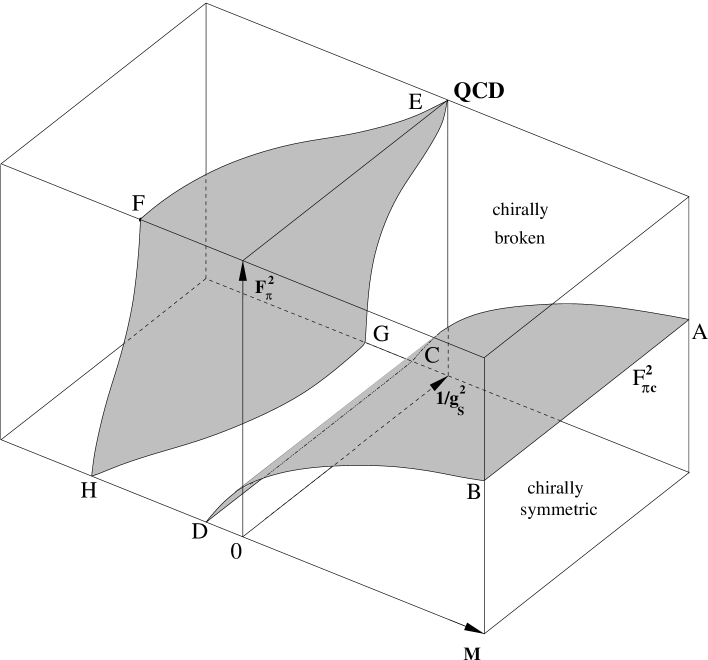
Figure 1: Possible form of the phase diagram of the chiral quark model in the $(M,F^{2}_{\pi},1/g_{s}^{2})$-space at $g_{A}=0$ and $r=1$. Structures behind the critical surface connecting the points $E$, $F$, $G$, and $H$ are not shown. The ranges of the variables are $M\in[-\infty,\infty]$ and $F_{\pi}^{2},1/g_{s}^{2}\in[0,\infty]$.

Next we consider the limit of infinite bare coupling $F_{\pi}^{2}=\infty$. The pion field $U_{x}=u_{x}^{2}$ is then frozen to a space-time independent constant $U_{0}$. Of course, this does not mean that $u_{x}$ is a constant. This can be illustrated as follows. If $U_{x}=U_{0}$ for all $x$, all $u_{x}$ can be diagonalized by the same unitary transformation $W$, i.e. $u_{x}=Wd_{x}W^{\dagger}$. The matrix $d_{x}=ds_{x}$ is a constant diagonal matrix $d\in U(1)^{N_{f}-1}$ up to a diagonal matrix $s_{x}\in{\sf Z\!\!\!Z}(2)^{N_{f}-1}$ obeying $s_{x}^{2}={\sf 1\!\!1}$. The Hermitean matrices $s_{x}$ have diagonal elements $\pm 1$ and determinant 1. Hence, we can now write

$$u_{x}=Wds_{x}W^{\dagger},$$ (7.1)

such that indeed $u_{x}^{2}=Wd^{2}W^{\dagger}=U_{0}$ is independent of $x$. Let us now consider the other fields in the $F_{\pi}^{2}=\infty$ limit. The lattice field $\tilde{V}_{x,\mu}$ takes the form

$$\tilde{V}_{x,\mu}=\frac{1}{2}[u_{x}^{\dagger}u_{x+\hat{\mu}}+u_{x}u_{x+\hat{\mu}}^{\dagger}]=Ws_{x}s_{x+\hat{\mu}}W^{\dagger}=V_{x,\mu}.$$ (7.2)

Since $\tilde{V}_{x,\mu}$ is already in $SU(N_{f})$, the $GL(N_{f})/SU(N_{f})$ coset decomposition yields $V_{x,\mu}=\tilde{V}_{x,\mu}$. Similarly, it is straightforward to show that $\tilde{A}_{x,\mu}=A_{x,\mu}^{L}=A_{x,\mu}^{R}=0$. We now perform the transformation $V_{x}=s_{x}W^{\dagger}$ on the constituent quark field

$$\Psi_{x}=V_{x}^{\dagger}\Psi_{x}^{\prime}=Ws_{x}\Psi_{x}^{\prime},\ \overline{\Psi}_{x}=\overline{\Psi}_{x}^{\prime}V_{x}=\overline{\Psi}_{x}s_{x}W^{\dagger}.$$ (7.3)

As a consequence,

$$\overline{\Psi}_{x}\Psi_{x}=\overline{\Psi}_{x}^{\prime}s_{x}W^{\dagger}Ws_{x}\Psi_{x}^{\prime}=\overline{\Psi}_{x}^{\prime}\Psi_{x}^{\prime},$$

$$\overline{\Psi}_{x}V_{x,\mu}\Psi_{x+\hat{\mu}}=\overline{\Psi}_{x}^{\prime}s_{x}W^{\dagger}Ws_{x}s_{x+\hat{\mu}}W^{\dagger}Ws_{x+\hat{\mu}}\Psi_{x+\hat{\mu}}^{\prime}=\overline{\Psi}_{x}^{\prime}\Psi_{x+\hat{\mu}}^{\prime},$$

$$\overline{\Psi}_{x+\hat{\mu}}V_{x,\mu}^{\dagger}\Psi_{x}=\overline{\Psi}_{x+\hat{\mu}}^{\prime}s_{x+\hat{\mu}}W^{\dagger}Ws_{x+\hat{\mu}}s_{x}W^{\dagger}Ws_{x}\Psi_{x}^{\prime}=\overline{\Psi}_{x+\hat{\mu}}^{\prime}\Psi_{x}^{\prime},$$ (7.4)

so that (for $F_{\pi}^{2}=\infty$) the action (6.4) takes the form

$$S[\overline{\Psi}^{\prime},\Psi^{\prime},G] = M\sum_{x}\overline{\Psi}_{x}^{\prime}\Psi_{x}^{\prime}+\frac{1}{2}\sum_{x,\mu}(\overline{\Psi}_{x}^{\prime}\gamma_{\mu}G_{x,\mu}\Psi_{x+\hat{\mu}}^{\prime}-\overline{\Psi}_{x+\hat{\mu}}^{\prime}\gamma_{\mu}G_{x,\mu}^{\dagger}\Psi_{x}^{\prime})$$

$$+ \frac{r}{2}\sum_{x,\mu}(2\overline{\Psi}_{x}^{\prime}\Psi_{x}^{\prime}-\overline{\Psi}_{x}^{\prime}G_{x,\mu}\Psi_{x+\hat{\mu}}^{\prime}-\overline{\Psi}_{x+\hat{\mu}}^{\prime}G_{x,\mu}^{\dagger}\Psi_{x}^{\prime})$$

$$- \frac{1}{g_{s}^{2}}\sum_{x,\mu,\nu}\mbox{Tr}[G_{x,\mu}G_{x+\hat{\mu},\nu}G_{x+\hat{\nu},\mu}^{\dagger}G_{x,\nu}^{\dagger}+G_{x,\nu}G_{x+\hat{\nu},\mu}G_{x+\hat{\mu},\nu}^{\dagger}G_{x,\mu}^{\dagger}].$$

(7.5)

Remarkably, this is nothing but the standard Wilson fermion action. Hence, in the limit $F_{\pi}^{2}=\infty$, $g_{s}\rightarrow 0$, and $M\rightarrow 0$ (point $E$ in fig. 1), we reach the usual continuum limit of lattice QCD. This point is connected to the point $F$ at strong coupling ($g_{s}=\infty$) by a line of second order phase transitions. Fine-tuning to this line, a massless “pion” emerges as a quark-antiquark bound state. This “pion” is not the Goldstone boson that results from chiral symmetry breaking, except in the continuum limit. Still, in Wilson’s approach to lattice QCD this particle represents the physical pion. Then, recovering chiral symmetry requires fine-tuning as well as taking the continuum limit. Of course, in the chiral quark model with a nonlinearly realized chiral symmetry, there is a genuine Goldstone pion. However, this particle decouples at $F_{\pi}^{2}=\infty$. It is tempting to try to avoid fine-tuning and to represent the physical pion by the Goldstone boson of the nonlinearly realized chiral symmetry. This would suggest to approach the QCD point $E$ from finite values of $F_{\pi}^{2}$ out of the chirally broken phase. As one approaches the point $E$, one should then avoid the critical surface connecting the points $E$, $F$, $G$, and $H$ because otherwise one would double-count the pion. However, it is not clear if one will obtain a new approach to QCD in this way. For example, it is likely that the explicit Goldstone pion decouples and that the QCD pion must still be assembled as a quark-antiquark bound state.

Let us now consider the $g_{s}=0$ plane in the phase diagram. Then the gluon field is completely frozen to a pure gauge $G_{x,\mu}=g_{x}g_{x+\hat{\mu}}^{\dagger}$. It should be noted that the continuum limit of lattice QCD is taken by sending $g_{s}\rightarrow 0$ in a controlled way, not by simply putting $g_{s}=0$. In particular, at $g_{s}=0$ there is no gluon field and thus no confinement. In this case, we transform the fermion field as $\Psi_{x}=g_{x}\Psi_{x}^{\prime}$, $\overline{\Psi}_{x}=\overline{\Psi}_{x}^{\prime}g_{x}^{\dagger}$, so that

$$\overline{\Psi}_{x}\Psi_{x}=\overline{\Psi}_{x}^{\prime}g_{x}^{\dagger}g_{x}\Psi_{x}^{\prime}=\overline{\Psi}_{x}^{\prime}\Psi_{x}^{\prime},$$

$$\overline{\Psi}_{x}G_{x,\mu}\Psi_{x+\hat{\mu}}=\overline{\Psi}_{x}^{\prime}g_{x}^{\dagger}g_{x}g_{x+\hat{\mu}}^{\dagger}g_{x+\hat{\mu}}\Psi_{x+\hat{\mu}}^{\prime}=\overline{\Psi}_{x}^{\prime}\Psi_{x+\hat{\mu}}^{\prime},$$

$$\overline{\Psi}_{x+\hat{\mu}}G_{x,\mu}^{\dagger}\Psi_{x}=\overline{\Psi}_{x+\hat{\mu}}^{\prime}g_{x+\hat{\mu}}^{\dagger}g_{x+\hat{\mu}}g_{x}^{\dagger}g_{x}\Psi_{x}^{\prime}=\overline{\Psi}_{x+\hat{\mu}}^{\prime}\Psi_{x}^{\prime}.$$ (7.6)

Hence, for $g_{s}=0$ the action (6.4) reduces to

$$S[\overline{\Psi}^{\prime},\Psi^{\prime},U] = M\sum_{x}\overline{\Psi}_{x}^{\prime}\Psi_{x}^{\prime}+\frac{1}{2}\sum_{x,\mu}(\overline{\Psi}_{x}^{\prime}\gamma_{\mu}V_{x,\mu}\Psi_{x+\hat{\mu}}^{\prime}-\overline{\Psi}_{x+\hat{\mu}}^{\prime}\gamma_{\mu}V_{x,\mu}^{\dagger}\Psi_{x}^{\prime})$$

$$+ \frac{ig_{A}}{2}\sum_{x,\mu}(\overline{\Psi}_{x}^{\prime}\gamma_{\mu}\gamma_{5}A^{L}_{x,\mu}\Psi_{x}^{\prime}+\overline{\Psi}_{x+\hat{\mu}}^{\prime}\gamma_{\mu}\gamma_{5}A^{R}_{x,\mu}\Psi_{x+\hat{\mu}}^{\prime})$$

$$+ \frac{r}{2}\sum_{x,\mu}(2\overline{\Psi}_{x}^{\prime}\Psi_{x}^{\prime}-\overline{\Psi}_{x}^{\prime}V_{x,\mu}\Psi_{x+\hat{\mu}}^{\prime}-\overline{\Psi}_{x+\hat{\mu}}^{\prime}V_{x,\mu}^{\dagger}\Psi_{x}^{\prime})$$

$$- \frac{F_{\pi}^{2}}{4}\sum_{x,\mu}\mbox{Tr}[U_{x}^{\dagger}U_{x+\hat{\mu}}+U_{x+\hat{\mu}}^{\dagger}U_{x}]-\frac{\langle\overline{\psi}\psi\rangle}{2}\sum_{x}\mbox{Tr}[{\cal M}U_{x}^{\dagger}+{\cal M}^{\dagger}U_{x}],$$

(7.7)

which has exactly the same form as the baryon action (3). Of course, here the field $\Psi_{x}$ describes a colored constituent quark. Since we have now switched off the strong interactions, these quarks are no longer confined.

Figure 2: Possible form of the phase diagram of the chiral quark model in the $(M,F_{\pi}^{2})$-plane at $g_{s}=0$, $g_{A}=0$, and $r=1$. The ranges of the variables are $M,F_{\pi}^{2}\in[-\infty,\infty]$.

For $N_{f}=2$, a possible form of the phase diagram in the $(M,F_{\pi}^{2})$-plane (at $g_{s}=0$) is depicted in fig. 2. It also includes the Aoki phase not shown in fig. 1. In the limit of infinite constituent quark mass, $M=\pm\infty$, the model reduces to an $SU(2)_{L}\otimes SU(2)_{R}=O(4)$ nonlinear $\sigma$-model for the pions. For $F_{\pi}^{2}>F_{\pi c}^{2}$, the pion field $U_{x}$ is ordered and hence chiral symmetry is spontaneously broken to $SU(2)_{L=R}=O(3)$, while for $F_{\pi}^{2}<F_{\pi c}^{2}$, it is restored. It is interesting to consider negative values of $F_{\pi}^{2}$ as well (still keeping $M=\pm\infty$). On a bi-partite lattice one can map the theory back to the one with positive values of $F_{\pi}^{2}$ by changing the sign of $U_{x}$ on all odd lattice sites. Hence, for $F_{\pi}^{2}<-F_{\pi c}^{2}$, there is an “antiferromagnetically” ordered phase in which chiral symmetry is again broken from $O(4)$ to $O(3)$. Hence, for $M=\pm\infty$, there are two phase transitions, one at $F_{\pi c}^{2}$ separating the usual “ferromagnetic” chirally broken from the “paramagnetic” chirally symmetric phase and another one at $-F_{\pi c}^{2}$ separating the “paramagnetic” from the “antiferromagnetic” broken phase.

At $M=0$ and $F_{\pi}^{2}=\infty$ (point $E$ in figs. 1 and 2) there is a second order phase transition at which the constituent quark mass vanishes. In addition, there are unphysical second order phase transitions at $M+2nr=0$ (with $n\in\{1,2,3,4\}$) at which some of the doubler fermions become massless. In the context of Wilson’s lattice QCD the region of $M<0$ was explored by Aoki [61]. He identified a rich structure including a phase in which parity and flavor are spontaneously broken. It should be noted that for $g_{A}=0$ the model (7) has a symmetry under the replacement of $M$ by $-(M+4r)$. This replacement can be compensated for by changing the sign of $\Psi_{x}$ on all even sites and the sign of $\overline{\Psi}_{x}$ on all odd sites. This symmetry manifests itself in the phase diagram of fig. 2. Our sketch of the Aoki phase in fig. 2 is inspired by its form in Wilson’s lattice QCD. The precise structure of the phase diagram can only be inferred from numerical simulations. The phase diagram of fig. 2 is a possible interpolation between the limits $M=\pm\infty$ and $F_{\pi}^{2}=\infty$, partly inspired by the phase diagram of the Smit-Swift model and other related Higgs-Yukawa models [62, 63, 64]. Attempts to construct chiral gauge theories as the continuum limit of such lattice models have failed because it was impossible to remove the doubler fermions, both at weak and at strong Yukawa couplings [65]. Such problems do not affect our construction of lattice effective theories with nonlinearly realized chiral symmetry because, in that case, there is no need to approach a second order phase transition to extract low-energy continuum physics. However, attempts to construct full QCD with a manifest nonlinearly realized chiral symmetry on the lattice are likely to fail for the same reasons as the Smit-Swift model did. Still, it is interesting to ask if the lattice chiral symmetry of Ginsparg-Wilson fermions can be realized nonlinearly. We leave such questions for future investigations.

8 Conclusions

In this paper we have constructed lattice theories with baryon or constituent quark fields on which chiral symmetry is nonlinearly realized. In this framework the fermion doublers are removed by the Wilson term without breaking chiral symmetry explicitly. This is possible because fermion fields do not contribute to anomalies in theories with nonlinearly realized chiral symmetries. Instead the anomalies must be included explicitly in the form of Wess-Zumino-Witten and Goldstone-Wilczek terms. The lattice construction of such terms remains an interesting challenge for future investigations.

The use of nonlinearly realized chiral symmetry is well established in the context of chiral perturbation theory which provides a power counting scheme for a systematic low-energy expansion. However, also non-perturbative problems may arise in the low-energy regime. Some of these problems can be dealt with analytically [28]. In general, however, such problems require some numerical work. While one can still proceed without Monte Carlo methods in investigations of few-nucleon systems [30, 31], this is likely to change as one moves on to larger nuclei and ultimately to nuclear matter [32]. Our lattice formulation provides a framework in which future numerical studies of this kind can be performed on a solid theoretical basis.

Even if one leaves the framework of a systematic low-energy expansion, the nonlinear realization of chiral symmetry on the lattice may provide insight into interesting physical questions. For example, as we have seen, in a model of static baryons at non-zero chemical potential one can investigate universal aspects of the QCD phase diagram, like the nature of the critical endpoint of the chiral phase transition line. In the static baryon approximation, one cannot expect to obtain results directly relevant to QCD for non-universal quantities such as the location of the critical endpoint. Still, one may be able to collect, for example, qualitative information on how the critical endpoint moves as the strange quark mass is varied.

Another interesting example is the chiral quark model of Georgi and Manohar. It holds the promise to explain the success of the non-relativistic quark model and has successfully described a variety of physical properties of hadrons. However, there is a number of potential dynamical problems that can only be addressed non-perturbatively. Our lattice formulation allows us to investigate if these potential dynamical problems do arise or not. In particular, the confinement of constituent quarks — out of reach of conventional methods — can be directly addressed with lattice methods. These investigations will allow one to decide if the chiral quark model indeed provides a satisfactory explanation for the success of the non-relativistic quark model. Along the way, one will be able to sharpen the algorithmic tools of dynamical fermion simulations in a model that shares many features with QCD — most important a manifest chiral symmetry — but which should be much simpler to simulate than Ginsparg-Wilson fermions in the chiral limit.

At this stage, it is not clear if lattice theories with a nonlinearly realized chiral symmetry can also provide a formulation of full QCD beyond low-energy effective theories. In order to answer this question, one may attempt to relate lattice QCD with Ginsparg-Wilson fermions to a lattice theory with explicit pion fields and a nonlinearly realized chiral symmetry. If such a connection can be found analytically, one would expect that the anomalies of Ginsparg-Wilson fermions manifest themselves as Wess-Zumino-Witten and Goldstone-Wilczek terms of the lattice pion field. This is an interesting project for future studies which holds the promise to further deepen our understanding of the non-perturbative regularization of chiral symmetry.

References

- [1] K. G. Wilson, in “New Phenomena in Subnuclear Physics,” Erice Lectures 1975, edited by A. Zichichi (Plenum, New York, 1977).
- [2] H. B. Nielsen and M. Ninomiya, Phys. Lett. B105 (1981) 219; Nucl. Phys. B185 (1981) 20 [Erratum-ibid. B195 (1982) 541]; ibid. B193 (1981) 173.
- [3] D. Friedan, Commun. Math. Phys. 85 (1982) 481.
- [4] D. B. Kaplan, Phys. Lett. B288 (1992) 342; Nucl. Phys. B (Proc. Suppl.) 30 (1993) 597.
- [5] R. Narayanan and H. Neuberger, Phys. Lett. B302 (1993) 62; Nucl. Phys. B443 (1995) 305.
- [6] P. H. Ginsparg and K. G. Wilson, Phys. Rev. D25 (1982) 2649.
- [7] P. Hasenfratz, Nucl. Phys. B (Proc. Suppl.) 63 (1998) 53.
- [8] H. Neuberger, Phys. Rev. D57 (1998) 5417.
- [9] M. Lüscher, Phys. Lett. B428 (1998) 342.
- [10] M. Lüscher, Nucl. Phys. B549 (1999) 295; Nucl. Phys. B568 (2000) 162.
- [11] J. Goldstone, Nuovo Cim. 19 (1961) 154.
- [12] S. Weinberg, Phys. Rev. Lett. 18 (1967) 188; Phys. Rev. 166 (1968) 1568.
- [13] S. Coleman, J. Wess, and B. Zumino, Phys. Rev. 177 (1969) 2239.
- [14] C. G. Callan, S. Coleman, J. Wess, and B. Zumino, Phys. Rev. 177 (1969) 2247.
- [15] S. Weinberg, Physica 96A (1979) 327.
- [16] J. Gasser and H. Leutwyler, Ann. Phys. 158 (1984) 142; Nucl. Phys. B250 (1985) 465.
- [17] H. Georgi, Weak Interactions and Modern Particle Theory (Benjamin/Cummings, Menlo Park CA, 1984).
- [18] J. Gasser, M. E. Sainio, and A. Svarc, Nucl. Phys. B307 (1988) 779.
- [19] E. Jenkins and A. Manohar, Phys. Lett. B255 (1991) 558.
- [20] V. Bernard, N. Kaiser, J. Kambor, and U.-G. Meissner, Nucl. Phys. B388 (1992) 315.
- [21] T. Becher and H. Leutwyler, Eur. Phys. J. C9 (1999) 643.
- [22] P. Hasenfratz and F. Niedermayer, Z. Phys. B92 (1993) 91.
- [23] I. A. Shushpanov and A. V. Smilga, Phys. Rev. D59 (1999) 054013.
- [24] R. Lewis and P.-P. A. Ouimet, Phys. Rev. D64 (2001) 034005.
- [25] A. S. Kronfeld, “Uses of effective field theory in lattice QCD,” hep-lat/0205021. (To appear in “At the Frontiers of Particle Physics: Handbook of QCD,” Vol. 4, edited by M. Shifman.)
- [26] S. Myint and C. Rebbi, Nucl. Phys. B421 (1994) 241.
- [27] A. R. Levi, V. Lubicz, and C. Rebbi, Phys. Rev. D56 (1997) 1101.
- [28] H. Leutwyler, Phys. Lett. B189 (1987) 197.
- [29] D. B. Kaplan, M. J. Savage, and M. B. Wise, Phys. Lett. B424 (1998) 390; Nucl. Phys. B534 (1998) 329.
- [30] P. F. Bedaque, H.-W. Hammer, and U. van Kolck, Phys. Rev. C58 (1998) 641; Nucl. Phys. A676 (2000) 357.
- [31] P. F. Bedaque and U. van Kolck, Ann. Rev. Nucl. Part. Sci. 52 (2002) 339.
- [32] H.-M. Müller, S. E. Koonin, R. Seki, and U. van Kolck, Phys. Rev. C61 (2000) 044320.
- [33] J. Wess and B. Zumino, Phys. Lett. 37B (1971) 95.
- [34] E. Witten, Nucl. Phys. B223 (1983) 422; Nucl. Phys. B223 (1983) 433.
- [35] J. Goldstone and F. Wilczek, Phys. Rev. Lett. 47 (1981) 986.
- [36] H. Georgi and A. Manohar, Nucl. Phys. B234 (1984) 189.
-
[37]
R. C. Brower, Y. Shen, and C.-I. Tan, Nucl. Phys. B (Proc. Suppl.) 34 (1994)
210;
R. C. Brower, K. Orginos, and C.-I. Tan, Nucl. Phys. B (Proc. Suppl.) 42 (1995) 42. -
[38]
J. B. Kogut, J.-F. Lagae, and D. K. Sinclair, Phys. Rev. D58 (1998) 034504;
J. B. Kogut and D. K. Sinclair, Phys. Lett. B492 (2000) 228; Phys. Rev. D64 (2001) 034508. - [39] A. Borici and P. de Forcrand, Nucl. Phys. B454 (1995) 645.
- [40] C. Alexandrou et al., Phys. Rev. D60 (1999) 034504.
- [41] T. Takaishi and P. de Forcrand, Nucl. Phys. B (Proc. Suppl.) 94 (2001) 818.
- [42] S. Aoki et al., Phys. Rev. D65 (2002) 094507.
- [43] G. ’t Hooft, Phys. Rev. Lett. 37 (1976) 8; Phys. Rev. D14 (1976) 3432 [Erratum-ibid. D18 (1978) 2199].
- [44] E. Witten, Nucl. Phys. B156 (1979) 269.
- [45] G. Veneziano, Nucl. Phys. B159 (1979) 213.
- [46] E. Witten, Phys. Lett. 117B (1982) 324.
- [47] E. D’Hoker and E. Farhi, Phys. Lett. B134 (1984) 86.
- [48] T. Skyrme, Proc. Roy. Soc. A260 (1961) 127; Nucl. Phys. 31 (1962) 556.
- [49] O. Bär and U.-J. Wiese, Nucl. Phys. B609 (2001) 225.
- [50] T. D. Lee and C. N. Yang, Nuovo Cim. 10 (1956) 749.
- [51] A. Manohar and G. W. Moore, Nucl. Phys. B243 (1984) 55.
- [52] I. Bender et al., Nucl. Phys. B (Proc. Suppl.) 26 (1992) 323.
- [53] T. C. Blum, J. E. Hetrick, and D. Toussaint, Phys. Rev. Lett. 76 (1996) 1019.
- [54] J. Engels, O. Kaczmarek, F. Karsch, and E. Laermann, Nucl. Phys. B558 (1999) 307; Nucl. Phys. B (Proc. Suppl.) 83 (2000) 369.
- [55] M. Alford, S. Chandrasekharan, J. Cox, and U.-J. Wiese, Nucl. Phys. B602 (2001) 61.
- [56] M. Stephanov, K. Rajagopal, and E. Shuryak, Phys. Rev. Lett. 81 (1998) 4816; Phys. Rev. D60 (1999) 114028.
- [57] Z. Fodor and S. D. Katz, JHEP 0203 (2002) 014.
- [58] C. R. Allton et al., Phys. Rev. D66 (2002) 074507.
- [59] P. de Forcrand and O. Philipsen, Nucl. Phys. B642 (2002) 290.
- [60] M. E. Peskin, Nucl. Phys. B175 (1980) 197.
- [61] S. Aoki, Phys. Rev. D30 (1984) 2653; Phys. Rev. D33 (1986) 2399; Phys. Rev. D34 (1986) 3170; Phys. Rev. Lett. 57 (1986) 3136.
- [62] J. Smit, Nucl. Phys. B175 (1980) 307; Acta Phys. Polon. B17 (1986) 531.
- [63] P. V. D. Swift, Phys. Lett. B145 (1984) 256.
- [64] W. Bock et al., Nucl. Phys. B344 (1990) 207.
- [65] D. N. Petcher, Nucl. Phys. B (Proc. Suppl.) 30 (1993) 50.