Monte Carlo errors with less errors.

Abstract

We explain in detail how to estimate mean values and assess statistical errors for arbitrary functions of elementary observables in Monte Carlo simulations. The method is to estimate and sum the relevant autocorrelation functions, which is argued to produce more certain error estimates than binning techniques and hence to help toward a better exploitation of expensive simulations. An effective integrated autocorrelation time is computed which is suitable to benchmark efficiencies of simulation algorithms with regard to specific observables of interest. A Matlab code is offered for download that implements the method. It can also combine independent runs (replica) allowing to judge their consistency.

HU-EP-03/32

SFB/CCP-03-12

1 Formulation of the problem

In this article we collect some theory and formulas for the practical estimation of statistical and systematic errors in Monte Carlo simulations. Emphasis is put on the estimation of in general nonlinear functions (‘derived quantities’) of the primary expectation values. The strategy focuses on the explicit determination of the relevant autocorrelation functions and times. We shall discuss why this is advantageous compared to the popular binning techniques, which handle autocorrelations only implicitly. A Matlab code is made available, which implements the method described here.

The material given here is only partially new. It has been briefly discussed in the appendix of [1] and in internal notes of the ALPHA collaboration [2] and in lecture notes [3]. However, due to the fact that mastering this topic is an indispensable prerequisite for every student or researcher in the popular field of lattice simulation, we felt that there is a gap in the readily citeable literature which we want to fill here.

We assume to have a number of primary observables enumerated by a Greek index with exact statistical mean values $A_{\alpha}$. The object to be estimated is a function of these,

$$F\equiv f(A_{1},A_{2},\ldots)\equiv f(A_{\alpha}).$$ (1)

A typical example is given by reweighting, where a quotient $F=A_{1}/A_{2}$ has to be determined. A more involved case are fit-parameters determined by correlation functions over a range of separations.

For the estimation we employ Monte Carlo estimates of the primary observables given by $a_{\alpha}^{i}$. For each observable there are $i=1,2,\ldots,N$ successive estimates separated by executions of some valid update procedure. We assume that the Markov chain has been equilibrated before recording data beginning with $i=1$. This has to be secured from case to case, and we in particular recommend visual inspections of initial histories of observables to decide on safely discarding data. A posteriori one should also check that the equilibration time was much longer than autocorrelation times found in the analysis of the supposed equilibrium data.

A key theoretical quantity for error estimation is the autocorrelation [4, 5] function $\Gamma_{\alpha\beta}$ defined by

$$\left\langle(a_{\alpha}^{i}-A_{\alpha})(a_{\beta}^{i+n}-A_{\beta})\right\rangle=\Gamma_{\alpha\beta}(n).$$ (2)

that correlates the deviation of the $i$’th estimate for $A_{\alpha}$ with the deviation for variable $\beta$ after performing $n\geq 0$ updates. Averages $\langle\,\cdot\,\rangle$ here and throughout this paper refer to an ensemble of identical numerical experiments with independent random numbers and initial states — a concept useful for errors that are themselves statistical in nature. The dependence of $\Gamma_{\alpha\beta}$ on the separation $n$ alone is due to being in equilibrium.

We take the simulation to produce configurations $\phi_{i}$ distributed with the normalized Boltzmannian $P(\phi)$. The update algorithm is specified by transition probabilities $W(\phi\to\phi^{\prime})$ and the measurements by $a_{\alpha}^{i}={\cal O}_{\alpha}(\phi_{i})$. Then the autocorrelation function in equilibrium is given as a double sum over configurations,

$$\Gamma_{\alpha\beta}(n)=\sum_{\phi}\sum_{\phi^{\prime}}P(\phi)W^{n}(\phi\to\phi^{\prime})({\cal O}_{\alpha}(\phi)-A_{\alpha})({\cal O}_{\beta}(\phi^{\prime})-A_{\beta}).$$ (3)

Here $W^{n}$ characterizes transitions by a succession of $n$ update steps. If $W$ obeyed detailed balance with respect to $P$, we would conclude symmetry in the indices $\alpha\beta$. In practice we usually have only stability and no such symmetry seems to be implied in general. It is however natural and useful to define

$$\Gamma_{\alpha\beta}(-n)=\Gamma_{\beta\alpha}(n)$$ (4)

implying a combined symmetry. Obviously $\Gamma_{\alpha\beta}(0)$ is the symmetric covariance matrix with the ordinary variances on the diagonal. It is a (static) property of the simulated statistical system alone, while $\Gamma$-values for nonzero separation are dynamic and depend on the Monte Carlo algorithm in use.

We end this theoretical setup by a slight generalization of our analysis. We add another index to the estimates of the primary observables, $a_{\alpha}^{i,r}$. The index $r=1,2,\ldots,R$ counts a number of statistically independent replica. These are independent simulations which typically arise from repeated runs, or in particular, if parallel computers are used in the ‘trivial parallelization’ mode. For each replicum $r$ there are $i=1,2,\ldots,N_{r}$ successive equilibrium estimates separated by executions of the same update procedure. Obviously (2) becomes

$$\left\langle(a_{\alpha}^{i,r}-A_{\alpha})(a_{\beta}^{j,s}-A_{\beta})\right\rangle=\delta_{rs}\Gamma_{\alpha\beta}(j-i).$$ (5)

2 Errors and biases

2.1 Primary observables

We define the per replicum means

$$\bar{a}_{\alpha}^{r}=\frac{1}{N_{r}}\sum_{i=1}^{N_{r}}\;a_{\alpha}^{i,r}.$$ (6)

and in terms of them the natural estimator for the primary quantities $A_{\alpha}$

$$\bar{\bar{a}}_{\alpha}=\frac{1}{N}\sum_{r=1}^{R}\;N_{r}\,\bar{a}_{\alpha}^{r}$$ (7)

with the total number of estimates

$$N=\sum_{r=1}^{R}N_{r}\,.$$ (8)

Introducing the deviations

$$\bar{\delta}_{\alpha}^{r}=\bar{a}_{\alpha}^{r}-A_{\alpha}\,,\quad\bar{\bar{\delta}}_{\alpha}=\bar{\bar{a}}_{\alpha}-A_{\alpha}\,.$$ (9)

we state that these estimators are unbiased,

$$\langle\bar{\delta}_{\alpha}^{r}\rangle=0=\langle\bar{\bar{\delta}}_{\alpha}\rangle.$$ (10)

We assume a normal distribution which is then completely defined by the covariance matrix given by

$$\langle\;\bar{\delta}_{\alpha}^{r}\,\bar{\delta}_{\beta}^{s}\;\rangle=\frac{1}{N_{r}^{2}}\sum_{i,j=1}^{N_{r}}\Gamma_{\alpha\beta}(j-i)\delta_{rs}=\frac{1}{N_{r}}C_{\alpha\beta}\,\delta_{rs}\times(1+\mbox{\rm O}(\tau/N_{r}))\,$$ (11)

where

$$C_{\alpha\beta}=\sum_{t=-\infty}^{\infty}\Gamma_{\alpha\beta}(t)$$ (12)

does not depend on the run-length. Here and in the following it is assumed that a finite scale $\tau$ characterizes the asymptotic exponential decay of $\Gamma_{\alpha\beta}$ with $|t|$. The claimed $N_{r}$-dependence holds for runs with lengths $N_{r}\gg\tau$ and if this condition is violated, an error estimation is hardly possible. For the covariance matrix of $\bar{\bar{a}}_{\alpha}$

$$\langle\;\bar{\bar{\delta}}_{\alpha}\,\bar{\bar{\delta}}_{\beta}\;\rangle=\frac{1}{N}C_{\alpha\beta}\times(1+\mbox{\rm O}(R\tau/N))$$ (13)

follows. Roughly speaking, as expected, $\bar{\bar{a}}_{\alpha}$ differs from $A_{\alpha}$ by an error of order $1/\sqrt{N}$ and the task of an error analysis amounts to a reasonably accurate estimation of $C_{\alpha\beta}$ which includes all autocorrelation effects.

2.2 Derived quantities

To determine $F$ we consider estimators

$$\bar{\bar{F}}=f(\bar{\bar{a}}_{\alpha})$$ (14)

and

$$\bar{F}=\frac{1}{N}\sum_{r=1}^{R}\,N_{r}\,f(\bar{a}_{\alpha}^{r}).$$ (15)

We assume the estimates of the primary observables to be accurate enough to justify Taylor expansions of $f$ in the fluctuations, for example

$$\bar{\bar{F}}=F+\sum_{\alpha}f_{\alpha}\bar{\bar{\delta}}_{\alpha}+\frac{1}{2}\sum_{\alpha\beta}f_{\alpha\beta}\,\bar{\bar{\delta}}_{\alpha}\bar{\bar{\delta}}_{\beta}+\dots$$ (16)

with derivatives

$$f_{\alpha}=\frac{\partial f}{\partial A_{\alpha}},\quad f_{\alpha\beta}=\frac{\partial^{2}f}{\partial A_{\alpha}\partial A_{\beta}}$$ (17)

taken at the exact values $A_{1},A_{2},\ldots$. It follows that our estimators for $F$ are biased unless $f$ is linear,

$$\langle\bar{\bar{F}}-F\rangle\simeq\frac{1}{2N}\sum_{\alpha\beta}f_{\alpha\beta}\,C_{\alpha\beta}\simeq\frac{1}{R}\,\langle\bar{F}-F\rangle\,,$$ (18)

Usually, this bias is negligible compared to statistical errors due to large enough $N$. Replica ($R\geq 2$) can however be used to control and, if deemed to be appropriate, cancel the leading bias by using

$$\langle\bar{\bar{F}}-F\rangle\simeq\frac{1}{R-1}\,\langle\bar{F}-\bar{\bar{F}}\rangle$$ (19)

to replace

$$\bar{\bar{F}}\to\frac{R\bar{\bar{F}}-\bar{F}}{R-1}\,.$$ (20)

The error $\sigma_{F}$ is to leading order given by

$$\sigma_{F}^{2}=\langle\,(\bar{\bar{F}}-F)^{2}\,\rangle\simeq\frac{1}{N}C_{F}$$ (21)

with

$$C_{F}=\sum_{\alpha\beta}f_{\alpha}f_{\beta}\,C_{\alpha\beta}\,.$$ (22)

We rewrite this expression as

$$\sigma_{F}^{2}=\frac{2\tau_{{\rm int},F}}{N}\,v_{F}$$ (23)

with the effective ‘naive’ – i.e. disregarding autocorrelations – variance relevant for $F$

$$v_{F}=\sum_{\alpha\beta}f_{\alpha}f_{\beta}\Gamma_{\alpha\beta}(0)$$ (24)

and the integrated autocorrelation time for $F$

$$\tau_{{\rm int},F}=\frac{1}{2v_{F}}\sum_{t=-\infty}^{\infty}\sum_{\alpha\beta}f_{\alpha}f_{\beta}\Gamma_{\alpha\beta}(t).$$ (25)

This one number encodes the efficiency of the algorithm in use for a determination of $F$, if its execution time per update is known. To appreciate this notation for the ratio of the true to the naive error two extremal cases are instructive. In the absence of autocorrelations, $\Gamma_{\alpha\beta}(t)\propto\delta_{t,0}$, we have $2\tau_{{\rm int},F}=1$ and (23) is the standard error. For a purely exponential behaviour, $\Gamma_{\alpha\beta}(t)\propto\exp(-|t|/\tau)$, this scale is recovered, $\tau_{{\rm int},F}=\tau+\mbox{\rm O}(\tau^{-1})$. In general there are however many contributions and $\tau_{{\rm int},F}$ is more like a ‘dynamical susceptibility’. Another interpretation of (23) is, that only the reduced number of $N/(2\tau_{{\rm int},F})$ estimates are effectively independent to bring down statistical errors.

If we have $R\geq 2$ replica another consistency check is useful. The replica estimates $f(\bar{a}_{\alpha}^{r})$ are assumed to be normally distributed. Their variances are

$$\left\langle\,\left(f(\bar{a}_{\alpha}^{r})-F\right)^{2}\,\right\rangle=\frac{C_{F}}{N_{r}}.$$ (26)

We may imagine to do a $\chi^{2}$ fit of the replica estimates to a constant $K$ by minimizing

$$\chi^{2}(K)=\sum_{r}\frac{(f(\bar{a}_{\alpha}^{r})-K)^{2}}{C_{F}/N_{r}}.$$ (27)

The minimum occurs precisely at $K=\bar{F}$ given in (15). The probability to find in such a ‘fit’ a minimal $\chi^{2}\geq x$ is given by

$$Q=1-P(x/2,(R-1)/2),$$ (28)

where $P$ is the incomplete Gamma function,

$$P(U,n)=\frac{1}{\Gamma(n)}\int_{0}^{U}du\,u^{n-1}\,\exp(-u).$$ (29)

Taking the actually observed $x=\chi^{2}(\bar{F})$ we obtain the so-called goodness of fit. It is very unlikely to see $Q$-values much less than 0.1, if the underlying distribution has the required properties, and this is hence a good consistency check [6]. In a histogram plot we may in addition inspect

$$p_{r}=\frac{f(\bar{a}_{\alpha}^{r})-\bar{F}}{\sigma_{F}\sqrt{N/N_{r}-1}}$$ (30)

which should have zero mean and unit variance.

In the next section we develop numerical estimators for $v_{F}$ and $\tau_{{\rm int},F}$, which at present are not yet of practical use, since they so far involve the numerically unknown exact $A_{\alpha}$ and $\Gamma_{\alpha\beta}$.

3 Extraction of errors from measured data

3.1 Error estimators

We now describe what we would like to call the $\Gamma$-method of error estimation (as opposed to binning, see App.B), where we explicitly estimate the autocorrelation function.

In terms of the given estimates $a_{\alpha}^{i,r}$ we define an estimator $\bar{\bar{\Gamma}}_{\alpha\beta}$ of the autocorrelation function

$$\bar{\bar{\Gamma}}_{\alpha\beta}(t)=\frac{1}{N-Rt}\sum_{r=1}^{R}\sum_{i=1}^{N_{r}-t}(a_{\alpha}^{i,r}-\bar{\bar{a}}_{\alpha})(a_{\beta}^{i+t,r}-\bar{\bar{a}}_{\beta})$$ (31)

where $0\leq t\ll N_{r}$ for all $r$ is understood. An important principle underlying this choice is to avoid unnecessary noise from terms which vanish (only) on average. Therefore the correlation is first taken within each replicum and only then averaged. Using arguments of the same type as for (11) the leading bias of this estimator is evaluated,

$$\langle\,\bar{\bar{\Gamma}}_{\alpha\beta}(t)\,\rangle-\Gamma_{\alpha\beta}(t)\approx-\frac{C_{\alpha\beta}}{N}.$$ (32)

It comes from subtracting in (31) the ensemble mean instead of the exact average. For uncorrelated data this is the well known bias in the estimator of the variance cancelled by the $N-1$ instead of $N$ normalization. For the moment we neglect this bias of order $1/N$ relative to the $1/\sqrt{N}$ statistical error in $\bar{\bar{\Gamma}}_{\alpha\beta}$ to be worked out in the next subsection, and come back to it later.

For the derived quantity $F$ only the projected autocorrelation is required,

$$\bar{\bar{\Gamma}}_{F}(t)=\sum_{\alpha\beta}\bar{\bar{f}}_{\alpha}\bar{\bar{f}}_{\beta}\bar{\bar{\Gamma}}_{\alpha\beta}(t)$$ (33)

where $\bar{\bar{f}}_{\alpha}$ is the gradient as in (17) but now evaluated at arguments $\bar{\bar{a}}_{1},\bar{\bar{a}}_{2},\ldots$, which inflicts a small relative error of order $1/N$ that we do not attempt to cancel.

As practical estimators for $v_{F}$ and $C_{F}$ we take

$$\bar{\bar{v}}_{F}=\bar{\bar{\Gamma}}_{F}(0)$$ (34)

and

$$\bar{\bar{C}}_{F}(W)=\left[\bar{\bar{\Gamma}}_{F}(0)+2\sum_{t=1}^{W}\bar{\bar{\Gamma}}_{F}(t)\right]\,.$$ (35)

A bias results from the truncation of the autocorrelation sum,

$$\frac{\langle\,\bar{\bar{C}}_{F}(W)\,\rangle-C_{F}}{C_{F}}\sim-\exp(-W/\tau).$$ (36)

For a purely exponential $\Gamma_{F}$ this is an approximate equality, otherwise an order of magnitude statement with the scale $\tau$ introduced at the end of section 2.1. The summation window $W$ has to be chosen with care. On the one hand it has to be large compared to the decay time $\tau$ for a small systematic error, on the other hand with too large $W$ one includes terms with negligible signal but excessive noise. In the next subsection we shall define an automatic procedure to choose $W$.

In a frequently met case we have many primary observables $A_{\alpha}$ but only want to estimate a few functions of them. Then it is advantageous to actually not compute the full autocorrelation matrices $\bar{\bar{\Gamma}}_{\alpha\beta}(t)$ but to just form $\bar{\bar{a}}_{\alpha}$ and $\bar{\bar{f}}_{\alpha}$ and immediately project the measured data

$$a_{\alpha}^{i,r}\to a_{f}^{i,r}=\sum_{\alpha}\bar{\bar{f}}_{\alpha}a_{\alpha}^{i,r}$$ (37)

to base the remaining autocorrelation analysis directly on them.

Another practical point concerns the computation of $\bar{\bar{f}}_{\alpha}$. It may well be inconvenient or even impossible to analytically specify the gradient of $f$ and we may prefer to evaluate it numerically based on the supplied routine for $f$ itself only. A natural scale $h_{\alpha}$ is extracted from the data,

$$h_{\alpha}=\sqrt{\frac{\bar{\bar{\Gamma}}_{\alpha\alpha}(0)}{N}}\;,$$ (38)

and we take

$$\bar{\bar{f}}_{\alpha}\approx\frac{1}{2h_{\alpha}}[f(\bar{\bar{a}}_{1},\bar{\bar{a}}_{2},\dots,\bar{\bar{a}}_{\alpha}+h_{\alpha},\dots)-f(\bar{\bar{a}}_{1},\bar{\bar{a}}_{2},\dots,\bar{\bar{a}}_{\alpha}-h_{\alpha},\dots)]$$ (39)

as a numerical estimate for the gradient of $f$ with negligible errors of $\mbox{\rm O}(h_{\alpha}^{2})\propto 1/N$.

3.2 Error of the error

When an error is assessed numerically in a Monte Carlo it is itself affected by statistical error. This is usually not quantified. But to rate algorithms on the basis of the $\tau_{{\rm int},F}$ they produce for physically interesting $F$ it is better to at least have a rough idea. This is even more true, if one wants to falsify a theoretical prediction based on one of these ‘$2.5\,\sigma$ discrepancies’, while maybe the estimate of $\sigma_{F}$ itself is uncertain by a factor 2.

In appendix A the very convenient approximate formula

$$\langle(\bar{\bar{C}}_{F}(W)-C_{F})^{2}\rangle\approx\frac{2(2W+1)}{N}C_{F}^{2}\,.$$ (40)

is derived that was to our knowledge first given in [4]. For the quotient

$$\bar{\bar{\tau}}_{{\rm int},F}(W)=\frac{\bar{\bar{C}}_{F}(W)}{2\bar{\bar{v}}_{F}}$$ (41)

we similarly find with the help of (57) and (58)

$$\langle(\bar{\bar{\tau}}_{{\rm int},F}(W)-\tau_{{\rm int},F})^{2}\rangle\approx\frac{4}{N}\,(W+1/2-\tau_{{\rm int},F})\tau_{{\rm int},F}^{2}.$$ (42)

Beside the statistical error of $\bar{\bar{C}}_{F}(W)$ there is the systematic error from the $W$-truncation in (36). We define as optimal the $W$ value that minimizes the sum of the absolute values of these errors and yields a total relative error

$$\frac{\delta_{\rm tot}(\bar{\bar{\sigma}}_{F})}{\bar{\bar{\sigma}}_{F}}\approx\frac{1}{2}\min_{W}\left(\exp(-W/\tau)+2\sqrt{W/N}\right)$$ (43)

for the final error estimate

$$\bar{\bar{\sigma}}_{F}^{2}=\frac{\bar{\bar{C}}(W)}{N}$$ (44)

evaluated at the optimal $W$. It is a function of $N/\tau$ and plotted in Fig.1

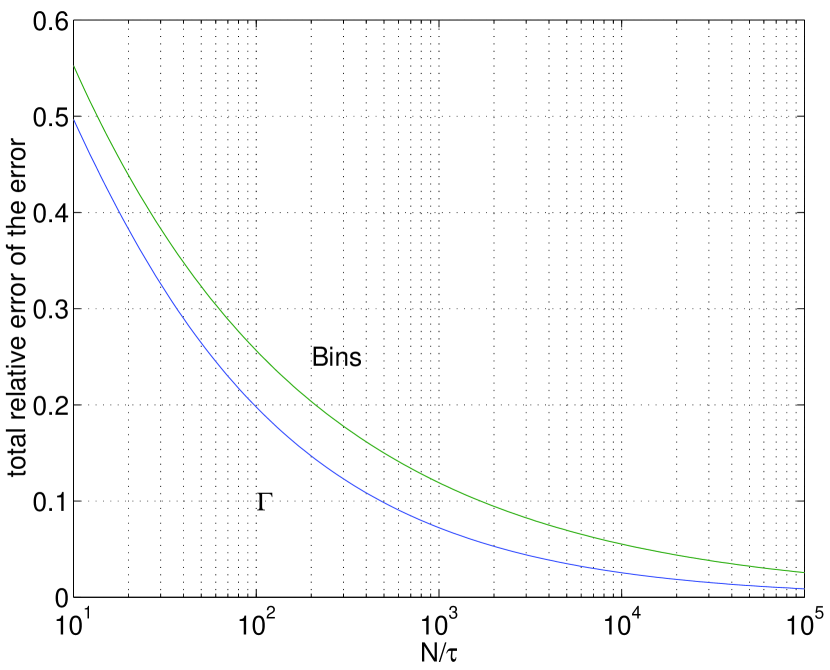
Figure 1: Relative total error of the error estimate for the $\Gamma$-method and for binning.

for relevant arguments. The minimum leads to a simple transcendental equation that we solved numerically, but it can also be well approximated by $W=\tau\ln(N/\tau)/2$. The asymptotic behaviour is $\delta_{\rm tot}\propto\sqrt{\ln(N)/N}$. Due to the exponential behaviour (36) the systematic component of the error becomes negligible at large N, albeit only slowly,

$$\frac{\delta_{\rm sys}(\bar{\bar{\sigma}}_{F})}{\delta_{\rm stat}(\bar{\bar{\sigma}}_{F})}=\frac{\tau}{2W}\approx\frac{1}{\ln(N/\tau)}\,.$$ (45)

A simple and popular alternative to the analysis method just described are binning methods, where data are pre-averaged over sections of the history of length $B$. These bin averages are taken as independent estimates. For both ordinary and jackknife binning (see appendix B for more details) a relative systematic error of the error estimate occurs, which decays only proportional to $\tau/B$. The relative statistical error of the error due to the finite number of bins is $\sqrt{2B/N}$. By balancing these errors similarly as before we find the total error at optimal bin size

$$\frac{\delta_{\rm tot}(\bar{\sigma}_{F{\,\rm bin}})}{\bar{\sigma}_{F{\,\rm bin}}}\approx\frac{1}{2}\min_{B}\left(\tau/B+\sqrt{2B/N}\right)=\frac{3}{2}(2N/\tau)^{-1/3}$$ (46)

which is reached for

$$B=\tau(2N/\tau)^{1/3}$$ (47)

and is also shown in Fig.1. Here the ratio of systematic to statistical error is constant,

$$\frac{\delta_{\rm sys}(\bar{\sigma}_{F{\,\rm bin}})}{\delta_{\rm stat}(\bar{\sigma}_{F{\,\rm bin}})}=\frac{1}{2}\,.$$ (48)

In comparing the $\Gamma$-method with binning it is clear now that the bin size $B$ and the window size $2W$ play a very similar role. All advantages of the $\Gamma$-method derive from the exponential in $W$ rather than inverse power in $B$ behaviour of the systematic error of the error. One could say, that in this way we have an improved estimator of the error whose own error decays with a (slightly) larger power of $N$.

We briefly come back to the bias in our error estimate caused by the right hand side of (32). Cancelling this term when estimating $C_{F}$ by (35) amounts to enlarging

$$\bar{\bar{C}}_{F}(W)\to\bar{\bar{C}}_{F}(W)\left(1+\frac{2W+1}{N}\right)\,,$$ (49)

which at the optimal $W$ value represents a correction down by a factor $1/\sqrt{N}$ (up to logs) relative to both contributions in (43). Since the correction is simple and known in closed form we include it in applications.

3.3 Automatic windowing procedure

We present now an algorithm to automatically choose $W$ that is similar but not identical to the one proposed in [4]. To determine $W$ in an actual data analysis, we start from a hypothesis that $\tau\sim S\tau_{{\rm int},F}$ with some factor $S$. More precisely, we solve

$$2\bar{\bar{\tau}}_{{\rm int},F}(W)=\sum_{t=-\infty}^{\infty}\exp(-S|t|/\bar{\bar{\tau}}(W))$$ (50)

for $\bar{\bar{\tau}}$, to get a formula that is more precise for small $\bar{\bar{\tau}}$,

$$\frac{S}{\bar{\bar{\tau}}(W)}=\ln\left(\frac{2\bar{\bar{\tau}}_{{\rm int},F}(W)+1}{2\bar{\bar{\tau}}_{{\rm int},F}(W)-1}\right)=\frac{1}{\bar{\bar{\tau}}_{{\rm int},F}}+\frac{1}{12\,\bar{\bar{\tau}}_{{\rm int},F}^{3}}+\ldots.$$ (51)

If $\bar{\bar{\tau}}_{{\rm int},F}\leq 1/2$, we set $\bar{\bar{\tau}}(W)$ to a tiny positive value. Then we compute for $W=1,2,\ldots$

$$g(W)=\exp[-W/\bar{\bar{\tau}}(W)]-\bar{\bar{\tau}}(W)/\sqrt{WN}\,.$$ (52)

Up to a factor this is the $W$-derivative defining the minimum in (43). The first value $W$ where $g(W)$ is negative (sign change) is taken as our summation window which under our hypothesis is self-consistently close to optimal. For most practical systems, algorithms and observables $\tau$ and $\tau_{{\rm int},F}$ are of the same order, and $S=1\ldots 2$ is a reasonable choice. A too large $S$ leads to (in principle) unnecessarily large statistical errors of the error.

It is important to verify by eye, at least for a representative set of observables, that $\bar{\bar{\tau}}_{{\rm int},F}(W)$ with its statistical errors (42) as a function of $W$ exhibits a plateau around the automatically chosen value. If this is not satisfactory, one has to modify $S$ to achieve this. A similar procedure could be set up to semi-objectively choose the bin size $B$ although this will be less stable, since the plateau behaviour will be less pronounced.

4 Conclusions

We have given a detailed description of the error analysis of Monte Carlo data. We found advantages in explicitly analyzing autocorrelation functions rather than employing binning strategies. They are due to a component in the systematic error of the error estimate from binning which is proportional to $\tau/B$. It is a finite bin-size effect in the integrated autocorrelation time from these procedures, which is avoided in the $\Gamma$ method. The discussion includes a careful analysis of the errors of the error estimate, both statistical and systematic, and a minimization of their sum. Their approximate size can be read off from Fig.1 once one has an at least rough estimate of the autocorrelation decay scale $\tau$.

A Matlab routine that implements the whole method, including the necessary plots, is described and offered for download in the internet. It is also capable of handling multiple runs (or subdividing one run into several parts) and to judge the compatibility of the multiple estimates relative to the over-all error estimate. The routine adapts itself mostly automatically to the autocorrelation times involved. This works under reasonable assumptions mentioned in the text, but an additional visual inspection of the autocorrelations for at least part of the observables is always recommended.

Acknowledgements. I would like to thank the members of ALPHA for discussions and numerous tests of the software described here and its precursors. Philippe de Forcrand, Andreas Jüttner, Björn Leder, Francesco Knechtli, Thomasz Korzec, Martin Lüscher, Juri Rolf and Rainer Sommer helped with feedback on the manuscript.

Appendix A The Madras-Sokal formula for the statistical error of the error

To prove (40) we need to investigate

$$\langle\,\bar{\bar{\Gamma}}_{\alpha\beta}(s)\bar{\bar{\Gamma}}_{\gamma\delta}(t)\,\rangle=$$ (53)

$$\frac{1}{N-s}\sum_{i=1}^{N-s}\frac{1}{N-t}\sum_{j=1}^{N-t}\langle\,(a_{\alpha}^{i}-\bar{a}_{\alpha})(a_{\beta}^{i+s}-\bar{a}_{\beta})(a_{\gamma}^{j}-\bar{a}_{\gamma})(a_{\delta}^{j+t}-\bar{a}_{\delta})\,\rangle.$$

This formula is for only one replicum at the moment to avoid even more indices. The essential approximation consists now of approximating this four-point function by its disconnected part,

$$\langle\,\bar{\bar{\Gamma}}_{\alpha\beta}(s)\bar{\bar{\Gamma}}_{\gamma\delta}(t)\,\rangle\approx(\Gamma_{\alpha\beta}(s)-C_{\alpha\beta}/N)(\Gamma_{\gamma\delta}(t)-C_{\gamma\delta}/N)+$$ (54)

$$+\frac{1}{N^{2}}\sum_{i,j=1}^{N}\Bigl{[}\Gamma_{\alpha\gamma}(j-i)\Gamma_{\beta\delta}(j-i+t-s)+\Gamma_{\alpha\delta}(j-i+t)\Gamma_{\beta\gamma}(j-i-s)\Bigr{]}$$

This is plausible for large $N$. At least gathering from experience with ordinary statistical systems the connected part makes a smaller contribution since all arguments have to be close to each other. We have also assumed $|s|,|t|\ll N$ to extend the sums with relative errors of order $|s|/N,|t|/N$. Furthermore we use for a rapidly decaying function $g$ the approximation

$$\frac{1}{N^{2}}\sum_{i,j=1}^{N}g(j-i)\approx\frac{1}{N}\sum_{k=-\infty}^{\infty}g(k)$$

similarly as in (12) to obtain

$$\langle\,(\bar{\bar{\Gamma}}_{F}(s)-\Gamma_{F}(s))(\bar{\bar{\Gamma}}_{F}(t)-\Gamma_{F}(t))\,\rangle=\frac{1}{N}\sum_{k=-\infty}^{\infty}\Gamma_{F}(k)[\Gamma_{F}(k+t-s)+\Gamma_{F}(k-t-s)].$$ (55)

Summing now $t,s=-W,\ldots,W$ and assuming that each factor $\Gamma_{F}$ cuts off the sum unless its argument is much smaller in absolute value than $W$ we derive

$$\langle(\bar{\bar{C}}_{F}(W)-C_{F})^{2}\rangle\approx\frac{2}{N}(2W+1)\sum_{k,l=-\infty}^{\infty}\Gamma_{F}(k)\Gamma_{F}(l)=\frac{2}{N}(2W+1)C_{F}^{2}$$ (56)

with corrections of $\mbox{\rm O}(\tau/W)$.

By very similar steps one may also derive

$$\langle\,(\bar{\bar{v}}_{F}-v_{F})(\bar{\bar{C}}_{F}(W)-C_{F})\,\rangle\approx\frac{2}{N}C_{F}^{2}.$$ (57)

A more complicated case is

$$\langle\,(\bar{\bar{v}}_{F}-v_{F})^{2}\,\rangle\approx\frac{2}{N}\sum_{k=-\infty}^{\infty}(\Gamma_{F}(k))^{2}\leq\frac{2}{N}v_{F}C_{F},$$ (58)

where the inequality certainly holds if $0\leq\Gamma(k)\leq\Gamma(0)$ is true. Even if this happens to be violated out in the tail of $\Gamma$, we still expect the inequality to hold for the sum (dominated by small $|k|$) in practical applications.

Repeating the above analysis with several replica leads to the same formulas and thus yields (40). In view of the approximations we note that the practical experience is, that the resulting errors of $\tau_{{\rm int},F}$ are consistent with their scatter when several runs are made.

Appendix B Binning methods

Here we give the basic formulas for error estimation by binning. We assume data $a_{\alpha}^{i}$ where possible replica are sewed together to one history of length $N=BN_{B}$ which we divide into $N_{B}$ sections of $B$ consecutive measurements each. We form bins or blocked measurements

$$b_{\alpha}^{k}=\frac{1}{B}\sum_{i=1}^{B}a_{\alpha}^{(k-1)B+i}\,,k=1,\ldots,N_{B}$$ (59)

The mean values are all identical $\bar{b}=\bar{a}=\bar{\bar{a}}$. The idea is now to choose $B$ large enough such that the bins $b_{\alpha}^{k}$ can be regarded as approximately uncorrelated, but small enough such that there remains a large number $N_{B}$ of such ‘events’. As an error estimator one then takes

$$\bar{\sigma}^{2}_{F{\,\rm bin}}=\frac{1}{N_{B}(N_{B}-1)}\sum_{k=1}^{N_{B}}(f(b_{\alpha}^{k})-\bar{F})^{2}\,.$$ (60)

If we Taylor-expand $f$ again, the relevant correlation matrix is

$$\left\langle(b_{\alpha}^{k}-\bar{a}_{\alpha})(b_{\beta}^{k}-\bar{a}_{\beta})\right\rangle=\frac{1}{B^{2}}\sum_{u,v}\Gamma_{\alpha\beta}(u-v)$$ (61)

$$-\frac{1}{BN}\sum_{u,i}(\Gamma_{\alpha\beta}(u-i)+\Gamma_{\alpha\beta}(i-u))+\frac{1}{N^{2}}\sum_{i,j}\Gamma_{\alpha\beta}(i-j)$$

where indices $u,v$ run through bin $k$ only while $i,j$ range from 1 to $N$ as before. The result is dominated by the first term

$$\frac{1}{B^{2}}\sum_{u,v}\Gamma_{\alpha\beta}(u-v)\simeq\frac{1}{B}C_{\alpha\beta}(1-\tau/B)$$ (62)

while the other terms approximately sum to $-C_{\alpha\beta}/N$. The coefficient of $\tau/B$ is exact if $\Gamma_{\alpha\beta}$ is simply exponential, but in practice this should be read as O($\tau/B$). This term is the analog of (36) for the $\Gamma$-method. We see that the integrated autocorrelation time is effectively constructed by a double sum within one bin of size $B$ and the $\tau/B$ error is a finite size effect which masks the actual $\exp(-B/\tau)$ expected from truncation. The many bins are only used to tame statistical fluctuations of the estimate but do not improve the systematic error. The analogous finite size effect for the $\Gamma$-method occurs only at order $\tau/N$. A cancellation of the $\tau/B$ or $\exp(-W/\tau)$ effects dominant for the two methods was not found to be practical, as one would have to use a noisy estimate for $\tau$ obtained from the data and would not know the precise pre-factor.

In (60) the function $f$ has to be evaluated on averages over only $B$ events, that is only the $N_{B}$’th fraction of all measurements. This may be affected with stability problems in the case of fits for example. Compared to our earlier discussion, the gradient of $f$ is here implicitly formed stochastically with larger average spreads $\sim\sqrt{N_{B}}\,h_{\alpha}$. Both problems are cleverly overcome by going to complementary or jackknife bins,

$$c_{\alpha}^{k}=\frac{1}{N-B}\left(\sum_{i=1}^{N}a_{\alpha}^{i}-B\,b_{\alpha}^{k}\right).$$ (63)

An elementary calculation yields the relation

$$\left\langle(c_{\alpha}^{k}-\bar{a}_{\alpha})(c_{\beta}^{k}-\bar{a}_{\beta})\right\rangle=\frac{1}{(N_{B}-1)^{2}}\left\langle(b_{\alpha}^{k}-\bar{a}_{\alpha})(b_{\beta}^{k}-\bar{a}_{\beta})\right\rangle.$$ (64)

Hence the resulting jackknife error estimator is

$$\bar{\sigma}^{2}_{F\,{\rm jack}}=\frac{N_{B}-1}{N_{B}}\sum_{k=1}^{N_{B}}(f(c_{\alpha}^{k})-\bar{F})^{2}\,.$$ (65)

Here all evaluations of $f$ practically work on the full statistics, and the spread of its arguments is of the same order $h_{\alpha}$ as taken for the numerical derivative in the $\Gamma$-method. The result of the above analysis of systematic errors is however unchanged for the jackknife estimate.

For completeness we finally mention that also under binning the scatter between $\bar{F}$, the function $f$ applied to the mean over all data, and the average of $f(c_{\alpha}^{k})$ over all bins can be used to cancel the leading $\mbox{\rm O}(1/N)$ bias in the estimate of the mean of derived observables. In analogy to (20) we have to substitute

$$\bar{F}\to N_{B}\,\bar{F}+(1-N_{B})\,\frac{1}{N_{B}}\sum_{k=1}^{N_{B}}f(c_{\alpha}^{k})\,.$$ (66)

Appendix C An implementation of the $\Gamma$-method

In the ALPHA collaboration we have recently performed most data analyses in Matlab, since we found that it combines comfortable programming, a robust library, interactive graphics and acceptable speed suitable for this purpose. An improved version of the well tested core-routine is described in the first subsection. While it has been applied to many realistic data sets in the ALPHA projects, we here develop a simulator, that allows for clinical testing with exactly known errors in a situation that we consider representative for simulations in lattice QCD.

C.1 Description of the Matlab routine UWerr

The calling sequence of the function is

     [value,dvalue,ddvalue,tauint,dtauint,Q] = ...
     UWerr(Data,Stau,Nrep,Name,Quantity,P1,P2,...)

with the meaning of the input and output arguments described below. Similar information is obtained from help UWerr under Matlab.
Input:
Data is a matrix filled with the primary estimates $a_{\alpha}^{i,r}$ from $R$ replica with $N_{1},N_{2},\ldots,N_{R}$ measurements each,

$${\tt Data}=\left(\begin{array}[]{lllc}a_{1}^{1,1}&a_{2}^{1,1}&a_{3}^{1,1}&\cdots\\[0.86108pt] a_{1}^{2,1}&a_{2}^{2,1}&a_{3}^{2,1}&\cdots\\ \vdots&\vdots&\vdots&\vdots\\ a_{1}^{N_{1},1}&a_{2}^{N_{1},1}&a_{3}^{N_{1},1}&\cdots\\[0.86108pt] a_{1}^{1,2}&a_{2}^{1,2}&a_{3}^{1,2}&\cdots\\ \vdots&\vdots&\vdots&\vdots\\ a_{1}^{N_{R},R}&a_{2}^{N_{R},R}&a_{3}^{N_{R},R}&\cdots\\ \end{array}\right)$$

All input arguments that follow can be omitted or set to empty (=[]) and are then assigned default values.

If data after reading them into Matlab occur in a different matrix format, e.g. one long vector, the Matlab commands reshape may be employed to transform them very efficiently and safely.
Stau is the estimate $S=\tau/\tau_{\rm int}$ explained in section (3.3). The default is $S=1.5$. It is tried to determine an optimal window $W$ as described, but it is never taken larger than $\min\{N_{r}\}/2$. If the windowing condition cannot be met, a warning is printed.
Nrep $=[N_{1},N_{2},\ldots,N_{R}]$ is a vector whose elements specify the lengths of the individual replica. As default all data are interpreted as one replicum, Nrep = [N]. Even if only one run has been made, one may specify Nrep such as to analyze sections of the history independently and investigate the scatter of sub-averages.
Name can be a string (default: ’NoName’) which is used as a title in the generated plots (see below). If the argument is given but is not a string (an integer for example) no plots are generated.
Quantity can either be an integer from the range of the index $\alpha$, in which case the corresponding primary quantity is analyzed. Alternatively it may be a function handle @fun if fun is the name of the function $f(A_{1},A_{2},\ldots)$ which has to be user-defined and has as first argument a row-vector which has as many entries as Data has columns. In this case the corresponding derived quantity is analyzed. Optional further arguments $P1,P2,\ldots$ are passed on to the function as second, third, …argument. The default value is Quantity=1.
Output:
value,dvalue,ddvalue,tauint,dtauint,Q have their obvious meaning as best estimates of $F,\sigma_{F}$ as defined in (1),(21), statistical error of the error from (40), $\tau_{{\rm int},F}$ and $\delta(\tau_{{\rm int},F})$ given in (25) and extracted from (42). The $Q$-value (28) follows if $R\geq 2$. Note that $C_{F},v_{F}$ and the chosen $W$ can be reconstructed from the output if necessary.

The leading bias is corrected according to (20) for $R\geq 2$. If this correction amounts to more than $\sigma_{F}/4$ the user is warned. The routine generates — unless suppressed — plots of our estimate for $\rho(t)=\Gamma_{F}(t)/\Gamma_{F}(0)$ and $\bar{\bar{\tau}}_{{\rm int},F}(W)$ with errorbars in the relevant range to inspect the required plateau behaviour. Errors of $\rho(t)$ have been added in version 6 of the UWerr. They are computed with formula (E.10) in [7] taking $\Lambda=t+W$. If there are two or more replica their distribution (30) is shown as a histogram with its $Q$-value (28) in the title. In addition a histogram of all $a_{\alpha}^{i,r}$ is displayed in case that a primary observable is analyzed.

The code (m-file) of the Matlab routine UWerr.m described here together with a sample function effmass.m used in the following test can be down-loaded from www-com.physik.hu-berlin.de/ALPHAsoft

C.2 Test in a simulator

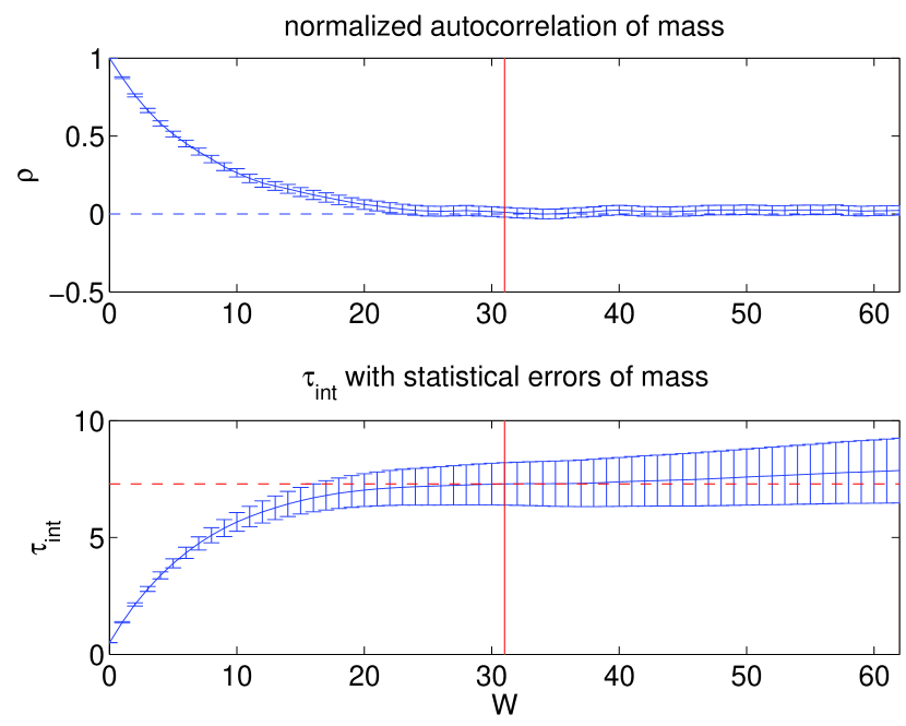
Figure 2: Generated plots of $\bar{\bar{\Gamma}}_{F}(t)$ and $\bar{\bar{\tau}}_{{\rm int},F}(W)$ with a vertical line at the $W$-value picked automatically and a horizontal one at the resulting estimate of $\tau_{{\rm int},F}$.

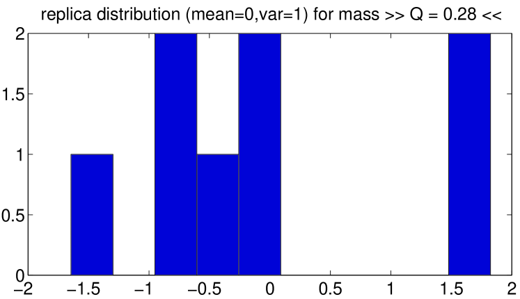
Figure 3: Replica distribution of $\{p_{r}\}$ with the $Q$-value in the title.

As a test case we think of determining the ‘effective’ mass

$$m=\ln(G(z)/G(z+1))=f(G(z),G(z+1))\equiv F$$ (67)

from a correlation $G(z)=\exp(-mz)$ in euclidean time $z$, which we take simply exponential since we are not interested here in systematic errors of $m$. To fake noisy (auto)correlated data for $G$ we employ normally distributed random numbers $\eta_{i},i=1,2,\ldots$ with zero mean and unit variance to produce a sequence $\{\nu_{i}\}$ by recursively setting

$$\nu_{1}=\eta_{1},\quad\nu_{i+1}=\sqrt{1-a^{2}}\,\eta_{i+1}+a\nu_{i},$$ (68)

with

$$\quad a=\frac{2\tau-1}{2\tau+1},\quad\tau\geq\frac{1}{2}.$$ (69)

A short calculation yields

$$\langle\,\nu_{i}\,\rangle=0,\quad\langle\,\nu_{i+t}\nu_{i}\,\rangle=a^{t},\quad\sum_{t=-\infty}^{\infty}a^{|t|}=2\tau.$$ (70)

We use three independent such sequences $\nu^{(1)}_{i},\nu^{(2)}_{i},\nu^{(3)}_{i}$ and choose for them integrated autocorrelation times $\tau^{(1)}<\tau^{(2)}=\tau^{(3)}$.

Synthetic data to measure $m=f(A_{1},A_{2})$ are formed,

$$a^{i}_{1}=G(0)+q(\nu^{(1)}_{i}+\nu^{(2)}_{i}),\quad a^{i}_{2}=G(1)+q(\nu^{(1)}_{i}+\nu^{(3)}_{i})\,.$$ (71)

The real parameter $q$ sets the strength of the noise, and the presence of $\nu^{(1)}_{i}$ in both observables creates a correlation between them, as in real life.

All relevant quantities of the error analysis can be worked out exactly for this case,

$$v_{A_{1}}=v_{A_{2}}=2q^{2},\quad\tau_{{\rm int},A_{1}}=\tau_{{\rm int},A_{2}}=(\tau^{(1)}+\tau^{(2)})/2,$$ (72)

$$v_{F}=2q^{2}(1+\exp(2m)-\exp(m)),$$ (73)

$$\tau_{{\rm int},F}=\frac{\hat{m}^{2}/2}{\hat{m}^{2}+1}\,\tau^{(1)}+\frac{\hat{m}^{2}/2+1}{\hat{m}^{2}+1}\,\tau^{(2)}$$ (74)

with

$$\hat{m}=2\sinh(m/2).$$ (75)

Note that in the weighed sum giving $\tau_{{\rm int},F}$ the time scale $\tau^{(1)}$ contributes with a small weight, due to correlations between $a_{i}^{1},a_{i}^{2}$ and the cancellation of the corresponding fluctuations in the effective mass.

For our test we now set $m=0.2,\tau^{(1)}=4,\tau^{(2)}=8,q=0.2$ which leads to $v_{F}=0.1016,\tau_{{\rm int},F}=7.92$. We generate $8\times 1000$ estimates corresponding to an error in the mass of 0.0142 and get

>> Nr=ones(8,1)*(N/8);
>> [value,dvalue,ddvalue,tauint,dtauint,Q]= ...
   UWerr(Data,1,Nr,’mass’,@effmass,1,2);
>> [value,dvalue,ddvalue,tauint,dtauint,Q]
ans =

    0.2128    0.0134    0.0008    7.2909    0.7396   0.2827

The generated plots are shown in Fig.2 and in Fig.3. By repeating such an analysis 20000 times we knock down the statistical error of the error far enough to exhibit a systematic error of $\sim-0.5\%$ which is of the expected order $\frac{1}{2}\exp(-W/\tau)$ with $W=37$ and $\tau=8$, while, of course, the actual automatic $W$ and estimated $\tau$-values fluctuate.

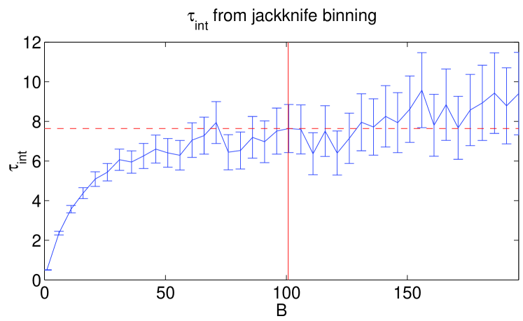
Figure 4: Estimation of $\tau_{{\rm int},F}$ by jackknife binning. A vertical line shows the optimal bin size (47).

The jackknife analog of the lower part of Fig.2 can be seen in Fig.4 for the same data. It looks consistent with a less pronounced plateau, as expected.

More relevant are tests on real data. The routine passed a number of such tests, but, as usual with software, with probability one some future application will force further evolution.

References

- [1] R. Frezzotti, M. Hasenbusch, U. Wolff, J. Heitger and K. Jansen, Comput. Phys. Commun. 136 (2001) 1, hep-lat/0009027.
- [2] U. Wolff, Monte Carlo error analysis, ALPHA collaboration, internal notes, 2002.
- [3] U. Wolff and B. Bunk, Lecture Notes on Computational Physics II [in german], www-com.physik.hu-berlin.de/comphys/comphys.html, Humboldt University, Berlin, 2002.
- [4] N. Madras and A.D. Sokal, J. Statist. Phys. 50 (1988) 109.
- [5] A.D. Sokal, Cours de Troisième Cycle, Lausanne, 1989.
- [6] W.H. Press, S.A. Teukolsky, W.T. Vetterling and B.P. Flannery, Numerical Recipes, Fortran, 2nd ed. (Cambridge University Press, 1992).
- [7] M. Lüscher, Comput. Phys. Commun. 165 (2005) 199, hep-lat/0409106.