Determination of the Improvement Coefficient ${c_{\rm SW}}$
up to One-Loop Order
with the Conventional Perturbation Theory

Abstract

We calculate the $O(a)$ improvement coefficient ${c_{\rm SW}}$ in the Sheikholeslami-Wohlert quark action for various improved gauge actions with six-link loops. We employ a conventional perturbation theory introducing the fictitious gluon mass to regularize the infrared divergence. Our results for some improved gauge actions are in agreement with those previously obtained with the Schrödinger functional method.

I Introduction

Recently the CP-PACS collaboration shows by a large scale of simulation that the hadron spectra in the quenched approximation systematically deviate from the experimentally observed ones both in the meson and the baryon sectorsquench . It is now obvious that the next step is to incorporate the effects of dynamical quarks to reproduce the correct hadron spectra. With the current computational resources, however, unquenched QCD simulations are often restricted on lattices with the lattice spacing coarser than 0.1 fm while keeping the physical volume larger than 2 fm.

A practical way to reduce the scaling violation effects is to employ the improved quark and gauge actions. For the quark part the $O(a)$ improved action proposed by Sheikholeslami and Wohlertsw is now widely used. This action requires only one new term called a clover term. Although from a theoretical point of view the plaquette gauge action is already $O(a)$ improved, a comparative numerical study employing the various quark and gauge actions shows that the renormalization group (RG) improved gauge action reduces non-negligible $O(a^{2})$ errorscompara . Moreover, JLQCD collaboration has recently reported that the first order phase transition observed in the three flavor QCD simulation with the $O(a)$ improved quark action and the plaquette gauge action, which is considered to be a lattice artifact, disappears once the gauge action is replaced by the RG improved onenf3 . Thus the improvement of the gauge action is mandatory for the three flavor QCD simulation at the currently accessible lattice spacing.

In this paper we determine the clover coefficient ${c_{\rm SW}}$ in the massless SW quark action up to one-loop order for various improved gauge actions including the DBW2 actiondbw2 . Preparing for new improved gauge actions yet to come, we parameterize the value of ${c_{\rm SW}}$ as a function of the improvement coefficient of gauge action for later convenience. Another important purpose of the present calculation is to check the validity of the conventional perturbative method for the determination of the massless clover coefficient ${c_{\rm SW}}$. Although previous calculations of ${c_{\rm SW}}$ are done by the twisted antiperiodic boundary conditionscsw_w or the Schrödinger functional methodcsw_sf , we instead employ the conventional perturbation theory with the use of the fictitious gluon mass to regularize the infrared divergence, which has been applied successfully for the calculation of the renormalization constants and the improvement coefficients for the bilinear quark operatorsgmass . This method can be easily implemented, within the standard knowledge of perturbation theory. Our results for some improved gauge actions are in agreement with those previously obtained with the Schrödinger functional method, which assures the validity of our conventional perturbative method. We are now extending this calculation of ${c_{\rm SW}}$ to the case of the heavy quark formulation proposed by the authorsakt , where the conventional perturbative method is much easier to handle the massive quarks than the Schrödinger functional method.

This paper is organized as follows. In Sec. II we introduce the improved quark and gauge actions and their Feynman rules relevant for the present calculation. In Sec. III we determine the clover coefficient ${c_{\rm SW}}$ up to one-loop level from the on-shell quark-quark scattering amplitude. The result of ${c_{\rm SW}}$ is parametrized as a function of the improvement coefficient of the gauge action. Our conclusions are summarized in Sec. IV.

The physical quantities are expressed in lattice units and the lattice spacing $a$ is suppressed unless necessary. We take SU($N_{c}$) gauge group with the gauge coupling constant $g$.

II Action and Feynman Rules

For the quark action we consider the $O(a)$-improved quark actionsw :

$$S_{\rm quark} = \sum_{n}\frac{1}{2}\sum_{\mu}\left\{{\bar{\psi}}_{n}(-r+\gamma_{\mu})U_{n,\mu}\psi_{n+{\hat{\mu}}}+{\bar{\psi}}_{n}(-r-\gamma_{\mu})U^{\dagger}_{n-{\hat{\mu}},\mu}\psi_{n-{\hat{\mu}}}\right\}+(m_{0}+4r)\sum_{n}{\bar{\psi}}_{n}\psi_{n}$$ (1)

$$-{c_{\rm SW}}\sum_{n}\sum_{\mu,\nu}ig\frac{r}{4}{\bar{\psi}}_{n}\sigma_{\mu\nu}F_{\mu\nu}(n)\psi_{n},$$

where we define the Euclidean gamma matrices in terms of the Minkowski matrices in the Bjorken-Drell convention: $\gamma_{j}=-i\gamma_{BD}^{j}$ $(j=1,2,3)$, $\gamma_{4}=\gamma_{BD}^{0}$, $\gamma_{5}=\gamma_{BD}^{5}$ and $\sigma_{\mu\nu}=\frac{1}{2}[\gamma_{\mu},\gamma_{\nu}]$. The field strength $F_{\mu\nu}$ in the clover term is given by

$$F_{\mu\nu}(n) = \frac{1}{4}\sum_{i=1}^{4}\frac{1}{2ig}\left(U_{i}(n)-U_{i}^{\dagger}(n)\right),$$ (2)

$$U_{1}(n) = U_{n,\mu}U_{n+{\hat{\mu}},\nu}U^{\dagger}_{n+{\hat{\nu}},\mu}U^{\dagger}_{n,\nu},$$ (3)

$$U_{2}(n) = U_{n,\nu}U^{\dagger}_{n-{\hat{\mu}}+{\hat{\nu}},\mu}U^{\dagger}_{n-{\hat{\mu}},\nu}U_{n-{\hat{\mu}},\mu},$$ (4)

$$U_{3}(n) = U^{\dagger}_{n-{\hat{\mu}},\mu}U^{\dagger}_{n-{\hat{\mu}}-{\hat{\nu}},\nu}U_{n-{\hat{\mu}}-{\hat{\nu}},\mu}U_{n-{\hat{\nu}},\nu},$$ (5)

$$U_{4}(n) = U^{\dagger}_{n-{\hat{\nu}},\nu}U_{n-{\hat{\nu}},\mu}U_{n+{\hat{\mu}}-{\hat{\nu}},\nu}U^{\dagger}_{n,\mu}.$$ (6)

The weak coupling perturbation theory is developed by writing the link variable in terms of the gauge potential

$$U_{n,\mu}=\exp\left(igaT^{A}A_{\mu}^{A}\left(n+\frac{1}{2}\hat{\mu}\right)\right),$$ (7)

where $T^{A}$ ($A=1,\dots,N^{2}_{c}-1$) is a generator of color SU($N_{c}$).

The quark propagator is obtained by inverting Wilson Dirac operator in eq.(1),

$$S_{q}^{-1}(p)=i\sum_{\mu}\gamma_{\mu}{\rm sin}(p_{\mu})+m_{0}+r\sum_{\mu}(1-{\rm cos}(p_{\mu})).$$ (8)

To calculate the improvement coefficient ${c_{\rm SW}}$ up to one-loop level, we need one-, two- and three-gluon vertices with quarks:

$$V^{A}_{1\mu}(p,q) = -gT^{A}\left\{i\gamma_{\mu}{\rm cos}\left(\frac{p_{\mu}+q_{\mu}}{2}\right)+r{\rm sin}\left(\frac{p_{\mu}+q_{\mu}}{2}\right)\right\},$$ (9)

$$V_{2\mu\nu}^{AB}(p,q) = \frac{a}{2}g^{2}\frac{1}{2}\{T^{A},T^{B}\}\delta_{\mu\nu}\left\{i\gamma_{\mu}\sin\left(\frac{p_{\mu}+q_{\mu}}{2}\right)-r\cos\left(\frac{p_{\mu}+q_{\mu}}{2}\right)\right\},$$ (10)

$$V_{3\mu\nu\tau}^{ABC}(p,q) = \frac{a^{2}}{6}g^{3}\frac{1}{6}\left[T^{A}\{T^{B},T^{C}\}+T^{B}\{T^{C},T^{A}\}+T^{C}\{T^{A},T^{B}\}\right]\delta_{\mu\nu}\delta_{\mu\tau}$$ (11)

$$\times\left\{i\gamma_{\mu}\cos\left(\frac{p_{\mu}+q_{\mu}}{2}\right)+r\sin\left(\frac{p_{\mu}+q_{\mu}}{2}\right)\right\},$$

$$V^{A}_{c1\mu}(p,q) = -gT^{A}{c_{\rm SW}}\frac{r}{2}\sum_{\nu}\sigma_{\mu\nu}\cos\left(\frac{p_{\mu}-q_{\mu}}{2}\right)\sin(p_{\nu}-q_{\nu}),$$ (12)

$$V^{AB}_{c2\mu\nu}(p,q,k_{1},k_{2}) = -\frac{a}{2}g^{2}if_{ABC}T^{C}{c_{\rm SW}}\frac{r}{4}$$

$$\times\left\{\sigma_{\mu\nu}\left[4\cos\left(\frac{k_{1\nu}}{2}\right)\cos\left(\frac{k_{2\mu}}{2}\right)\cos\left(\frac{q_{\mu}-p_{\mu}}{2}\right)\cos\left(\frac{q_{\nu}-p_{\nu}}{2}\right)\right.\right.$$

$$\left.\left.-2\cos\left(\frac{k_{1\mu}}{2}\right)\cos\left(\frac{k_{2\nu}}{2}\right)\right]\right.$$

$$\left.+\delta_{\mu\nu}\sum_{\rho}\sigma_{\mu\rho}\sin\left(\frac{q_{\mu}-p_{\mu}}{2}\right)\left[\sin(k_{2\rho})-\sin(k_{1\rho})\right]\right\},$$

$$V^{ABC}_{c3\mu\nu\tau}(p,q,k_{1},k_{2},k_{3}) = -3ig^{3}\frac{a^{2}}{6}{c_{\rm SW}}r$$

$$\times\left[T^{A}T^{B}T^{C}\delta_{\mu\nu}\delta_{\mu\tau}\sum_{\rho}i\sigma_{\mu\rho}\left\{-\frac{1}{6}\cos\left(\frac{q_{\mu}-p_{\mu}}{2}\right)\sin(q_{\rho}-p_{\rho})\right.\right.$$

$$\left.\left.+\cos\left(\frac{q_{\mu}-p_{\mu}}{2}\right)\cos\left(\frac{q_{\rho}-p_{\rho}}{2}\right)\cos\left(\frac{k_{3\rho}-k_{1\rho}}{2}\right)\sin\left(\frac{k_{2\rho}}{2}\right)\right\}\right.$$

$$\left.-\frac{1}{2}\left[T^{A}T^{B}T^{C}+T^{C}T^{B}T^{A}\right]i\sigma_{\mu\nu}\right.$$

$$\left.\times\left\{\delta_{\nu\tau}2\cos\left(\frac{q_{\mu}-p_{\mu}}{2}\right)\cos\left(\frac{q_{\nu}-p_{\nu}}{2}\right)\cos\left(\frac{k_{3\mu}+k_{2\mu}}{2}\right)\sin\left(\frac{k_{1\nu}}{2}\right)\right.\right.$$

$$\left.\left.+\delta_{\nu\tau}\sin\left(\frac{k_{3\nu}+k_{2\nu}}{2}\right)\cos\left(\frac{k_{1\mu}}{2}+k_{2\mu}\right)\right.\right.$$

$$\left.\left.+\delta_{\mu\tau}\sin\left(\frac{k_{1\mu}+2k_{2\mu}+k_{3\mu}}{2}\right)\cos\left(\frac{q_{\nu}-p_{\nu}}{2}\right)\cos\left(\frac{k_{3\nu}-k_{1\nu}}{2}\right)\right\}\right],$$

where $f_{ABC}$ the structure constant of SU($N_{c}$) gauge group. The first three vertices originate from the Wilson quark action and the last three from the clover term. The momentum assignments for the vertices are depicted in Fig. 1.

For the gauge action we consider the following general form including the standard plaquette term and six-link loop terms:

$$S_{\rm g}=\frac{1}{g^{2}}\left\{c_{0}\sum_{\rm plaquette}{\rm tr}U_{pl}+c_{1}\sum_{\rm rectangle}{\rm tr}U_{rtg}+c_{2}\sum_{\rm chair}{\rm tr}U_{chr}+c_{3}\sum_{\rm parallelogram}{\rm tr}U_{plg}\right\}$$ (15)

with the normalization condition

$$c_{0}+8c_{1}+16c_{2}+8c_{3}=1,$$ (16)

where six-link loops are composed of a $1\times 2$ rectangle, a bent $1\times 2$ rectangle (chair) and a three-dimensional parallelogram. In this paper we consider the following choices: $c_{1}=c_{2}=c_{3}=0$(Plaquette), $c_{1}=-1/12$, $c_{2}=c_{3}=0$(Symanzik)Weisz83 ; LW $c_{1}=-0.331$, $c_{2}=c_{3}=0$(Iwasaki), $c_{1}=-0.27,c_{2}+c_{3}=-0.04$(Iwasaki’) Iwasaki83 , $c_{1}=-0.252,c_{2}+c_{3}=-0.17$(Wilson)Wilson and $c_{1}=-1.40686$, $c_{2}=c_{3}=0$(DBW2)dbw2 . The last four cases are called the RG improved gauge action, whose parameters are chosen to be the values suggested by approximate renormalization group analyses. Some of these actions are now getting widely used, since they realize continuum-like gauge field fluctuations better than the naive plaquette action at the same lattice spacing.

The free gluon propagator is derived in Ref. Weisz83 :

$$D_{\mu\nu}(k) = \frac{1}{({\hat{k}}^{2})^{2}}\left[(1-A_{\mu\nu}){\hat{k}}_{\mu}{\hat{k}}_{\nu}+\delta_{\mu\nu}\sum_{\sigma}{\hat{k}}_{\sigma}^{2}A_{\nu\sigma}\right]$$ (17)

with

$${\hat{k}}_{\mu} = 2{\rm sin}\left(\frac{k_{\mu}}{2}\right),$$ (18)

$${\hat{k}}^{2} = \sum_{\mu=1}^{4}{\hat{k}}_{\mu}^{2},$$ (19)

where we employ the Feynman gauge. The matrix $A_{\mu\nu}$ satisfies

$$({\rm i}) A_{\mu\mu}=0\;\;\;{\rm for}\;\;{\rm all}\;\;\mu,$$ (20)

$$({\rm ii}) A_{\mu\nu}=A_{\nu\mu},$$ (21)

$$({\rm iii}) A_{\mu\nu}(k)=A_{\mu\nu}(-k).$$ (22)

$$({\rm iv}) A_{\mu\nu}(0)=1\;\;\;{\rm for}\;\;\mu\neq\nu,$$ (23)

and its expression is given by

$$A_{\mu\nu}(k) = \frac{1}{\Delta_{4}}\left[({\hat{k}}^{2}-{\hat{k}}_{\nu}^{2})(q_{\mu\rho}q_{\mu\tau}{\hat{k}}_{\mu}^{2}+q_{\mu\rho}q_{\rho\tau}{\hat{k}}_{\rho}^{2}+q_{\mu\tau}q_{\rho\tau}{\hat{k}}_{\tau}^{2})\right.$$ (24)

$$\left.+({\hat{k}}^{2}-{\hat{k}}_{\mu}^{2})(q_{\nu\rho}q_{\nu\tau}{\hat{k}}_{\nu}^{2}+q_{\nu\rho}q_{\rho\tau}{\hat{k}}_{\rho}^{2}+q_{\nu\tau}q_{\rho\tau}{\hat{k}}_{\tau}^{2})\right.$$

$$\left.+q_{\mu\rho}q_{\nu\tau}({\hat{k}}_{\mu}^{2}+{\hat{k}}_{\rho}^{2})({\hat{k}}_{\nu}^{2}+{\hat{k}}_{\tau}^{2})+q_{\mu\tau}q_{\nu\rho}({\hat{k}}_{\mu}^{2}+{\hat{k}}_{\tau}^{2})({\hat{k}}_{\nu}^{2}+{\hat{k}}_{\rho}^{2})\right.$$

$$\left.-q_{\mu\nu}q_{\rho\tau}({\hat{k}}_{\rho}^{2}+{\hat{k}}_{\tau}^{2})^{2}-(q_{\mu\rho}q_{\nu\rho}+q_{\mu\tau}q_{\nu\tau}){\hat{k}}_{\rho}^{2}{\hat{k}}_{\tau}^{2}\right.$$

$$\left.-q_{\mu\nu}(q_{\mu\rho}{\hat{k}}_{\mu}^{2}{\hat{k}}_{\tau}^{2}+q_{\mu\tau}{\hat{k}}_{\mu}^{2}{\hat{k}}_{\rho}^{2}+q_{\nu\rho}{\hat{k}}_{\nu}^{2}{\hat{k}}_{\tau}^{2}+q_{\nu\tau}{\hat{k}}_{\nu}^{2}{\hat{k}}_{\rho}^{2})\right],$$

with $\mu\neq\nu\neq\rho\neq\tau$ the Lorentz indices. $q_{\mu\nu}$ and $\Delta_{4}$ are written as

$$q_{\mu\nu} = (1-\delta_{\mu\nu})\left[1-(c_{1}-c_{2}-c_{3})({\hat{k}}_{\mu}^{2}+{\hat{k}}_{\nu}^{2})-(c_{2}+c_{3}){\hat{k}}^{2}\right],$$ (25)

$$\Delta_{4} = \sum_{\mu}{\hat{k}}_{\mu}^{4}\prod_{\nu\neq\mu}q_{\nu\mu}+\sum_{\mu>\nu,\rho>\tau,\{\rho,\tau\}\cap\{\mu,\nu\}=\emptyset}{\hat{k}}_{\mu}^{2}{\hat{k}}_{\nu}^{2}q_{\mu\nu}(q_{\mu\rho}q_{\nu\tau}+q_{\mu\tau}q_{\nu\rho}).$$ (26)

In the case of the standard plaquette action, the matrix $A_{\mu\nu}$ is simplified as

$$A_{\mu\nu}^{\rm plaquette}=1-\delta_{\mu\nu}.$$ (27)

The present calculation requires only the three-gluon vertex which is given in Ref. Weisz83 ,

$$V^{ABC}_{g3\lambda\rho\tau}(k_{1},k_{2},k_{3})=-i\frac{g}{6}f_{ABC}\sum_{i=0}^{3}c_{i}V^{(i)}_{g3\lambda\rho\tau}(k_{1},k_{2},k_{3})$$ (28)

with

$$V^{(0)}_{g3\lambda\rho\tau}(k_{1},k_{2},k_{3}) = \delta_{\lambda\rho}\widehat{(k_{1}-k_{2})}_{\tau}c_{3\lambda}+{\rm 2\;cycl.\;\;perms.},$$ (29)

$$V^{(1)}_{g3\lambda\rho\tau}(k_{1},k_{2},k_{3}) = 8V^{(0)}_{g3\lambda\rho\tau}(k_{1},k_{2},k_{3})$$ (30)

$$+\left[\delta_{\lambda\rho}\left\{c_{3\lambda}(\widehat{(k_{1}-k_{2})}_{\lambda}(\delta_{\lambda\tau}{\hat{k}}_{3}^{2}-{\hat{k}}_{3\lambda}{\hat{k}}_{3\tau})-\widehat{(k_{1}-k_{2})}_{\tau}({\hat{k}}_{1\tau}^{2}+{\hat{k}}_{2\tau}^{2}))\right.\right.$$

$$+ \left.\left.\widehat{(k_{1}-k_{2})}_{\tau}({\hat{k}}_{1\lambda}{\hat{k}}_{2\lambda}-2c_{1\lambda}c_{2\lambda}{\hat{k}}_{3\lambda}^{2})\right\}+{\rm 2\;cycl.\;\;perms.}\right],$$

$$V^{(2)}_{g3\lambda\rho\tau}(k_{1},k_{2},k_{3}) = 16V^{(0)}_{g3\lambda\rho\tau}(k_{1},k_{2},k_{3})$$ (31)

$$-\left[\delta_{\lambda\rho}(1-\delta_{\lambda\tau})c_{3\lambda}\sum_{\sigma\neq\lambda,\tau}\left\{\widehat{(k_{1}-k_{2})}_{\tau}({\hat{k}}_{1\sigma}^{2}+{\hat{k}}_{2\sigma}^{2}+{\hat{k}}_{3\sigma}^{2})+{\hat{k}}_{3\tau}({\hat{k}}_{1\sigma}^{2}-{\hat{k}}_{2\sigma}^{2})\right\}\right.$$

$$\left.+(1-\delta_{\lambda\rho})(1-\delta_{\lambda\tau})(1-\delta_{\rho\tau}){\hat{k}}_{1\lambda}{\hat{k}}_{2\rho}\widehat{(k_{1}-k_{2})}_{\tau}+{\rm 2\;cycl.\;\;perms.}\right],$$

$$V^{(3)}_{g3\lambda\rho\tau}(k_{1},k_{2},k_{3}) = 8V^{(0)}_{g3\lambda\rho\tau}(k_{1},k_{2},k_{3})$$ (32)

$$-\left[\delta_{\lambda\rho}(1-\delta_{\lambda\tau})c_{3\lambda}\widehat{(k_{1}-k_{2})}_{\tau}\sum_{\sigma\neq\lambda,\tau}({\hat{k}}_{1\sigma}^{2}+{\hat{k}}_{2\sigma}^{2})\right.$$

$$+\frac{1}{2}(1-\delta_{\lambda\rho})(1-\delta_{\lambda\tau})(1-\delta_{\rho\tau})\widehat{(k_{1}-k_{2})}_{\tau}\left\{{\hat{k}}_{1\lambda}{\hat{k}}_{2\rho}-\frac{1}{3}\widehat{(k_{3}-k_{1})}_{\rho}\widehat{(k_{2}-k_{3})}_{\lambda}\right\}$$

$$\left.+{\rm 2\;cycl.\;\;perms.}\right],$$

where we introduce the notation,

$$c_{i\lambda} = \cos\left(\frac{k_{i\lambda}}{2}\right).$$ (33)

The momentum assignment is found in Fig. 2.

III Determination of ${c_{\rm SW}}$ up to one-loop level

The first calculation of the clover coefficient up to the one-loop level ${c_{\rm SW}}={c_{\rm SW}}^{(0)}+g^{2}{c_{\rm SW}}^{(1)}$ was done by Wohlertcsw_w , who determined it for the plaquette gauge action to eliminate the $O(a)$ contribution in the on-shell quark-quark scattering amplitude. Since the gauge propagator is already $O(a)$ improved, the $O(a)$ contributions arise only from quark-gluon vertex. At tree-level the quark-gluon vertex in Fig. 3 is written as

$$\Lambda_{\mu}^{(0)}(p,q)=-gT^{A}\left\{i\gamma_{\mu}+r\left(\frac{p_{\mu}a+q_{\mu}a}{2}\right)\right\}-g\frac{r{c_{\rm SW}}}{2}T^{A}\sum_{\nu}\sigma_{\mu\nu}(p_{\nu}-q_{\nu})a+O(a^{2}).$$ (34)

where $p$ and $q$ are incoming and outgoing quark momenta assumed to be much less than the cutoff $a^{-1}$. We set the Wilson parameter to $r=1$. Sandwiching $\Lambda_{\mu}(p,q)$ by the Dirac spinor we obtain

$${\bar{u}}(q)\Lambda_{\mu}^{(0)}(p,q)u(p) = -gT^{A}{\bar{u}}(q)\{i\gamma_{\mu}+(1-{c_{\rm SW}}^{(0)})\frac{a}{2}(p_{\mu}+q_{\mu})\}u(p)+O(a^{2}),$$ (35)

where we use the Gordon identity. We find that ${c_{\rm SW}}^{(0)}$ should be one to eliminate the $O(a)$ term.

To determine the one-loop coefficient ${c_{\rm SW}}^{(1)}$ we need six types of diagrams shown in Fig. 4. The contribution of each diagram to the vertex function is denoted by

$$\Lambda_{\mu}^{(1)}(p,q)=\sum_{i=a,\dots,f}\Lambda_{\mu}^{(1-i)}(p,q)=\sum_{i=a,\dots,f}\int_{-\pi}^{\pi}\frac{d^{4}k}{(2\pi)^{4}}I_{\mu}^{(i)}(p,q,k).$$ (36)

Here we are concerned with the infrared divergences originating from some types of diagrams. Although they are supposed to be canceled out after summing up the contributions of all the diagrams, we need to introduce some infrared regularization in the process of the calculation. While previous calculations employ the twisted antiperiodic boundary conditionscsw_w or the Schrödinger functional methodcsw_sf for this purpose, we instead employ the fictitious gluon mass $\lambda$ with the ordinary perturbation theorygmass : the infrared divergences are extracted by an analytically integrable expression ${\tilde{I}}_{\mu}^{(i)}(p,q,k,\lambda)$ which has the same infrared behavior as $I_{\mu}^{(i)}(p,q,k)$,

$$\Lambda_{\mu}^{(1-i)}(p,q) = \int_{-\pi}^{\pi}\frac{d^{4}k}{(2\pi)^{4}}\theta(\Lambda^{2}-k^{2})\tilde{I}_{\mu}^{(i)}(p,q,k,\lambda)$$ (37)

$$+\int_{-\pi}^{\pi}\frac{d^{4}k}{(2\pi)^{4}}\left.\left\{I_{\mu}^{(i)}(p,q,k)-\theta(\Lambda^{2}-k^{2})\tilde{I}_{\mu}^{(i)}(p,q,k,\lambda)\right\}\right|_{\lambda\rightarrow 0}$$

with a cut-off $\Lambda$ $(\leq\pi)$. The Heaviside function $\theta$ is introduced to restrict the domain of integration to a hypersphere of radius $\Lambda$, which makes the integral analytically calculable. Since we are interested in the $O(g^{2}a)$ contributions, the counter terms ${\tilde{I}}_{\mu}^{(i)}(p,q,k,\lambda)$ can be composed of the propagators and vertices, obtained from an expansion of the Feynman rules in Sec. II up to $O(a)$:

$${\tilde{S}}_{q}(p) = \frac{-ip\kern-4.30554pt/+arp^{2}/2}{p^{2}},$$ (38)

$${\tilde{V}}^{A}_{1\mu}(p,q) = -gT^{A}\left\{i\gamma_{\mu}+\frac{a}{2}r(p_{\mu}+q_{\mu})\right\},$$ (39)

$${\tilde{V}}_{2\mu\nu}^{AB}(p,q) = \frac{a}{2}g^{2}\frac{1}{2}\{T^{A},T^{B}\}(-r)\delta_{\mu\nu},$$ (40)

$${\tilde{V}}^{A}_{c1\mu}(p,q) = -gT^{A}{c_{\rm SW}}\frac{ar}{2}\sum_{\nu}\sigma_{\mu\nu}(p_{\nu}-q_{\nu}),$$ (41)

$${\tilde{V}}^{AB}_{c2\mu\nu}(p,q,k_{1},k_{2}) = -\frac{a}{2}g^{2}if_{ABC}T^{C}{c_{\rm SW}}\frac{r}{2}\sigma_{\mu\nu},$$ (42)

$${\tilde{D}}_{\mu\nu}(k,\lambda) = \frac{\delta_{\mu\nu}}{k^{2}+\lambda^{2}},$$ (43)

$${\tilde{V}}^{ABC}_{g3\lambda\rho\tau}(k_{1},k_{2},k_{3}) = -i\frac{g}{6}f_{ABC}\left\{\delta_{\lambda\rho}(k_{1}-k_{2})_{\tau}+{\rm 2\;cycl.\;\;perms.}\right\},$$ (44)

where we consider the massless case. The momentum assignments are depicted in Figs. 1 and 2.

From the Lorentz symmetry and the parity conservation, the off-shell vertex function up to $O(p,q)$ is written as

$$\Lambda_{\mu}^{(1)}(p,q) = -g^{3}T^{A}\left\{\gamma_{\mu}F_{1}+aq\kern-4.30554pt/\gamma_{\mu}F_{2}+a\gamma_{\mu}p\kern-4.30554pt/F_{3}\right.$$ (45)

$$\left.+a(p_{\mu}+q_{\mu})G_{1}+a(p_{\mu}-q_{\mu})H_{1}+O(p^{2},q^{2},pq)\right\},$$

where $F_{i}$ $(i=1,2,3)$, $G_{1}$ and $H_{1}$ are dimensionless functions. Sandwiching $\Lambda_{\mu}^{(1)}(p,q)$ by the on-shell quark states the matrix elements are reduced to be

$${\bar{u}}(q)\Lambda_{\mu}^{(1)}(p,q)u(p) = -g^{3}T^{A}\left\{{\bar{u}}(q)\gamma_{\mu}u(p)F_{1}+a(p_{\mu}+q_{\mu}){\bar{u}}(q)u(p)G_{1}\right.$$ (46)

$$\left.+a(p_{\mu}-q_{\mu}){\bar{u}}(q)u(p)H_{1}\right\},$$

where $p\kern-4.30554pt/u(p)=0$ and ${\bar{u}}(q)q\kern-4.30554pt/=0$. From a view point of the on-shell improvement, the second and third terms of the right hand side represent the contributions of the dimension five operators,

$${\cal O}_{+} = (\partial_{\nu}\overline{\psi}(x))\sigma_{\mu\nu}\psi(x)+\overline{\psi}(x)\sigma_{\mu\nu}(\partial_{\nu}\overline{\psi}(x)),$$ (47)

$${\cal O}_{-} = (\partial_{\nu}\overline{\psi}(x))\sigma_{\mu\nu}\psi(x)-\overline{\psi}(x)\sigma_{\mu\nu}(\partial_{\nu}\overline{\psi}(x)).$$ (48)

Here we should note that the transformation property of ${\cal O}_{-}$ in terms of charge conjugation is different from that of $\overline{\psi}(x)\gamma_{\mu}\psi(x)$, which means that the last term of eq.(46) never appears, namely $H_{1}=0$. From the expression (45) we can extract the coefficient $G_{1}$ as

$$-g^{3}T^{A}G_{1} = \left.\frac{1}{8}{\rm Tr}\left[\left\{\frac{\partial}{\partial p_{\mu}}+\frac{\partial}{\partial q_{\mu}}\right\}\Lambda_{\mu}^{(1)}(p,q)+\left\{\frac{\partial}{\partial p_{\nu}}-\frac{\partial}{\partial q_{\nu}}\right\}\Lambda_{\mu}^{(1)}(p,q)\gamma_{\nu}\gamma_{\mu}\right]\right|^{\mu\neq\nu}_{p,q\rightarrow 0}$$ (49)

It would be instructive to show how the infrared divergence in each diagram cancels out after the summation. Let us take the case of the plaquette gauge action as an example. Including the constant terms we obtain

$$2G_{1}^{(a)} = -\frac{1}{N_{c}}(2{c_{\rm SW}}^{(0)}-1)L+0.004572(2),$$ (50)

$$2G_{1}^{(b)} = -\frac{N_{c}}{2}(6{c_{\rm SW}}^{(0)}-3)L+0.08311(3),$$ (51)

$$2G_{1}^{(c)} = \frac{N_{c}}{2}3{c_{\rm SW}}^{(0)}L-0.08133(3),$$ (52)

$$2G_{1}^{(d)} = 0.29739454(1),$$ (53)

$$2G_{1}^{(e)} = \frac{1}{2}\left\{-\left(C_{F}-\frac{1}{2N_{c}}\right)+\left(C_{F}+\frac{1}{2N_{c}}\right){c_{\rm SW}}^{(0)}\right\}L-0.017574(1),$$ (54)

$$2G_{1}^{(f)} = \frac{1}{2}\left\{-\left(C_{F}-\frac{1}{2N_{c}}\right)+\left(C_{F}+\frac{1}{2N_{c}}\right){c_{\rm SW}}^{(0)}\right\}L-0.017574(1),$$ (55)

where

$$L=\frac{1}{16\pi^{2}}\ln\left|\frac{\pi^{2}}{\lambda^{2}a^{2}}\right|$$ (56)

denotes the contribution of the infrared divergence with the fictitious gluon mass $\lambda$. The integrals are numerically estimated by a mode sum for a periodic box of a size $N^{4}$ with $N=64$ after transforming the momentum variable through $k^{\prime}_{\mu}=k_{\mu}-{\rm sin}k_{\mu}$. We choose $\Lambda=\pi$ for the cut-off. It is found that the tadpole diagram of Fig. 4 (d) gives the dominant contribution. The total contribution from infrared divergent terms becomes

$$L\times(1-{c_{\rm SW}}^{(0)})\left\{\frac{3}{2N_{c}}-C_{F}+\frac{3N_{c}}{2}\right\},$$ (57)

therefore, the infrared divergences are canceled out in a nontrivial way if and only if the tree-level coefficient is properly tuned: ${c_{\rm SW}}^{(0)}=1$. Whereas the coefficient of the logarithmic infrared divergence in each diagram is independent of the gauge action, the constant terms depend on it. In Table 1 we present the results of ${c_{\rm SW}}^{(1)}$ for the various improved gauge actions. The value of ${c_{\rm SW}}^{(1)}$ for DBW2 is obtained for the first time. Other results are consistent with those obtained by the previous work employing different infrared regularizationscsw_sf .

Here we give a brief description on the mean field improvement of ${c_{\rm SW}}$. The tadpole contribution of Fig. 4 is given by

$${c_{\rm SW}}^{\rm tad} = g^{2}{\int_{-\pi}^{\pi}\frac{d^{4}k}{(2\pi)^{4}}}\left[\left\{\left(\frac{4}{3}C_{F}+\frac{2}{3N_{c}}\right)-\left(\frac{3}{2N_{c}}-C_{F}\right)\sin^{2}\left(\frac{k_{\nu}}{2}\right)\right\}D_{\mu\mu}(k)\right.$$ (58)

$$\left.-\left(2C_{F}-\frac{1}{N_{c}}\right)\sin\left(\frac{k_{\mu}}{2}\right)\sin\left(\frac{k_{\nu}}{2}\right)D_{\mu\nu}(k)\right],$$

where $\mu$, $\nu$ are unsummed and $\mu\neq\nu$. The numerical values for the various gauge actions are listed in Table 1. The mean field improvement is applied as

$${c_{\rm SW}} = \left(1+\left(\frac{4}{3}C_{F}+\frac{2}{3N_{c}}\right)g^{2}T_{\rm MF}\right)\left(1+g^{2}{c_{\rm SW}}^{(1)}-\left(\frac{4}{3}C_{F}+\frac{2}{3N_{c}}\right)g^{2}T_{\rm MF}\right)+O(g^{4})$$ (59)

$$\rightarrow \frac{1}{u^{3}}\left(1+g^{2}{c_{\rm SW}}^{(1)}-\left(\frac{4}{3}C_{F}+\frac{2}{3N_{c}}\right)g^{2}T_{\rm MF}\right)+O(g^{4}),$$

where $u=P^{1/4}$ is evaluated by Monte Carlo simulation. The derivation of $T_{\rm MF}$ is given in detail in Sec. III of Ref. dwf_pt_rg .

The mean-field improved ${\overline{\rm MS}}$ coupling $g_{\overline{\rm MS}}^{2}(\mu)$ at the scale $\mu$ is obtained from the lattice bare coupling $g_{0}^{2}$ with the use of the following relation:

$$\displaystyle\frac{1}{g_{\overline{\rm MS}}^{2}(\mu)} = \displaystyle\frac{P}{g^{2}_{0}}+d_{g}+c_{p}+\displaystyle\frac{22}{16\pi^{2}}\log(\mu a)+N_{f}\left(d_{f}-\displaystyle\frac{4}{48\pi^{2}}\log(\mu a)\right).$$ (60)

For the improved gauge action one may use an alternative formulacppacs

$$\displaystyle\frac{1}{g_{\overline{\rm MS}}^{2}(\mu)} = \displaystyle\frac{c_{0}P+8c_{1}R1+16c_{2}R2+8c_{3}R3}{g^{2}_{0}}$$ (61)

$$+d_{g}+(c_{0}\cdot c_{p}+8c_{1}\cdot c_{R1}+16c_{2}\cdot c_{R2}+8c_{3}\cdot c_{R3})+\displaystyle\frac{22}{16\pi^{2}}\log(\mu a)$$

$$+N_{f}\left(d_{f}-\displaystyle\frac{4}{48\pi^{2}}\log(\mu a)\right),$$

where

$$P = \frac{1}{3}{\rm Tr}U_{plaquette}=1-c_{p}g_{0}^{2}+O(g_{0}^{4}),$$ (62)

$$R1 = \frac{1}{3}{\rm Tr}U_{rectangle}=1-c_{R1}g_{0}^{2}+O(g_{0}^{4}),$$ (63)

$$R2 = \frac{1}{3}{\rm Tr}U_{chair}=1-c_{R2}g_{0}^{2}+O(g_{0}^{4}),$$ (64)

$$R3 = \frac{1}{3}{\rm Tr}U_{parallelogram}=1-c_{R3}g_{0}^{2}+O(g_{0}^{4}),$$ (65)

and the measured values are employed for $P$, $R1$, $R2$ and $R3$. The values of $c_{p}$, $c_{R1}$, $c_{R2}$ and $c_{R3}$ for various gauge actions are listed in Table XVI of Ref. dwf_pt_rg .

For later convenience it would be a good idea to parameterize the value of ${c_{\rm SW}}^{(1)}$ as a function of $c_{1}$ while keeping $c_{2}=c_{3}=0$. In Fig. 5 we plot the results of ${c_{\rm SW}}^{(1)}$ evaluated by a mode sum with $N=64$, where $c_{1}$ is chosen from $-1.5$ to 0 at intervals of 0.02. We observe that ${c_{\rm SW}}^{(1)}$ seems to be divergent as $c_{1}$ increases. This behavior is well described by the rational expression,

$${c_{\rm SW}}^{(1)} = \frac{0.26849-0.14193c_{1}-0.13641c_{1}^{2}-0.07996c_{1}^{3}-0.01911c_{1}^{4}}{1-5.08365c_{1}}.$$ (66)

where the fitting result is also depicted in Fig. 5. The difference between the actual value and the fit is less than 0.1% for $-1.5\leq c_{1}\leq 0$.

IV Conclusion

In this paper we determine the clover coefficient ${c_{\rm SW}}$ in the massless SW quark action up to one-loop order for the various improved gauge actions employing the conventional perturbative method with the fictitious gluon mass as an infrared regulator. The validity of the method is checked by comparing the results to those previously obtained by the Schrödinger functional method: both show a good agreement within error bars. For later convenience our results are parametrized in terms of the improvement coefficient $c_{1}$ of the gauge action. An important application of this conventional perturbative method is to determine ${c_{\rm SW}}$ for the massive quarks in the heavy quark formulation proposed by the authors, where the relativistic on-shell improvement is extended to the massive case including any power corrections of $m_{Q}a$. Whereas $c_{E}$ and $c_{B}$ receive different $m_{Q}a$ corrections in this formulation, a modification of the present calculational techniques can be done in a straightforward mannercsw_m .

Table 1: One-loop coefficient of ${c_{\rm SW}}$ for various improved gauge actions. Tadpole contribution of Fig. 4 (d) is also listed.

gauge action	$c_{1}$	$c_{3}$	${c_{\rm SW}}^{(1)}$	${c_{\rm SW}}^{\rm tad}$
plaquette	0	0	0.26858825(1)	0.29739454(1)
Symanzik	–1/12	0	0.19624449(1)	0.23543879(1)
Iwasaki	–0.331	0	0.11300591(1)	0.15988461(1)
Iwasaki’	–0.27	–0.04	0.12036501(1)	0.16566349(1)
Wilson	–0.252	–0.17	0.10983411(1)	0.15292225(1)
DBW2	–1.40686	0	0.04243181(1)	0.08997537(1)

Figure 1: Momentum assignments for the quark-gluon vertices.

Figure 2: Momentum assignment for the three-gluon vertex.

Figure 3: Quark-gluon vertex at tree level.

Figure 4: Quark-gluon vertex at one-loop level.

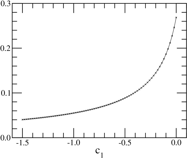
Figure 5: ${c_{\rm SW}}^{(1)}$ as a function of $c_{1}$ with $c_{2}=c_{3}=0$. Solid line denotes the fitting result of eq.(66).

References

• (1) CP-PACS Collaboration (S.Β Aoki et al.), Phys.Β Rev.Β Lett.Β 84 (2000) 238; Phys.Β Rev.Β D67 (2003) 034503.
• (2) B.Β Sheikholeslami and R.Β Wohlert, Nucl. Phys. B259 (1985) 572.
• (3) CP-PACS Collaboration (S. Aoki et al.), Phys.Β Rev.Β D60 (1999) 114508.
• (4) JLQCD Collaboration (S.Β Aoki et al.), Nucl.Β Phys.Β Proc.Β Suppl.Β 106 (2002) 263.
• (5) T.Β Takaishi, Phys.Β Rev. D54 (1996) 1050; P.Β deΒ Forcrand et al., Nucl.Β Phys. B577 (2000) 263.
• (6) R.Β Wohlert, DESY preprint 87-069 (1987), unpublished.
• (7) M.Β LΓΌscher and P.Β Weisz, Nucl. Phys. B479 (1996) 429; S.Β Aoki, R.Β Frezzotti and P.Β Weisz, Nucl. Phys. B540 (1999) 501.
• (8) S.Β Aoki, K.Β Nagai, Y.Β Taniguchi and A.Β Ukawa, Phys. Rev. D58 (1998) 074505; Y.Β Taniguchi and A.Β Ukawa, Phys. Rev. D58 (1998) 114503.
• (9) S.Β Aoki, Y.Β Kuramashi and S.Β Tominaga, Prog.Β Theor.Β Phys.Β 109 (2003) 383.
• (10) P.Β Weisz, Nucl.Β Phys. B212 (1983) 1; P.Β Weisz and R.Β Wohlert, Nucl.Β Phys. B236 (1984) 397; erratum, ibid. B247 (1984) 544.
• (11) M.Β LΓΌscher and P.Β Weisz, Commun.Β Math.Β Phys. 97 (1985) 59; erratum, ibid. 98 (1985) 433.
• (12) Y.Β Iwasaki, preprint, UTHEP-118 (Dec. 1983), unpublished.
• (13) K.Β G.Β Wilson, in Recent Development of Gauge Theories, eds. G. ’tHooft et al. (Plenum, New York, 1980).
• (14) S.Β Aoki, T.Β Izubuchi, Y.Β Kuramashi and Y.Β Taniguchi, Phys.Β Rev.Β D67 (2003) 094502.
• (15) A.Β Ali Khan et al., Phys. Rev. D65 (2002) 054505; erratum, ibid.Β D67 (2003) 059901.
• (16) S.Β Aoki, Y.Β Kayaba and Y.Β Kuramashi, in preparation.